Stochastic Growth Models for the Spreading of Fake News

Abstract

The propagation of fake news in online social networks nowadays is becoming a critical issue. Consequently, many mathematical models have been proposed to mimic the related time evolution. In this work, we first consider a deterministic model that describes rumor propagation and can be viewed as an extended logistic model. In particular, we analyze the main features of the growth curve, such as the limit behavior, the inflection point, and the threshold-crossing-time, through fixed boundaries. Then, in order to study the stochastic counterparts of the model, we consider two different stochastic processes: a time non-homogeneous linear pure birth process and a lognormal diffusion process. The conditions under which the means of the processes are identical to the deterministic curve are discussed. The first-passage-time problem is also investigated both for the birth process and the lognormal diffusion process. Finally, in order to study the variability of the stochastic processes introduced so far, we perform a comparison between their variances.

1. Introduction

Several types of real growth dynamics can be described by mathematical models. The most simple model is the Malthusian one in which the population size grows in time as an exponential function. Clearly, this model, in some instances, turns out not to be fully appropriate since it possesses an infinite limit value. Indeed, for long-term growth, it is necessary to take into account factors which can slow down or speed up the growth rate of the population. Aiming to describe these real situations, one can refer to so-called sigmoidal growth models, characterized by an initial slow growth followed by an explosion of an exponential-type, which finally flattens out to an equilibrium status, known as the carrying capacity.

Over the years, several sigmoidal curves have been introduced, such as Gompertz (see Tan [1]), Korf (introduced for the first time in Korf [2]), logistic (see, for instance, Di Crescenzo and Paraggio [3]), Bertalanffy–Richards (Richards [4]), and other generalizations of already existing models (as in Asadi et al. [5], Di Crescenzo and Spina [6], Di Crescenzo et al. [7,8]). The fields of possible applications of sigmoidal models are various and range from software reliability (see Erto et al. [9]) to biology (as in Brauer and Castillo-Chavez [10]) and economics (see, for example, Smirnov and Wang [11]).

Recently, S-shaped models have been used to model the spread of rumors in online social networks (see San Martìn et al. [12]). The attention stimulated by this topic arises from the global increase in social network usage and the ease of sending messages instantaneously. The growth of instantaneous communication has proved to be a fertile ground for the spread of fake news (see De Martino and Spina [13], Giorno and Spina [14], Figueira and Oliveira [15]).

By the term ‘fake news’, we generally mean false or misleading information. The techniques used to generate fake news have been the subject of many investigations, such as research reports by the RAND Corporation. Accordingly, in a broad sense, fake news can be characterized as follows:

(i)

Fabrication: the invention of entirely false or misleading information,

(ii)

Misappropriation: the misrepresentation of existing facts, events and people,

(iii)

Deceptive identities: the employment of misleading source of information,

(iv)

Obfuscation: the offering of multiple and contradictory accounts for the same event in order to confuse the audience,

(v)

Conspiracy theories: the proposal of conspiracy plots related to real events/phenomena,

(vi)

Selective use of facts: the selection of information in a manipulative way,

(vii)

Rhetorical fallacies: reasoning which is logically invalid but cognitively effective,

(viii)

Appeals to emotion/authority: the use of messages which elicit emotions.

The diffusion of fake news, whether intentional or accidental, causes disinformation which may be used for various aims, such as influencing public opinion, instigating hatred, damaging the image of particular states/companies, etc. Hence, studying the propagation of rumors and disinformation may be of great interest in order to design countermeasures and avoid potential impacts on society. The urgency of the matter has prompted various states, and also private companies, to invest in cybersecurity. In this context, a great deal of scientific research effort has been invested, especially in relation to the proposal of stochastic models with effective predictive capabilities (see, for instance, Abraham and Nair [16], Abimbola et al. [17], Paul and Zhang [18], Alandihallaj et al. [19]). In addition, the further need to optimize investments in cybersecurity also arises. This topic has been addressed in the work of Miaoui and Boudriga [20]. In particular, these authors propose a model that optimizes enterprise investments in cybersecurity using expected utility theory.

The development of suitable mathematical models capable of simulating the propagation of rumors is potentially of considerable value in making strategic choices (see, for example, Mahmoud [21], Kapsikar et al. [22], Ben Aissa et al. [23]). However, the development of stochastic models relating to the spread of information is not an easy task. Indeed, as noted in Raponi et al. [24], the propagation of fake news is a complex phenomenon influenced by several factors the identification and assessment of which is challenging. To overcome this difficulty, many models have been proposed in the literature that have been inspired by epidemiological models. However, although the two contexts have various similarities, the dissemination of news follows different rules than the diffusion of contagious diseases. Thus, a variety of models in stochastic environments has been developed which emphasize different aspects of interest. For instance, Esmaeeli and Sajadi [25] developed a sceptical rumor model for individuals located on a non-negative integer line, whereas a case illustrating the spread of fake news in a community of finite size was considered by Mahmoud [21]. Moreover, recent developments in stochastic rumor propagation modeling can be found in Jia and Cao [26] and Roy and Saha [27].

Nevertheless, although many attempts have been made, a model that includes all the properties of the real fake-news propagation phenomenon has not yet been reported. Bearing in mind the complexity of the problems connected to the phenomenon, the aim of this paper is twofold: (i) to study and enhance a recent growth model for rumor propagation, (ii) to build and study two stochastic processes that are able to describe the growth model itself in the presence of random fluctuations. In contrast to stochastic models treated in [21,25,26,27], which are based on spatial dynamics on suitable state-spaces and depend on network topologies, for analysis of point (ii), we focus on time-inhomogeneous settings involving suitable birth–death and diffusion processes whose means are identical to the growth model considered in point (i).

Usually, growth models are described by means of differential equations. In order to make them more realistic, it is possible to introduce a noise term, summarizing random fluctuations, in the differential equations (see Øksendal [28]) and to consider the resulting stochastic differential equations (as reported in Román-Román et al. [29] and Di Crescenzo et al. [7]). Other investigations have proposed introducing a random environment by considering special birth–death processes using an expected value which corresponds to the deterministic growth function (see Di Crescenzo and Spina [6], Di Crescenzo and Paraggio [3], Giorno and Nobile [30], Ricciardi [31]).

Hence, in the present work, we analyze both of the strategies stimulated by the above mentioned research lines.

A key concern with regard to disinformation and fake news that has recently emerged is the need for reassurance on the validity and quality of the news in the face of new pitfalls that can arise by use of the Web and from the use of artificial intelligence (AI). Major efforts are, therefore, needed to create a stable alliance between all stakeholders to promote, by any means, communication and awareness-raising activities aimed at all users so that they are able to recognize bad information and protect themselves from the dangers that can arise from it. Therefore, tools pertaining to AI can be fruitfully used to support the collective efforts of relevant institutions, web companies and communication professionals which are called upon to implement clear and shared actions to counter disinformation and the spread of fake news. Hence, identifying and extracting the most appropriate and significant features from information flows is one of the biggest challenges for AI-based detection. In this area, examples of recent contributions related to feature extraction and anomaly detection can be found in Khan et al. [32] and Arunnehru et al. [33].

We focus on the growth model proposed by San Martin et al. [12] for rumor propagation, postponing consideration of AI-based strategies for future work.

In this paper, our investigation is described along the following novel lines:

(i)

analyzing some limit behaviors of the growth function, which is shown to be a suitable extension of the logistic curve,

(ii)

studying the corresponding mean time in which a randomly chosen individual is reached by the rumor,

(iii)

determining the initial specific growth rate, the inflection point, and other related quantities,

(iv)

conducting a sensitivity analysis based on the perturbation on the parameters of the model,

(v)

addressing the related threshold-crossing problem,

(vi)

studying and comparing two different stochastic counterparts for the model based on suitable time-inhomogenous Markov processes, i.e., a linear birth–death process and a lognormal diffusion process.

Specifically, we provide conditions such that the mean values of these stochastic processes are identical to the growth curve, which allows modeling of the diffusion of rumors in the presence of random fluctuations. Moreover, we provide explicit expressions for various quantities of interest in applications, such as the conditional mean, the conditional variance, the index of dispersion, and the Fano factor. Finally, in order to investigate the variability of the two considered stochastic processes, we perform a comparison of their variances.

1.1. Relation with Epidemiological Models

Usually, propagation models for rumors are very similar to those used for the spread of infectious diseases. One of the best-known epidemiological models is the SI model, according to which the population is divided into two categories, i.e., susceptible and infected. In this case, the resulting growth curve describing the time evolution of those infected follows an exponential trend. In other recent studies, various generalizations of compartmental models have been introduced. For example, in Jin et al. [34] the authors consider the population to be divided into susceptible, exposed, infected (i.e., reached by the rumor) and skeptics (SEIZ model). Similarly, in [14] the population is divided into three classes: ignorant, spreader and stifler. In all the aforementioned studies, the model which mimics the dynamics of rumor spread is represented by a system of differential equations (one equation for any compartment). In other studies, researchers have focused on analysis of the time evolution of a rumor among the population by considering only one of the compartments into which the population is divided. This is the case as reported in [13], where the authors consider a differential equation describing the time evolution of infected individuals. In particular, the considered differential equation is a logistic one with a time-dependent growth rate. In the present paper, we consider an existing model which represents the fraction of the population reached by the rumor. This growth model embodies both the exponential and the logistic one. Indeed, they can be recovered by considering the special limit values of the parameters (cf. Section 2 below). Clearly, to have a more realistic representation of the rumor spread among individuals in a population, it may be interesting to consider a suitable compartmental model and its stochastic counterpart. This topic may be the subject of future investigations.

1.2. Plan of the Paper

The paper is organized in detail as follows: In Section 2, we study the main features of the deterministic model introduced in [12], such as the carrying capacity and the inflection point. A sensitivity analysis based on perturbation of the parameters and a study related to the problem of the first-crossing-time of the special threshold are also performed. Moreover, we analyze the expected time in which a randomly chosen individual is reached by the rumor. Then, in Section 3, we define a special time-inhomogeneous linear pure birth process having a mean which corresponds to the deterministic curve of Section 2. For this process, the transition probabilities, the moment-generating function, the variance, and some indexes of dispersion, are also determined. The first-passage-time problem of the pure birth process through constant boundaries is also addressed. Section 4 is devoted to description of a special lognormal diffusion process having the same mean as the pure birth process introduced in Section 3. The moments, the mode, and the quantiles of this process are also provided in closed form. Moreover, we study the first-passage-time problem by considering particular time-dependent boundaries in order to obtain an explicit expression for the corresponding probability density function. Finally, in order to provide a comparison between the stochastic processes introduced previously, since they possess the same mean, we investigate the ratio between their variances.

2. The Deterministic Model

In San Martín et al. [12], the authors propose a novel mathematical model to represent the spread of rumors in online social networks. It is assumed that the individuals are linked either by person-to-person relations or by belonging to the same group. Moreover, in the considered model, the population is divided into four categories: burned, sender, receiver and seed.

(i)

A burned individual is defined as a person who knows the rumor. Note that when an individual becomes burned, he/she remains in this state until the end of rumor propagation.

(ii)

A sender is a person who knows the message and texts it to his/her contacts.

(iii)

A receiver is an individual who is reached by the rumor.

(iv)

Finally, the seed is the set of all the individuals who know the rumor at the beginning of its propagation.

Note that the aforementioned categories are not mutually disjoint. For example, a sender is also a burned individual and a receiver may be also be an already burned individual.

In this work, we focus our attention on the function $F\left(t\right)$ that represents the fraction of burned individuals at the time $t\ge 0$. According to Equation (3) of [12] with $a=1$ and $b=0$, it is defined as follows

$$F\left(t\right)=\frac{Cexp\left((1+\epsilon )t\right)-1}{Cexp\left((1+\epsilon )t\right)+\frac{2\epsilon }{1-\epsilon }},t\ge 0,$$

(1)

where $C\ge 1$ and $-1<\epsilon <1$. The positions performed in Equation (3) of [12] correspond to consider the original time scale ($a=1$) and take 0 as the time origin ($b=0$). According to the assumption specified in (i), from Equation (1), we have that the function $F\left(t\right)$ is monotone non-decreasing in $t\ge 0$, and satisfies $0\le F\left(t\right)\le 1$ for all $t\ge 0$.

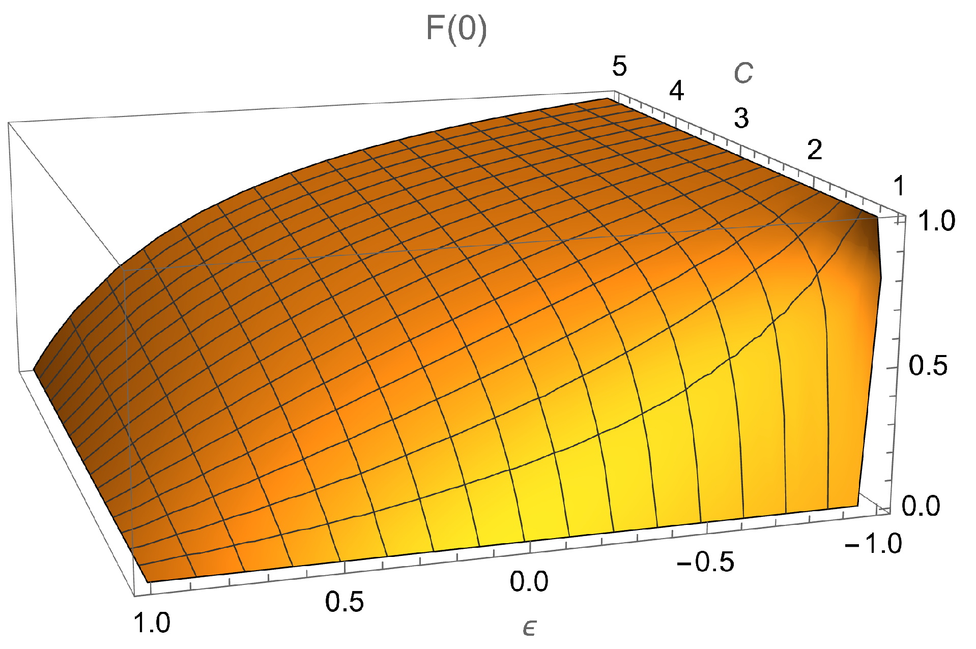
Remark 1.

From Equation (1), we have that the carrying capacity of the population, obtained as ${lim}_{t\to \infty }F\left(t\right)$, is equal to 1. In other terms, the percentage of the population that will eventually be informed about the rumor is unity.

Moreover, $F\left(t\right)$ is the solution of the following differential equation

$$\frac{\mathrm{d}}{\mathrm{d}t}F\left(t\right)=2\epsilon \left(\frac{1-\epsilon }{2\epsilon }+F\left(t\right)\right)(1-F\left(t\right)),t\ge 0,$$

(2)

with the initial condition due to Equation (1) for $t=0$, i.e.,

$$F\left(0\right)=\frac{C-1}{C+\frac{2\epsilon }{1-\epsilon }}\ge 0.$$

(3)

From the above formulas, we have that the parameter $\epsilon$ is involved both in the differential Equation (2) and the initial condition (3), whereas the parameter C is only linked to the initial size of the burned individuals $F\left(0\right)$. Clearly, a large value of C, or $\epsilon$ close to $-1$, correspond to a large initial size of burned individuals. Figure 1 illustrates the behavior of $F\left(0\right)$, which is decreasing in $\epsilon$ and increasing in C.

The parameters $\epsilon \in (-1,1)$ and $C\ge 1$ allow obtaining different kinds of growth, including the limit cases $\epsilon \to -1$ and $\epsilon \to 1$. Let us now examine some features.

• Case no. 1:  $\epsilon \to -1$

If $\epsilon \to -1$, then Equations (2) and (3) yield the differential problem

$$\left\{\begin{array}{c}{\displaystyle \frac{\mathrm{d}}{\mathrm{d}t}F\left(t\right)=2{(1-F\left(t\right))}^2,t\ge 0,}\hfill \\ F\left(0\right)=1\hfill \end{array}\right.$$

with trivial constant solution

$$F\left(t\right)=1,t\ge 0.$$

In this case, all the individuals already know the rumor since the beginning.

• Case no. 2:  $\epsilon \to 0$

When $\epsilon \to 0$, from (2) and (3), we have

$$\left\{\begin{array}{c}{\displaystyle \frac{\mathrm{d}}{\mathrm{d}t}F\left(t\right)=1-F\left(t\right),t\ge 0,}\hfill \\ F\left(0\right)=\frac{C-1}{C}\hfill \end{array}\right.$$

so that

$$F\left(t\right)=1-\frac{1}{C}{e}^{-t},t\ge 0.$$

(4)

In this case, the spread of the rumor among the individuals grows in an (increasingly concave) exponential way.

• Case no. 3:  $\epsilon \to 1$

If $\epsilon \to 1$, then Equations (2) and (3) give the problem

$$\left\{\begin{array}{c}{\displaystyle \frac{\mathrm{d}}{\mathrm{d}t}F\left(t\right)=2(1-F\left(t\right))F\left(t\right),t\ge 0,}\hfill \\ F\left(0\right)=0\hfill \end{array}\right.$$

which corresponds to the logistic model starting with a vanishing initial solution (for instance, cf. Remark 2.1 of Albano et al. [35]). In this case, the solution is trivially

$$F\left(t\right)=0,t\ge 0,$$

so that, if no individuals know the rumor at the beginning, then it does not spread in the population.

• Case no. 4:  $C=1$

If $C=1$ then $F\left(0\right)=0$, so that no individuals know the rumor at the beginning. However, in this case, Equation (1) is still a non-trivial function of t. Indeed, for $\epsilon \in (-1,1)$, the rumor can spread among the population, whereas when $\epsilon \to 1$, the rumor cannot spread anymore. Moreover, for $C=1$, from Equations (2) and (3), we have $\frac{d}{dt}F\left(t\right){|}_{t=0}=1-\epsilon$, so that, in this case, $\epsilon$ can be viewed as a reversed measure of the initial intensity of rumor spreading.

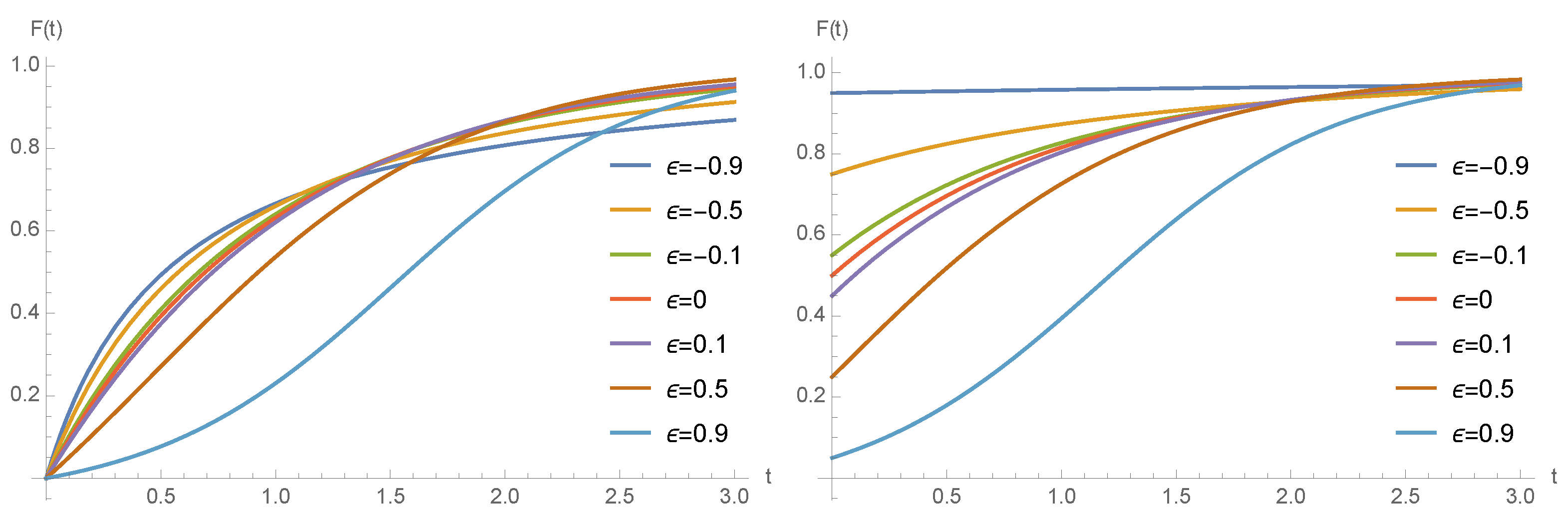
In Figure 2, some plots of the function $F\left(t\right)$ are provided for different choices of both the parameters C and $\epsilon$. The first frame, for $C=1$, confirms the remarks stated in Case no. 4, in particular that the initial intensity of rumor spreading is decreasing for $\epsilon \in (-1,1)$. This behavior is exhibited also for $C=2$, as shown in in the second frame of Figure 2, where it is also evident that $F\left(0\right)$ is decreasing in $\epsilon$ due to (3).

Concerning the complexity of the model, it is not hard to see that the function (1) is $O\left(g\right(t\left)\right)$, where $g\left(t\right)=1-\frac{1}{C}{e}^{-t}$, $t\ge 0$, corresponds to the growth function obtained in Equation (4) in the limit as $\epsilon \to 0$.

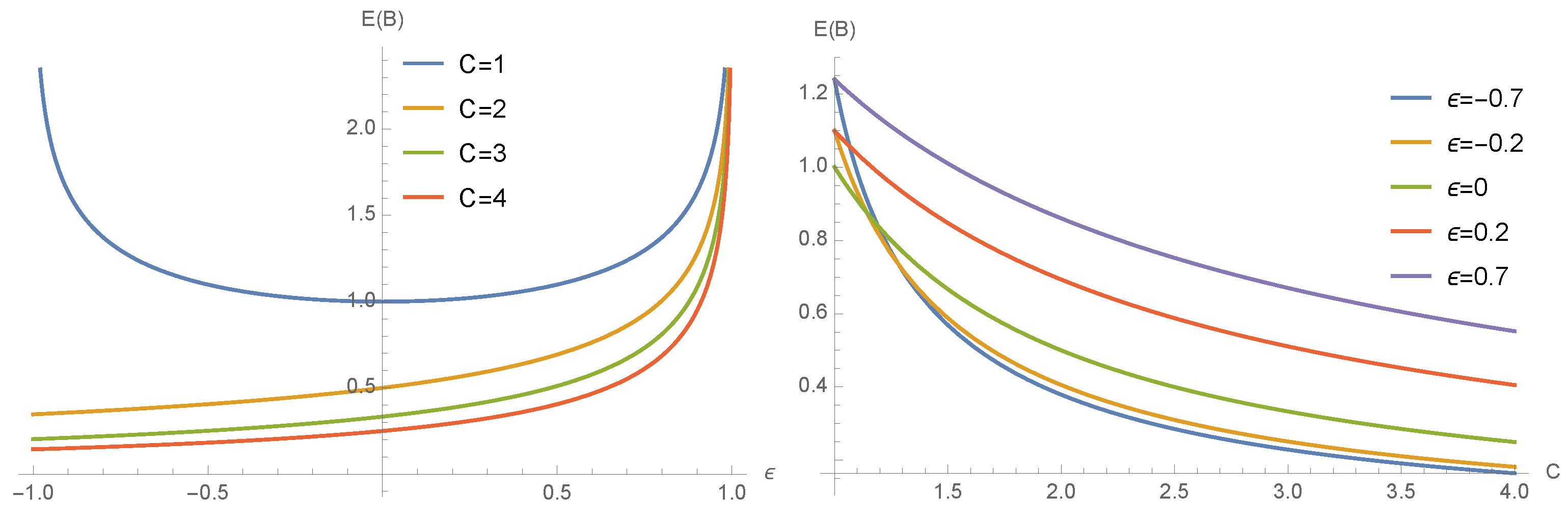
Remark 2.

It is worth noting that $F\left(t\right)$ may be viewed as the distribution function of a random variable, say B, having support $[0,+\infty )$, which describes the instant in which an individual randomly chosen in the population is reached by the rumor. Clearly, due to (1) and (3), one has that B is absolutely continuous if, and only if, $C=1$, whereas for $C>1$, it is a mixed random variable, with an atom at 0 (corresponding to the individuals informed at time 0). The corresponding mean $\mathsf{E}\left(B\right)$ represents the expected time in which a randomly chosen individual is reached by the rumor, with

$$\begin{array}{cc}\hfill \mathsf{E}\left(B\right)& ={\int }_0^{+\infty }\mathsf{P}(B>t)\mathrm{d}t={\int }_0^{+\infty }\left[1-F\left(t\right)\right]\mathrm{d}t\hfill \\ \hfill & =\left\{\begin{array}{cc}{\displaystyle \frac{1}{2\epsilon }log\left(1+\frac{2\epsilon }{C(1-\epsilon )}\right),}\hfill & \mathit{if}\epsilon \in (-1,0)\cup (0,1),\hfill \\ {\displaystyle \frac{1}{C},}\hfill & \mathit{if}\epsilon =0.\hfill \end{array}\right.\hfill \end{array}$$

Note that $\mathsf{E}\left(B\right)$ is decreasing with respect to C; moreover, for $C=1$, it is an even convex function in ε. These comments are confirmed by Figure 3, which shows some plots of $\mathsf{E}\left(B\right)$.

2.1. A Different Formulation

It has been pointed out in various recent investigations on population dynamics that problems concerning differential equations of the form (2) can, in some instances, be expressed in a different way (cf. [3,6,7,8]). In this vein, the present section is devoted to the determination of a different formulation of Equation (2), introducing a time-dependent growth rate. In more detail, in our case, the function (1) can also be viewed as a solution of the following differential equation

$$\frac{\mathrm{d}}{\mathrm{d}t}F\left(t\right)=\xi \left(t\right)F\left(t\right),t\ge 0,$$

(5)

where the time-dependent growth rate $\xi \left(t\right)$ has the following expression

$$\xi \left(t\right)=\frac{C{e}^{(1+\epsilon )t}{(1+\epsilon )}^2}{(C{e}^{(1+\epsilon )t}-1)(2\epsilon +(1-\epsilon )C{e}^{(1+\epsilon )t})},t\ge 0.$$

(6)

We note that the growth rate (6) is decreasing in $t\ge 0$; this implies that the intensity of information spread gradually fades over time. Clearly, since the differential Equation (5) is a reformulation of the same problem described by Equations (2) and (3), the solution $F\left(t\right)$ is still expressed by (1).

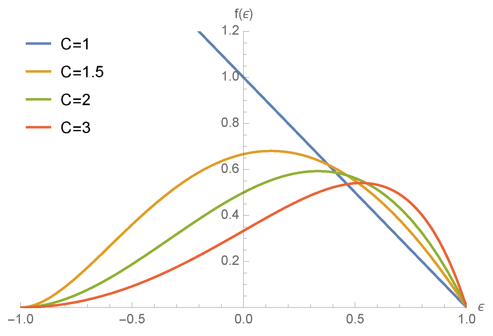
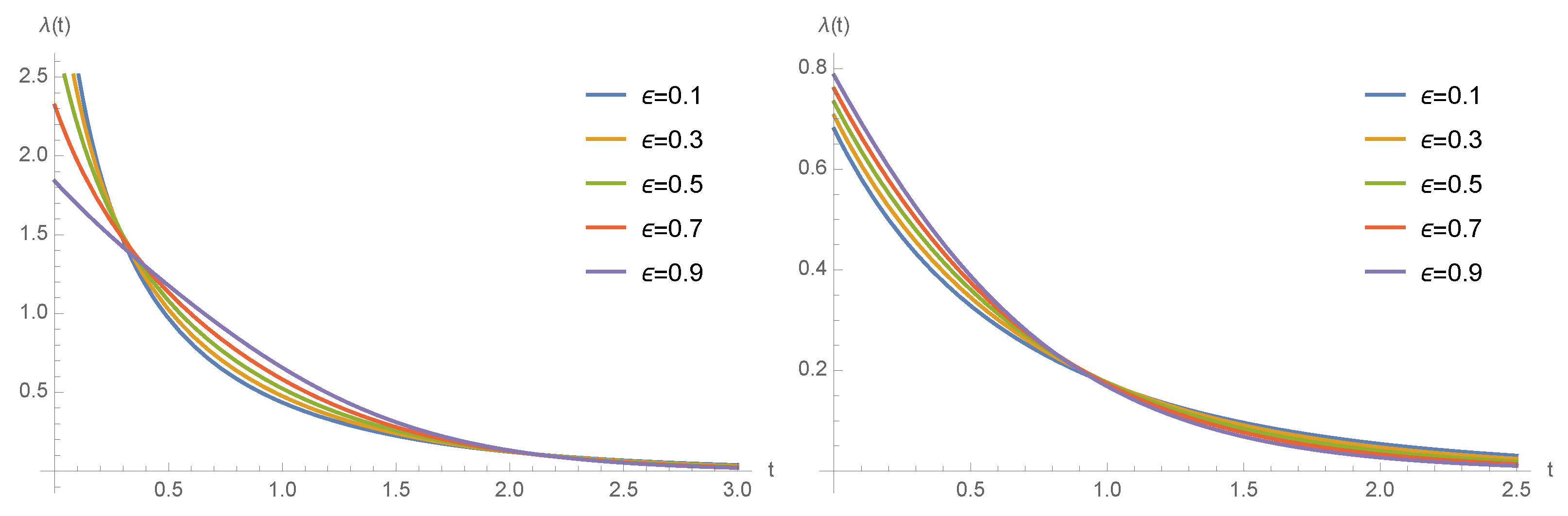
Let us now introduce the function

$$f\left(\epsilon \right):=\frac{C(1-\epsilon ){(1+\epsilon )}^2}{{(C+2\epsilon -C\epsilon )}^2}\equiv \frac{\mathrm{d}}{\mathrm{d}t}F\left(t\right){|}_{t=0}=\xi \left(0\right)F\left(0\right).$$

(7)

This function can be viewed as the initial specific growth rate, since it describes the slope of the tangent to che curve $F\left(t\right)$ for $t=0$. With respect to its behavior as a function of $\epsilon \in (-1,1)$, from (7), we have two cases:

(a)

if $C=1$, and, thus, $F\left(0\right)=0$, then, $f\left(\epsilon \right)$ is linearly decreasing, being $f\left(\epsilon \right)=1-\epsilon$; in this case, even if the initial size of burned individuals is 0, the population of burned individuals grows; such growth is more pronounced for small values of $\epsilon$;

(b)

if $C>1$, and, thus, $F\left(0\right)>0$, then, $f\left(\epsilon \right)$ is not monotonic; indeed, $f\left(\epsilon \right)$ is increasing for $\epsilon \in (-1,{\epsilon }_M)$ and is decreasing for $\epsilon \in ({\epsilon }_M,1)$, where

$${\epsilon }_M=\left\{\begin{array}{cc}{\displaystyle \frac{-1+2C-\sqrt{C^2+6C-7}}{C-2},}\hfill & \mathrm{if}C\in (1,2)\cup (2,+\infty ),\hfill \\ {\displaystyle \frac{1}{3},}\hfill & \mathrm{if}C=2;\hfill \end{array}\right.$$

hence, at the beginning of the rumor propagation, the speed of the growth of burned individuals is increasing for small values of $\epsilon$ and decreasing for larger $\epsilon$. See Figure 4 for some instances of the function $f\left(\epsilon \right)$.

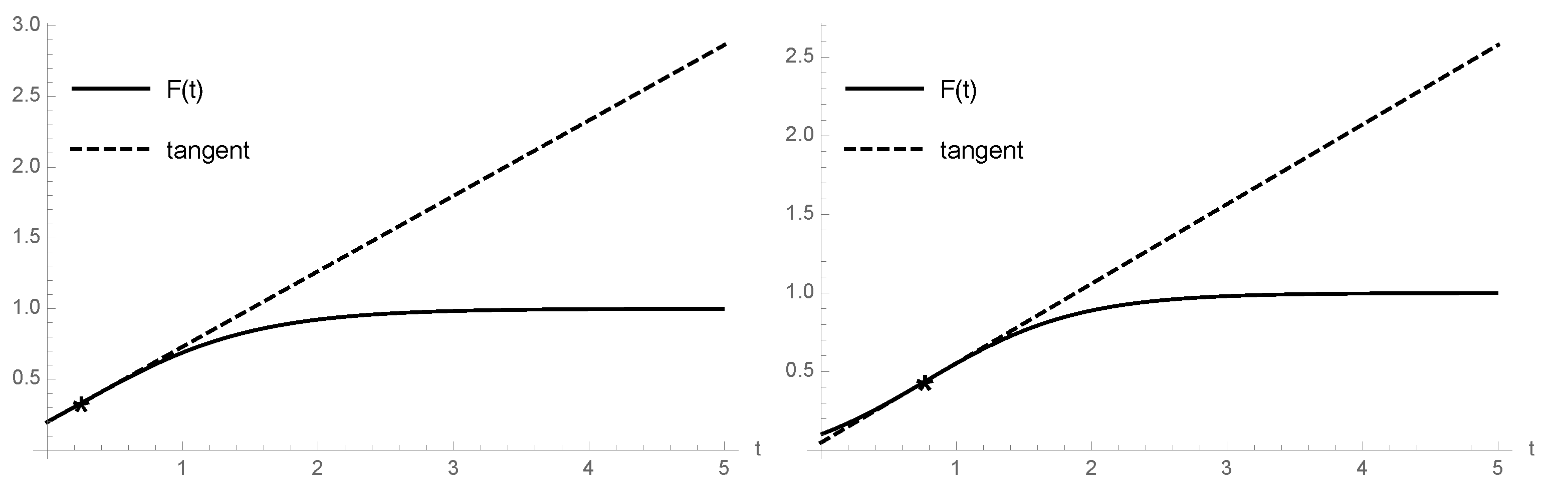
2.2. The Inflection Point

Let us now focus on the inflection point of the function $F\left(t\right)$. In the context of population dynamics, the analysis of the inflection time is of great interest, since this point represents the instant at which the growth rate of the function is maximum. From (1), by evaluating the second derivative of $F\left(t\right)$, one obtains the following results. For $-1<\epsilon \le 0$, the function $F\left(t\right)$ has downward concavity for any $t\ge 0$, whereas, if $0<\epsilon <1$, the curve $F\left(t\right)$ is sigmoidal with an inflection point at

$$t_F=\frac{1}{1+\epsilon }log\left(\frac{2\epsilon }{C(1-\epsilon )}\right).$$

(8)

Note that $t_F\ge 0$ if, and only if, $\epsilon >C/(2+C)$. In this case, the size of the population at the inflection point $t_F$ is given by

$$F\left(t_F\right)=\frac{3}{4}-\frac{1}{4\epsilon }\ge 0.$$

As performed in similar studies, one can approximate the behavior of the curve in proximity to the inflection point by the tangent line. With this aim, let us now compute the maximum specific growth rate $\mu$, which is defined as the slope of the tangent to the curve $F\left(t\right)$ at the inflection point $t_F$. Hence, if $\epsilon >C/(2+C)$, one has

$$\mu :={\left.\frac{\mathrm{d}}{\mathrm{d}t}F\left(t\right)\right|}_{t=t_F}=\frac{{(1+\epsilon )}^2}{8\epsilon },$$

so that the line tangent to the curve $F\left(t\right)$ at the inflection point has the following expression:

$$y=\frac{1}{8\epsilon }\left[{(1+\epsilon )}^{2}t-2(1-3\epsilon )-(1+\epsilon )log\left(\frac{2\epsilon }{C(1-\epsilon )}\right)\right].$$

As a consequence, the lag time $\lambda$, which denotes the intercept with the t-axis of this tangent, is given by

$$\lambda =\frac{2(1-3\epsilon )}{{(1+\epsilon )}^2}+\frac{1}{1+\epsilon }log\left(\frac{2\epsilon }{C(1-\epsilon )}\right).$$

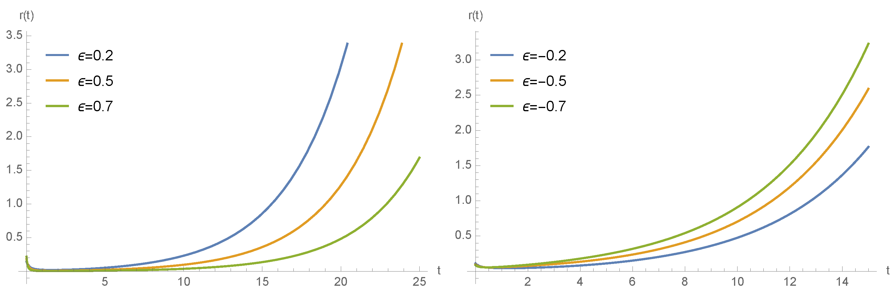
We note that the lag time represents the initial time of an ideal growth curve, which increases linearly at a constant rate given by the maximum specific growth rate and reaches the same size of the original population at the inflection point. In Figure 5, we show the function $F\left(t\right)$ and the corresponding tangent at the inflection point $t_F$ for various choices of the parameters.

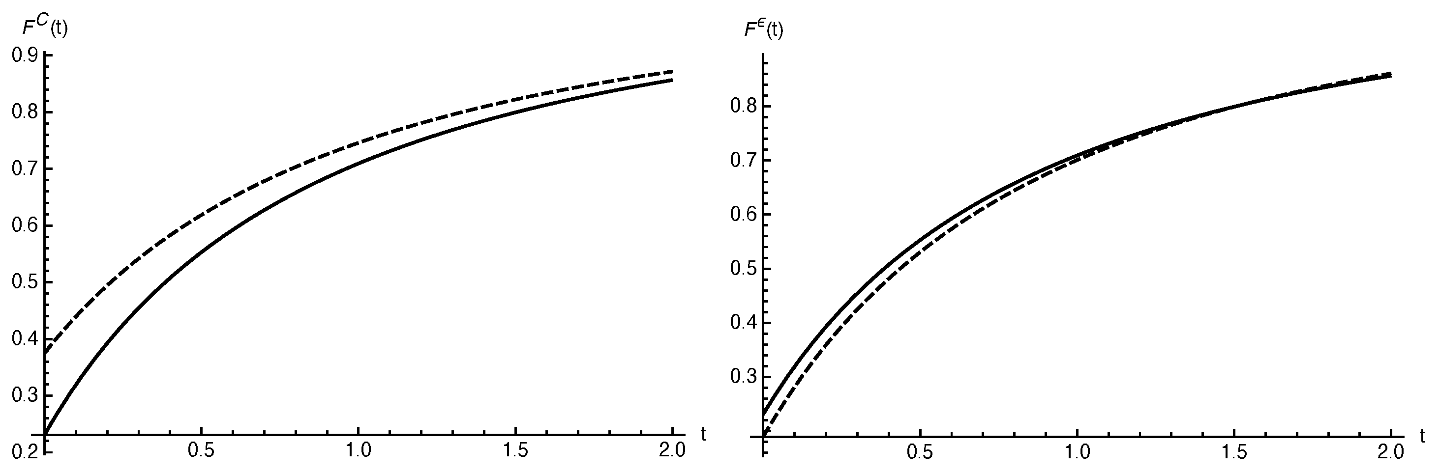
2.3. Sensitivity Analysis

In this section, we analyze how the perturbations on the parameters $C>1$ and $-1<\epsilon <1$ involved in the model influence the behaviour of $F\left(t\right)$. In the following, we denote this function by $F^{\nu }$ to emphasize the dependence on a generic parameter $\nu$. Specifically, starting from Equation (1), we expand $F^{\nu +\eta }$ in a Taylor series evaluated at $\nu$, with $\eta >0$, for $\nu =C$ and $\nu =\epsilon$.

• Perturbation on C

  $$F^{C+\eta }-F^C\approx \eta \frac{(1-{\epsilon }^2)e^{(1+\epsilon )t}}{{\left[2\epsilon +(1-\epsilon )C{e}^{(1+\epsilon )t}\right]}^2}.$$
  The latter term is positive for all $t\ge 0$.
• Perturbation on $\epsilon$

  $$F^{\epsilon +\eta }-F^{\epsilon }\approx \eta \frac{2-C{e}^{(1+\epsilon )t}[2+({\epsilon }^2-1)t]}{{\left[2\epsilon +(1-\epsilon )C{e}^{(1+\epsilon )t}\right]}^2}.$$

  (9)
  The sign of the right-hand side of (9) is equal to that of the function

  $$h\left(t\right):=2-C{e}^{(1+\epsilon )t}[2+({\epsilon }^2-1)t],t\ge 0.$$
  For $C>1$, we have $h\left(0\right)=2(1-C)<0$, the first derivative $h^{\prime }\left(t\right)$ is negative for all $t>0$, and ${lim}_{t\to +\infty }h\left(t\right)=-\infty$; therefore, from the continuity of h, we have $h\left(t\right)<0$ for all $t\ge 0$. Hence, the right-hand side of (9) is negative for all $t\ge 0$.

As an example, in Figure 6, we show the curve $F\left(t\right)$ and the effect of the perturbation $\eta =0.1$ on the parameter C (on the left) and on $\epsilon$ (on the right).

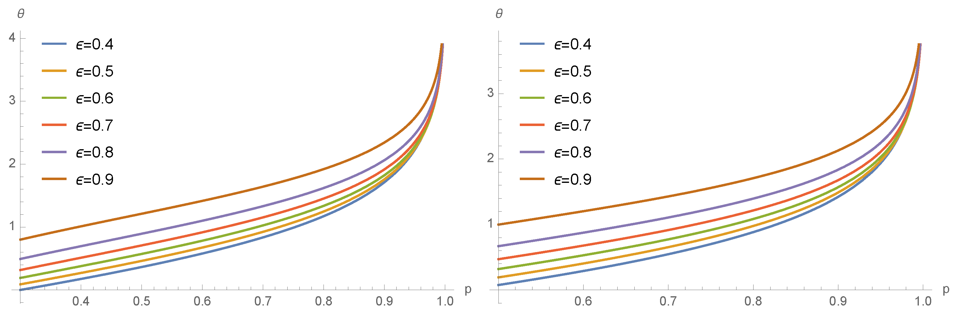
2.4. Threshold Crossing Time

In many real contexts, it is of interest to study the time spent by the growth function below (or above) a specific threshold. Indeed, such a boundary may represent a critical value related to the dynamics of the modeled population. Hence, in this section, we focus on analysis of the first-crossing-time of the function $F\left(t\right)$ through a specific constant boundary representing a percentage $p\in (0,1)$ of the whole population. In more detail, we consider $\theta$ defined as follows

$$\theta =\theta \left(p\right):=inf\{t\ge 0:F(t)=p\}.$$

(10)

Hence, by recalling (1), the equation $F\left(\theta \right)=p$ yields

$$\begin{array}{cc}\hfill \theta & =\frac{1}{1+\epsilon }log\left(\frac{1-\epsilon +2p\epsilon }{(1-\epsilon )C(1-p)}\right)\hfill \\ \hfill & =t_F+\frac{1}{1+\epsilon }log\left(\frac{1-\epsilon +2p\epsilon }{2\epsilon (1-p)}\right),\hfill \end{array}$$

where the last equality follows from (8). By Equation (1), we have that $F\left(t\right)$ is a continuous function. Hence, due to Remark 1, the existence of $\theta$ is guaranteed if p is larger than the initial proportion of burned individuals. Indeed, recalling (3), it follows that $\theta >0$ if, and only if,

$$p>F\left(0\right)\equiv \frac{C-1}{C+\frac{2\epsilon }{1-\epsilon }}\ge 0,$$

and $\theta >t_F$ if, and only if, $p>\frac{3\epsilon -1}{4\epsilon }$. In Figure 7, the first-crossing-time $\theta$ is shown for different choices of the parameters. Note that $\theta$ is increasing both with respect to p and $\epsilon$, with ${lim}_{p\to 1}\theta \left(p\right)=+\infty$ and ${lim}_{\epsilon \to 1}\theta \left(p\right)=+\infty$.

The determination of $\theta \left(p\right)$ deserves attention since it represents the time required for the information to reach the percentage p of the population. In this respect, it is useful to investigate some cases for given choices of p. Due to (10), one has

$$\theta \left(p_2\right)-\theta \left(p_1\right)=\frac{1}{1+\epsilon }log\frac{(1-p_1)(1-\epsilon +2p_2\epsilon )}{(1-p_2)(1-\epsilon +2p_1\epsilon )},$$

so that, for instance,

$$\frac{\theta (3/4)-\theta (1/2)}{\theta (1/2)-\theta (1/4)}=\frac{log(2+\epsilon )}{log(3/(2-\epsilon \left)\right)}>1.$$

This implies that, whatever the value of $\epsilon$, the time required for increasing the informed percentage from $1/2$ to $3/4$ is greater to that required for increasing the same from $1/4$ to $1/2$.

Remark 3.

We recall that the growth function $F\left(t\right)$, given in (1), represents the fraction of burned individuals in the population. Hence, assuming that the population size is $N>1$, due to (1), the function

$$\tilde{F}\left(t\right):=N·F\left(t\right)=N·\frac{Cexp\left((1+\epsilon )t\right)-1}{Cexp\left((1+\epsilon )t\right)+\frac{2\epsilon }{1-\epsilon }},t\ge 0,$$

(11)

with $C\ge 1$ and $-1<\epsilon <1$, denotes the (approximated) total number of burned individuals at time t. Making use of Equation (5), it is easy to see that the function $\tilde{F}\left(t\right)$ satisfies the following Malthusian-type equation:

$$\frac{\mathrm{d}}{\mathrm{d}t}\tilde{F}\left(t\right)=\xi \left(t\right)\tilde{F}\left(t\right),t\ge 0,\tilde{F}\left(0\right)=N·F\left(0\right),$$

(12)

where $\xi \left(t\right)$ is given in (6). Due to (11), the main difference between $F\left(t\right)$ and $\tilde{F}\left(t\right)$ lays in the carrying capacity. Indeed, the carrying capacity for $F\left(t\right)$ is 1, whereas the carrying capacity for $\tilde{F}\left(t\right)$ is equal to the population size N. Since N can be quite large, this will allow us to consider stochastic processes with infinite state-space as a stochastic counterpart of the considered growth model, as specified in Section 3 and Section 4 below.

3. A Special Time-Inhomogeneous Linear Pure Birth Process

The introduction of stochasticity in growth equations can be performed in several ways. A classical approach in this framework is based on the variation of one or more parameters in the given model (see, for instance, the review article by Karim et al. [36] on logistic growth equations). However, the need for data-driven and applicable models in stochastic growth equations implies the criteria leading to stochastic processes whose mean value is identical to the underlying growth curve. Hence, aiming to introduce a stochastic counterpart of the model considered in (11), with $F\left(t\right)$ given in (1), we focus on a description of a continuous-time Markov chain having a countable state-space. The latter assumption is justified by the fact that the size of the population considered in Remark 3 may be large; consequently, the carrying capacity of $\tilde{F}\left(t\right)$ may be large as well. For this reason, we refer to the growth function $\tilde{F}\left(t\right)$ rather than $F\left(t\right)$. Moreover, in order to describe the effect of environmental perturbations that lead to fluctuations in the experimentally observed growth curves, hereafter, we introduce a suitable point process whose mean exhibits the same behavior shown by $\tilde{F}\left(t\right)$. This approach has been followed in similar growth schemes. However, in contrast to cases in which the sample-paths of the relevant processes follow skip-free behavior (as seen e.g., in Section 4 of [6], Section 3 of [3], Section 5 of [5] and Sections 4 and 5 of [7]), we consider a process having non-decreasing sample-paths, so that the analogy with the strictly increasing function $\tilde{F}\left(t\right)$ is more tight. Specifically, we refer to an inhomogeneous linear pure birth process $\left\{M\right(t);t\ge 0\}$ having state space $S:=\{y,y+1,y+2,\cdots \}$, for a fixed $y\in \mathbb{N}$, with birth rates

$${\lambda }_n\left(t\right):=\underset{h\to 0^{+}}{lim}\frac{1}{h}\mathsf{P}[M(t+h)=n+1|M\left(t\right)=n]=n\lambda \left(t\right),n\in S.$$

(13)

Here, $\lambda \left(t\right)$ is a positive function, integrable on any interval $(0,t)$ for $t>0$, that represents the individual birth rate. The probability of a single birth during an infinitesimal time-interval after time t is proportional to the current size of the population and to the time-dependent rate $\lambda \left(t\right)$ representing the individual birth rate at time t. In this context, $M\left(t\right)$ describes the number of burned individuals, i.e., the number of individuals reached by the rumor within $[0,t]$, and the births correspond to the individual burnings.

The transition probabilities of $M\left(t\right)$ are given by (see [1])

$$P_{y,x}\left(t\right)=\mathsf{P}[M\left(t\right)=x|M\left(0\right)=y]=\left(\genfrac{}{}{0pt}{}{x-1}{y-1}\right)e^{-y\mathsf{\Lambda }\left(t\right)}{\left(1-e^{-\mathsf{\Lambda }\left(t\right)}\right)}^{x-y},t\ge 0,x\in S,$$

(14)

where

$$\mathsf{\Lambda }\left(t\right):={\int }_0^t\lambda \left(s\right)\mathrm{d}s,t\ge 0$$

(15)

is the individual cumulative birth rate over $[0,t]$. In this case, the probability generating function has the following expression (see [1]), for any $0\le z\le 1$ and $t\ge 0$,

$$G(z,t)=\sum _{x=0}^{+\infty }{P}_{yx}\left(t\right)z^x={\left\{1-(z-1){\left[(z-1)\varphi \left(t\right)-\psi \left(t\right)\right]}^{-1}\right\}}^y,$$

(16)

where

$$\psi \left(t\right):=exp\left(-{\int }_0^t\lambda \left(\tau \right)\mathrm{d}\tau \right),\varphi \left(t\right):={\int }_0^t\lambda \left(\tau \right)\psi \left(\tau \right)\mathrm{d}\tau ,t\ge 0.$$

(17)

We note that $\psi \left(t\right)$ and $\varphi \left(t\right)$ are two auxiliary functions which allow expression of the probability generating function $G(z,t)$ in a more compact manner. Thanks to Equation (16), it is possible to show that

$$\begin{array}{cc}\hfill & {\mathsf{E}}_y\left(t\right):=\mathsf{E}\left[M\left(t\right)\left|M\right(0)=y\right]=\frac{y}{\psi \left(t\right)},\hfill \\ \hfill & {\mathsf{Var}}_y\left(t\right):=\mathsf{Var}\left[M\left(t\right)\left|M\right(0)=y\right]=y\frac{\psi \left(t\right)+2\varphi \left(t\right)-1}{{\psi }^2\left(t\right)},\hfill \end{array}$$

(18)

for $t\ge 0$. The following proposition provides a necessary and sufficient condition so that the conditional mean of the process $M\left(t\right)$ equals the growth curve $\tilde{F}\left(t\right)$ specified in (11).

Proposition 1.

The linear birth process $M\left(t\right)$ with transition rates specified in Equation (13) and initial value $M\left(0\right)=y$, has a conditional mean

$${\mathsf{E}}_y\left(t\right)=\tilde{F}\left(t\right),t\ge 0$$

if, and only if,

$$\lambda \left(t\right)=\xi \left(t\right),t\ge 0$$

(19)

where $\xi \left(t\right)$ is given in (6) for

$$C=\frac{2\epsilon y+N-N\epsilon }{(1-\epsilon )(N-y)}\ge 1,$$

(20)

with $N\in S\setminus \left\{y\right\}$.

Proof. 

The result follows immediately considering that ${\mathsf{E}}_y\left(t\right)$ satisfies the differential equation

$$\frac{\mathrm{d}}{\mathrm{d}t}{\mathsf{E}}_y\left(t\right)=\lambda \left(t\right){\mathsf{E}}_y\left(t\right),t\ge 0,$$

with ${\mathsf{E}}_y\left(0\right)=y$, and recalling Equation (12). □

With reference to Equation (11), we recall that N represents the size of the carrying capacity, i.e., the total number of individuals that will eventually be reached by the rumor, and y is the number of individuals who know the rumor at the beginning of the spread, i.e., at $t=0$, with $y<N$. Instead, considering the linear birth process $M\left(t\right)$ with birth rates specified in Equation (13), we note that N represents the mean total number of individuals eventually reached by the rumor, i.e., ${lim}_{t\to +\infty }{\mathsf{E}}_y\left(t\right)=N$, and $y=M\left(0\right)$ is the initial state of the process $M\left(t\right)$. Note that, differently from the deterministic growth model whose initial state (3) may be equal to 0, for the stochastic process $M\left(t\right)$, we have $M\left(0\right)=y>0$.

In the following, we assume that the individual birth rate is fixed as specified in Equation (19). In this special case, $\lambda \left(t\right)$ is a decreasing and convex function that approaches 0 as $t\to +\infty$, as shown in Figure 8. Hence, due to (15), the function $\mathsf{\Lambda }\left(t\right)$ can be expressed as follows:

$$\mathsf{\Lambda }\left(t\right)=log\left(\frac{N\left[(e^{(1+\epsilon )t}-1)(\epsilon -1)N+y(\epsilon -1-2\epsilon e^{(1+\epsilon )t})\right]}{y\left[2\epsilon (y-N)+e^{(1+\epsilon )t}((\epsilon -1)N-2\epsilon y)\right]}\right),t\ge 0.$$

(21)

Clearly, due to (14), Equation (21) allows expression of the transition probabilities of $M\left(t\right)$ in a closed form under the conditions specified in Proposition 1. Moreover, the function $\mathsf{\Lambda }\left(t\right)$ has a finite limit when $t\to +\infty$, i.e.,

$$\underset{t\to +\infty }{lim}\mathsf{\Lambda }\left(t\right)=log\frac{N}{y}.$$

This can be used in Equation (14) in order to obtain the asymptotic probabilities of $M\left(t\right)$, i.e., ${lim}_{t\to +\infty }{P}_{y,x}\left(t\right)$. In Figure 9, we provide some plots of the probability $P_{y,x}\left(t\right)$ obtained by means of Equation (14).

The functions $\varphi \left(t\right)$ and $\psi \left(t\right)$ are available in closed form thanks to Equation (17). This allows us to obtain an explicit expression for the conditional variance of $X\left(t\right)$, as shown in the following proposition.

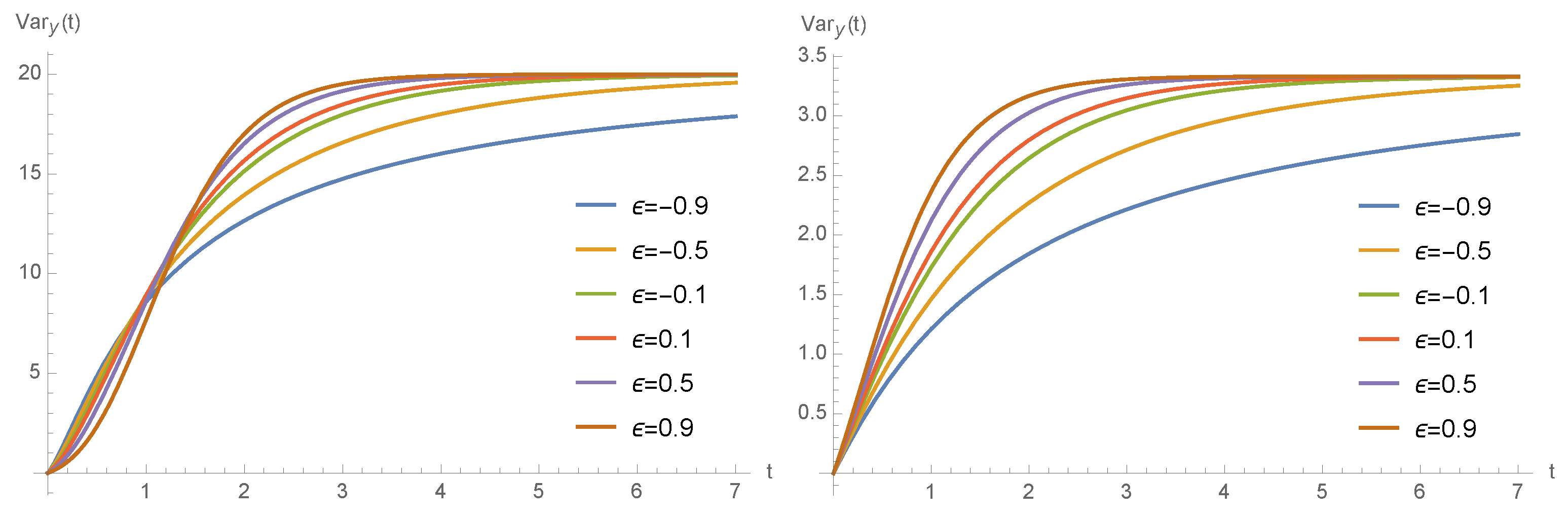
Proposition 2.

The linear birth process $M\left(t\right)$ with transition rates (13) and with individual birth rate (19), with $\xi \left(t\right)$ and C given, respectively, in (6) and (20), has conditional variance given by

$$\begin{array}{cc}\hfill {\mathsf{Var}}_y\left(t\right)& =\frac{(e^{(1+\epsilon )t}-1)N(N-y)}{y{\left(2\epsilon (N-y)+e^{(1+\epsilon )t}(N-\epsilon N+2\epsilon y)\right)}^2}\hfill \\ \hfill & \times \left[\left(N(\epsilon -1)-2\epsilon y\right)\left(e^{(1+\epsilon )t}-1\right)(\epsilon -1)N+y(-1+\epsilon -2\epsilon e^{(1+\epsilon )t})\right],t\ge 0.\hfill \end{array}$$

Proof. 

Determining $\psi \left(t\right)$ and $\varphi \left(t\right)$ by means of (17), the result, thus, follows from Equation (18) after some calculations. □

Various plots of the conditional variance ${\mathsf{Var}}_y\left(t\right)$ are given in Figure 10.

Under the assumptions of Proposition 2, it is worth noting that the variance has a finite limit for $t\to +\infty$; indeed,

$$\underset{t\to +\infty }{lim}{\mathsf{Var}}_y\left(t\right)=\frac{N(N-y)}{y}.$$

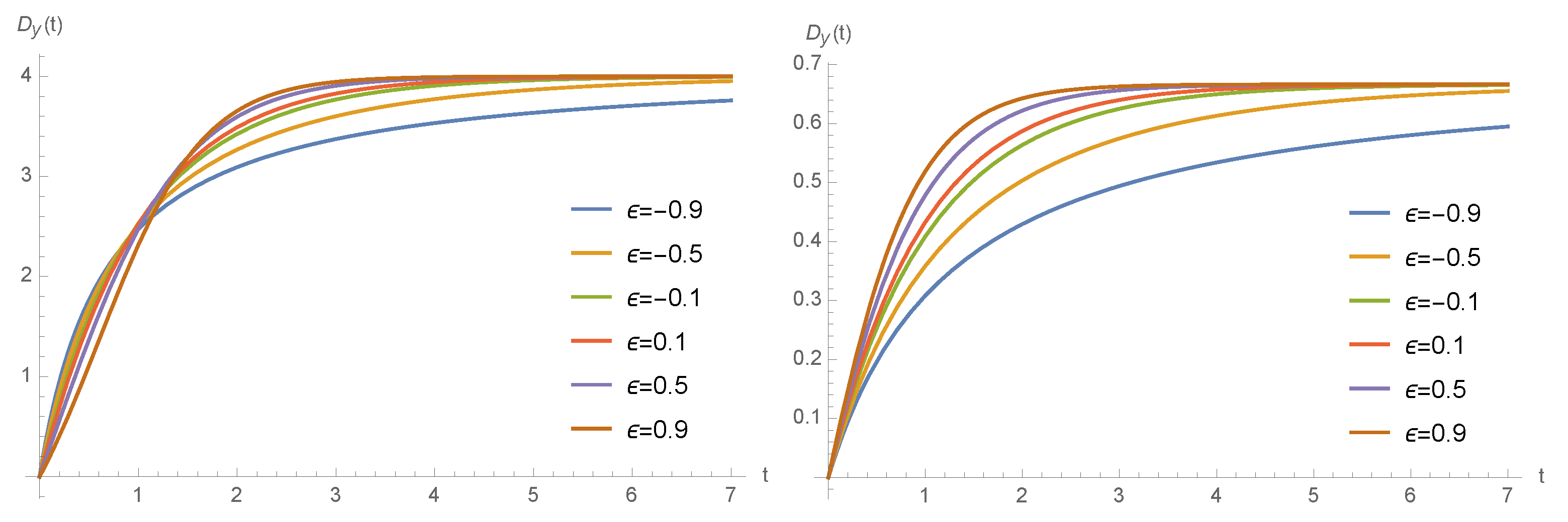
Since the conditional variance ${\mathsf{Var}}_y\left(t\right)$ has a finite limit as $t\to +\infty$, the corresponding conditional mean $E_y\left(t\right)$ is a significant index for the description of the birth process. Then, this property is found for other related quantities. Indeed, it is possible to obtain explicit expressions also for some indexes of dispersion for $M\left(t\right)$, such as the Fano factor and the coefficient of variation. In particular, when the conditions of Proposition 2 are satisfied, the Fano factor is given by

$${\mathsf{D}}_y\left(t\right):=\frac{{\mathsf{Var}}_y\left(t\right)}{{\mathsf{E}}_y\left(t\right)}=\frac{N-y}{y\left[1+\frac{(1+\epsilon )N}{(e^{(1+\epsilon )t}-1)(N-\epsilon N+2\epsilon y)}\right]},t\ge 0.$$

(22)

It is easy to show that ${\mathsf{D}}_y\left(t\right)$ is increasing with respect to t; its initial value is given by ${\mathsf{D}}_y\left(0\right)=0$ and

$$\underset{t\to +\infty }{lim}{\mathsf{D}}_y\left(t\right)=\frac{N}{y}-1>0.$$

Hence, we have that

(i)

if $y>N/2$, then the pure birth process $M\left(t\right)$ is underdispersed, i.e., ${\mathsf{D}}_y\left(t\right)<1$ for any $t\ge 0$,

(ii)

if $y<N/2$, then the pure birth process $M\left(t\right)$ is underdispersed for $t<\tilde{t}$ with

$$\tilde{t}:=\frac{1}{1+\epsilon }log\left(\frac{(1+\epsilon )Ny}{\left(N\right(1-\epsilon )+2\epsilon y)(N-2y)}+1\right),$$

and $M\left(t\right)$ is overdispersed for $t>\tilde{t}$.

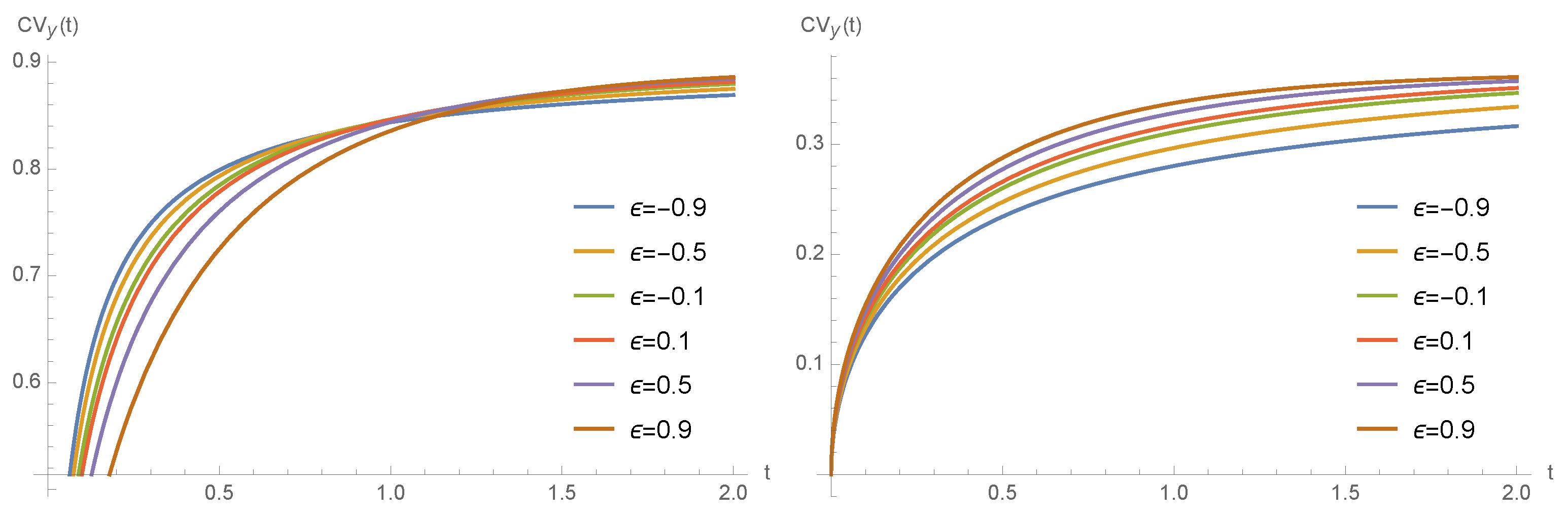
In Figure 11, some plots of the Fano factor are provided. Moreover, if the condition given in Proposition 2 is fulfilled, then the coefficient of variation ${\mathsf{CV}}_y\left(t\right):=\sqrt{{\mathsf{Var}}_y\left(t\right)}/{\mathsf{E}}_y\left(t\right)$ can be obtained in closed form for any $t\ge 0$. However, we omit the expression for brevity. Clearly, one has $C{V}_y\left(0\right)=0$. Moreover, the following limit holds

$$\underset{t\to +\infty }{lim}{\mathsf{CV}}_y\left(t\right)=\sqrt{\frac{N-y}{Ny}}>0.$$

Some plots of the coefficient of variation ${\mathsf{CV}}_y\left(t\right)$ are provided in Figure 12.

Note that the conditional variance ${\mathsf{Var}}_y\left(t\right)$, the Fano factor ${\mathsf{D}}_y\left(t\right)$, and the coefficient of variation ${\mathsf{CV}}_y\left(t\right)$ are all increasing in t, and, for large times, they are increasing also with respect to $\epsilon$. Hence, for large t and for an increasing number of initial burned individuals, the considered variability indexes attain large values. Finally, even though the expressions of the indexes obtained so far are quite cumbersome, it is worth noting that they are available in useful closed forms.

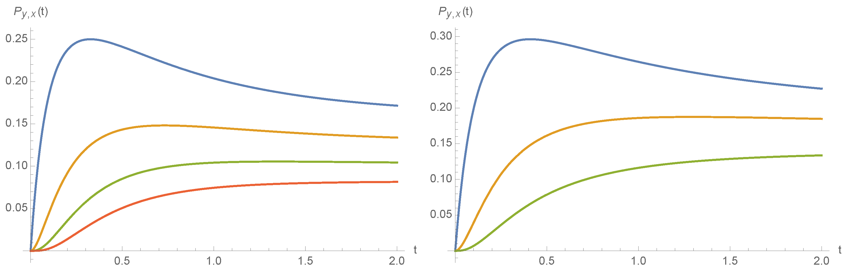
First-Passage-Time Problem

By analogy with the threshold crossing time problem considered in Section 2.4, in this section, we refer to the first-passage-time problem of the process $M\left(t\right)$. Considering the initial state $M\left(0\right)=y\in \mathbb{N}$, we fix a threshold $k\in \mathbb{N}$ with $k>y$. Consequently, the first-passage time of the process $X\left(t\right)$ through the boundary k is defined as follows

$$T_{y,k}:=inf\left\{t\ge 0:M\left(t\right)=k\right\},M\left(0\right)=y.$$

(23)

Thus, $T_{y,k}$ represents the first (random) instant in which k individuals are reached by the rumor, when the initial number of informed ones is $y>0$. The probability density function of $T_{y,k}$ is denoted by $g_{y,k}\left(t\right)$. Since the sample paths of the pure birth process $M\left(t\right)$ are non-decreasing over the state space S, it is easy to show that, for $t>0$,

$$g_{y,k}\left(t\right)=(k-1)\lambda \left(t\right)P_{y,k-1}\left(t\right)=(k-1)\lambda \left(t\right)\left(\genfrac{}{}{0pt}{}{k-2}{y-1}\right)e^{-y\mathsf{\Lambda }\left(t\right)}{\left(1-e^{-\mathsf{\Lambda }\left(t\right)}\right)}^{k-1-y},$$

(24)

with $k>y$, $\lambda \left(t\right)$ defined in Equation (19) and $\mathsf{\Lambda }\left(t\right)$ given in Equation (15). In general, the first-passage time (23) is finite w.p. less than unity. However, from (24), we have

$$\underset{N\to +\infty }{lim}\mathsf{P}(T_{y,k}<+\infty )=\underset{N\to +\infty }{lim}{\int }_0^{+\infty }{g}_{y,k}\left(t\right)\mathrm{d}t=1.$$

This is in accordance with the fact that the pure birth process with a countable state space is a suitable stochastic counterpart of the growth function $\tilde{F}\left(t\right)$ when the population size N of the model (1) is large.

Moreover, we have that $P_{y,k-1}\left(0\right)=0$, for $k-1\ne y$. Hence, due to Equations (19) and (24), the initial value of the first-passage-time probability density function is given by

$$\underset{t\to 0}{lim}{g}_{y,k}\left(t\right)=\left\{\begin{array}{cc}{\displaystyle y\lambda \left(0\right)=y\frac{C{(1+\epsilon )}^2}{(C-1)(2\epsilon +(1-\epsilon \left)C\right)},}\hfill & \mathrm{if}k=y+1\hfill \\ 0,\hfill & \mathrm{if}k>y+1.\hfill \end{array}\right.$$

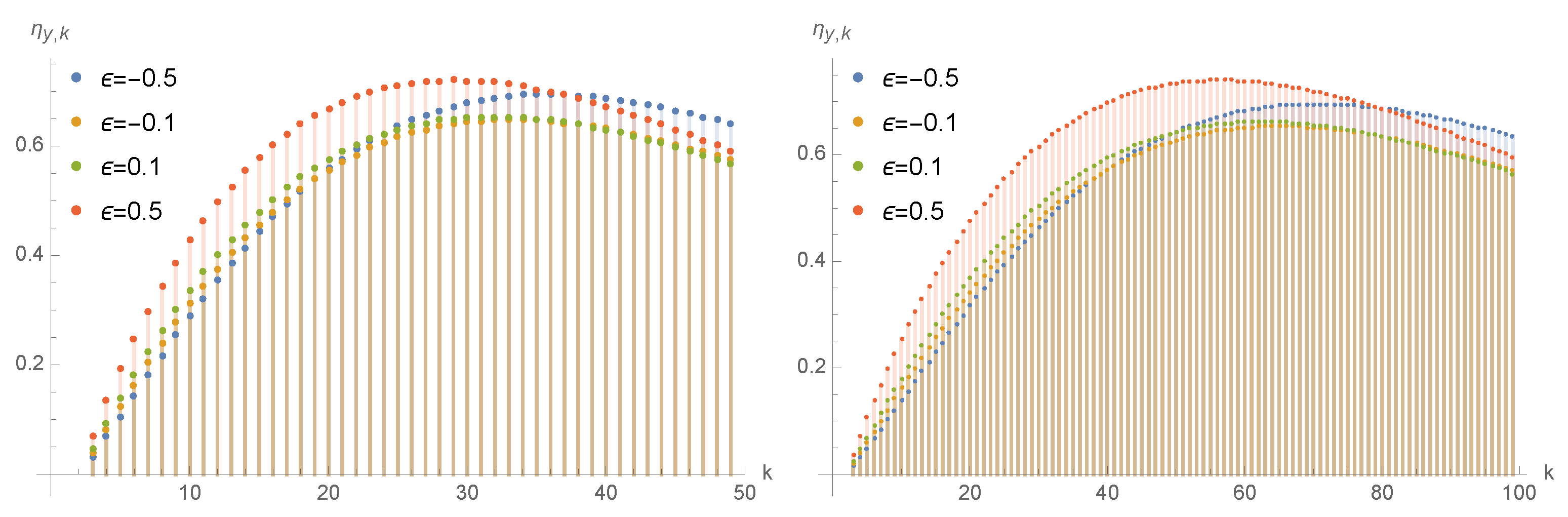
Let $\mathbb{I}$ denote the indicator function. Some plots of the expected value ${\eta }_{y,k}:=\mathsf{E}(T_{y,k}·\mathbb{I}(T_{y,k}<+\infty ))$ are given in Figure 13 for different values of the parameters. In this case, such an expectation is non-monotonic with respect to k, being increasing (decreasing) for small (large) values of k. Moreover, it is monotonic increasing with respect to $\epsilon$ for small values of k.

The discrete process considered in this section provides a suitable proposal for describing the growth of rumor spreads, thanks to the results of Proposition 1. However, when the population size N is very large, the information concerning the process $M\left(t\right)$ is not very manageable, so that the adoption of an alternative process is recommended. For instance, it is appropriate to consider a stochastic process with continuous state-space that, as seen for $M\left(t\right)$, possesses a mean which is identical to the growth curve. For this reason, in the following section, we focus on a diffusion process that will constitute an alternative tractable model for the description of the rumor spreads.

4. A Special Lognormal Diffusion Process

Let us consider a non-homogeneous diffusion process $\left\{X\right(t);t\ge 0\}$, with state-space ${\mathbb{R}}^{+}$ and infinitesimal moments

$$A_1(x,t)=\xi \left(t\right)x,A_2\left(x\right)={\sigma }^2{x}^2,t\ge 0,x\in {\mathbb{R}}^{+},$$

(25)

where $\xi \left(t\right)$ is defined in Equation (6), and $\sigma >0$. The statistical properties of $X\left(t\right)$, including the infiniteness of its state-space, make it an ideal candidate for the description of growth phenomena in the presence of high environmental variability, in agreement with Remark 3. In addition, we note that the considered non-homogeneous diffusion process can be regarded as a diffusive approximation of a special birth–death process with quadratic transition rates (see Section 5.2 of [7]). With reference to (25), note that $X\left(t\right)$ is a lognormal diffusion process with a time-dependent drift, and it is the solution of the following stochastic differential equation

$$\mathrm{d}X\left(t\right)=\xi \left(t\right)X\left(t\right)\mathrm{d}t+\sigma X\left(t\right)\mathrm{d}W\left(t\right),t>0,X\left(0\right)=X_0,$$

where $W\left(t\right)$, $t\ge 0$, is a standard Wiener process independent from the initial condition $X\left(0\right)=X_0$. By means of Itô’s formula, the resulting process can be expressed as follows

$$X\left(t\right)=X_{0}exp\left(\Xi (0,t)+\sigma W\left(t\right)\right),t\ge 0,$$

(26)

where, for $\xi \left(t\right)$ defined in (6), for $t\ge s$, one has

$$\begin{array}{cc}\hfill \Xi (s,t):& ={\int }_s^t\xi \left(\tau \right)\mathrm{d}\tau -\frac{{\sigma }^2}{2}(t-s)\hfill \\ \hfill & =log\left(\frac{2\epsilon -C{e}^{(1+\epsilon )s}(\epsilon -1)}{1-C{e}^{(1+\epsilon )s}}\right)-log\left(\frac{2\epsilon -C{e}^{(1+\epsilon )t}(\epsilon -1)}{1-C{e}^{(1+\epsilon )t}}\right)-\frac{{\sigma }^2}{2}(t-s).\hfill \end{array}$$

(27)

In both cases, if $X_0$ has a lognormal distribution ${\mathsf{\Lambda }}_1\left({\mu }_0,{\sigma }_0^2\right)$, or if $\mathsf{P}\left(X_0=x_0\right)=1$, then, the random vector ${(X\left(t_1\right),\cdots ,X\left(t_n\right))}^T$ has an n-dimensional lognormal distribution ${\mathsf{\Lambda }}_n\left(\overrightarrow{ϵ},\mathsf{\Sigma }\right)$, where $\overrightarrow{ϵ}={({ϵ}_1,\cdots ,{ϵ}_n)}^T\in {\mathbb{R}}^n$ and $\mathsf{\Sigma }={\left({\sigma }_{i,j}\right)}_{i,j}\in {\mathbb{R}}^{n\times n}$ with

$${ϵ}_i={\mu }_0+\Xi (0,t_i),{\sigma }_{ij}={\sigma }_0^2+{\sigma }^{2}min(t_i,t_j),i,j=1,\cdots ,n.$$

From the joint probability density function of ${(X\left(t_1\right),\cdots ,X\left(t_n\right))}^T$, it is possible to obtain the transition probability density function of $X\left(t\right)$ given $X\left(s\right)=y$, for $0\le s<t$. In more detail, for $x,y\in {\mathbb{R}}^{+}$ and $0\le s<t$, one has

$$\begin{array}{cc}\hfill f(x,t|y,s)& :=\frac{\mathrm{d}}{\mathrm{d}t}\mathsf{P}\left(X\left(t\right)\le x\left|X\right(s)=y\right)\hfill \\ \hfill & =\frac{1}{x\sqrt{2\pi {\sigma }^2(t-s)}}exp\left(-\frac{{\left(log(x/y)-\Xi (s,t)\right)}^2}{2{\sigma }^2(t-s)}\right),\hfill \end{array}$$

(28)

where $\Xi (s,t)$ is defined in Equation (27). It is easy to note that $\left[X\right(t\left)\right|X\left(s\right)=y]$ follows a lognormal distribution with parameters $logy+\Xi (s,t)$ and ${\sigma }^2(t-s)$, i.e.,

$$\left[X\left(t\right)\right|X\left(s\right)=y]\sim {\mathsf{\Lambda }}_1\left(logy+\Xi (s,t),{\sigma }^2(t-s)\right),s<t.$$

Since the conditional distribution of $X\left(t\right)$ is available in closed form, it is possible to obtain some of the most relevant characteristics of this process, as shown below. The conditional n-th moment of the process $X\left(t\right)$ given $X\left(s\right)=y\in {\mathbb{R}}^{+}$ for $0\le s<t$ is

$$\mathsf{E}\left(X{\left(t\right)}^n|X\left(s\right)=y\right)=y^n{\left(\frac{\left(2\epsilon -C{e}^{(1+\epsilon )s}(\epsilon -1)\right)(1-C{e}^{(1+\epsilon )t})}{\left(2\epsilon -C{e}^{(1+\epsilon )t}(\epsilon -1)\right)(1-C{e}^{(1+\epsilon )s})}\right)}^{n}exp\left(\frac{n(n-1)}{2}{\sigma }^2(t-s)\right),$$

(29)

for any $n\in \mathbb{N}$. Consequently, the unconditional n-th moment of the process $X\left(t\right)$, $t\ge 0$, can be expressed as follows

$$\mathsf{E}\left(X{\left(t\right)}^n\right)={\left(\mathsf{E}\left(X_0\right)\right)}^n{\left(\frac{\left(2\epsilon -C(\epsilon -1)\right)(1-C{e}^{(1+\epsilon )t})}{\left(2\epsilon -C{e}^{(1+\epsilon )t}(\epsilon -1)\right)(1-C)}\right)}^{n}exp\left(\frac{n(n-1){\sigma }^{2}t}{2}\right)$$

(30)

for any $n\in \mathbb{N}$. From Equations (29) and (30), one can obtain the expression of the conditional and the unconditional expected value of the process $X\left(t\right)$, i.e.,

$$\mathsf{E}\left(X\left(t\right)\left|X\right(s)=y\right)=y\frac{\left(2\epsilon -C{e}^{(1+\epsilon )s}(\epsilon -1)\right)(1-C{e}^{(1+\epsilon )t})}{\left(2\epsilon -C{e}^{(1+\epsilon )t}(\epsilon -1)\right)(1-C{e}^{(1+\epsilon )s})},t\ge s,$$

(31)

and

$$\mathsf{E}\left(X\left(t\right)\right)=\mathsf{E}\left(X_0\right)\frac{\left(2\epsilon -C(\epsilon -1)\right)(1-C{e}^{(1+\epsilon )t})}{\left(2\epsilon -C{e}^{(1+\epsilon )t}(\epsilon -1)\right)(1-C)},t\ge 0,$$

(32)

respectively. Note that both the conditional mean (31) and the unconditional mean (32) have the same form of the function $\tilde{F}\left(t\right)$ given in Equation (11), with C defined in Equation (20). Hence, the lognormal diffusion process $X\left(t\right)$, introduced in Equation (26), as the pure birth process considered in Section 3, has the conditional mean and the unconditional mean identical to the corresponding deterministic function $\tilde{F}\left(t\right)$. This allows the process $X\left(t\right)$ to describe a continuous-time rumor spread subject to random fluctuations included in the infinitesimal variance $A_2\left(x\right)$ given in Equation (25). In this way, the mean of the process corresponds to the growth function $\tilde{F}\left(t\right)$, but the sample paths of $X\left(t\right)$ are not strictly increasing. This instance is suitable to model real situations in which the diffusion of the rumor may endure abrupt slowdowns or accelerations over the time due to rough environmental perturbations.

Moreover, the conditional mode of the process $X\left(t\right)$ given $X\left(s\right)=y$, for $t\ge s\ge 0$ is given by

$$\mathsf{Mo}\left(X\left(t\right)\left|X\right(s)=y\right)=y\frac{\left(2\epsilon -C{e}^{(1+\epsilon )s}(\epsilon -1)\right)(1-C{e}^{(1+\epsilon )t})}{\left(2\epsilon -C{e}^{(1+\epsilon )t}(\epsilon -1)\right)(1-C{e}^{(1+\epsilon )s})}·exp\left(-{\sigma }^2(t-s)\right),$$

whereas the unconditional mode is

$$\mathsf{Mo}\left(X\left(t\right)\right)=e^{{\mu }_0}\frac{\left(2\epsilon -C(\epsilon -1)\right)(1-C{e}^{(1+\epsilon )t})}{\left(2\epsilon -C{e}^{(1+\epsilon )t}(\epsilon -1)\right)(1-C)}·exp\left(-{\sigma }_0^2-{\sigma }^{2}t\right),t\ge 0.$$

The $\alpha$-quantiles of the process $X\left(t\right)$ can also be determined. In more detail, the conditional $\alpha$-quantile for $t\ge s\ge 0$ is given by

$${\mathsf{C}}_{\alpha }\left(X\left(t\right)\left|X\right(s)=y\right)=y\frac{\left(2\epsilon -C{e}^{(1+\epsilon )s}(\epsilon -1)\right)(1-C{e}^{(1+\epsilon )t})}{\left(2\epsilon -C{e}^{(1+\epsilon )t}(\epsilon -1)\right)(1-C{e}^{(1+\epsilon )s})}·exp\left(z_{\alpha }\sqrt{{\sigma }^2(t-s)}\right),$$

and the unconditional $\alpha$-quantile is

$${\mathsf{C}}_{\alpha }\left(X\left(t\right)\right)=e^{{\mu }_0}\frac{\left(2\epsilon -C(\epsilon -1)\right)(1-C{e}^{(1+\epsilon )t})}{\left(2\epsilon -C{e}^{(1+\epsilon )t}(\epsilon -1)\right)(1-C)}·exp\left(z_{\alpha }\sqrt{{\sigma }_0^2+{\sigma }^{2}t}\right),t\ge 0,$$

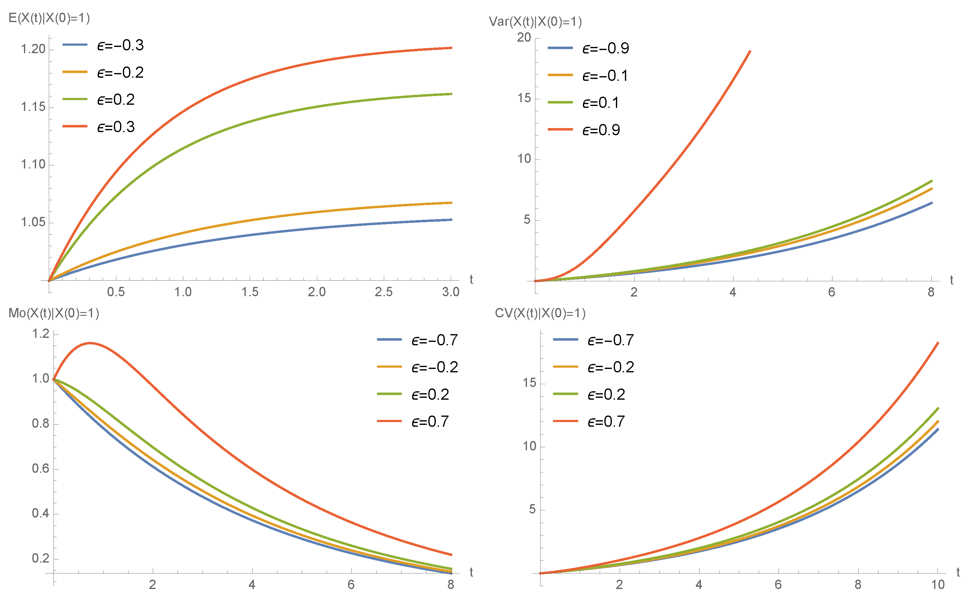
where $z_{\alpha }$ denotes the $\alpha$-quantile of a standard normal random variable. In Figure 14, we provide some plots of the conditional expected value, of the conditional variance, of the conditional mode, and of the conditional coefficient of variation of $X\left(t\right)$ given $X\left(s\right)=y$. Note that the variance and the coefficient of variation are increasing with respect to t.

4.1. First-Passage-Time Problem

This section is devoted to the study of the first-passage-time (FPT) of the diffusion process $X\left(t\right)$, defined in Equation (26), through special time-dependent boundaries. The relevance of the FPT problem for diffusion processes modeling growth phenomena is well-known in the literature. In this framework, for brevity, we limit ourselves to recalling the recent results obtained in this area in Albano et al. [37], where the FPT problem is faced for two stochastic forms of a general growth model in the presence of time-varying single or paired barriers.

Considering a continuous positive function $S\left(t\right)$, $t\ge 0$, by analogy with $T_{y,k}$ in (23), the FPT of the process $X\left(t\right)$ through the boundary $S\left(t\right)>0$ conditional on the initial state $x_0$ is defined as

$$T_{x_0}:=\left\{\begin{array}{c}inf\{t\ge t_0:X\left(t\right)>S\left(t\right)|X\left(t_0\right)=x_0\},x_0<S\left(t_0\right)\hfill \\ inf\{t\ge t_0:X\left(t\right)<S\left(t\right)|X\left(t_0\right)=x_0\},x_0>S\left(t_0\right).\hfill \end{array}\right.$$

Let us denote by $g(S\left(t\right),t|x_0,t_0)$ the probability density function of $T_{x_0}$. Determining an explicit expression for the density $g(S\left(t\right),t|x_0,t_0)$ is, in general, a hard task, since the function $g(S\left(t\right),t|x_0,t_0)$ is the solution of a Volterra integral equation (see for example Gutiérrez et al. [38]). However, it can be expressed in a closed form by considering special choices of the threshold $S\left(t\right)$. In more detail, by considering the results given in [38], if

$$S\left(t\right)=e^{A+Bt}\frac{2\epsilon +C{e}^{(1+\epsilon )t}(1-\epsilon )}{C{e}^{(1+\epsilon )t}-1},t\ge 0,$$

(33)

with $A,B\in \mathbb{R}$, then the FPT density is expressed in terms of the transition probability density function of $X\left(t\right)$, given in (28), i.e.,

$$\begin{array}{cc}\hfill g(S\left(t\right),t|x_0,t_0)& =f(S\left(t\right),t|x_0,t_0)S\left(t\right)\frac{\left|log\frac{x_0}{S\left(t_0\right)}\right|}{t-t_0}\hfill \\ \hfill & =\frac{\left|log\frac{x_0}{S\left(t_0\right)}\right|}{\sqrt{2\pi {\sigma }^2{(t-t_0)}^3}}exp\left(-\frac{{\left(log\frac{S\left(t\right)}{x_0}-\Xi (t_0,t)\right)}^2}{2{\sigma }^2(t-t_0)}\right),t\ge t_0\ge 0,\hfill \end{array}$$

(34)

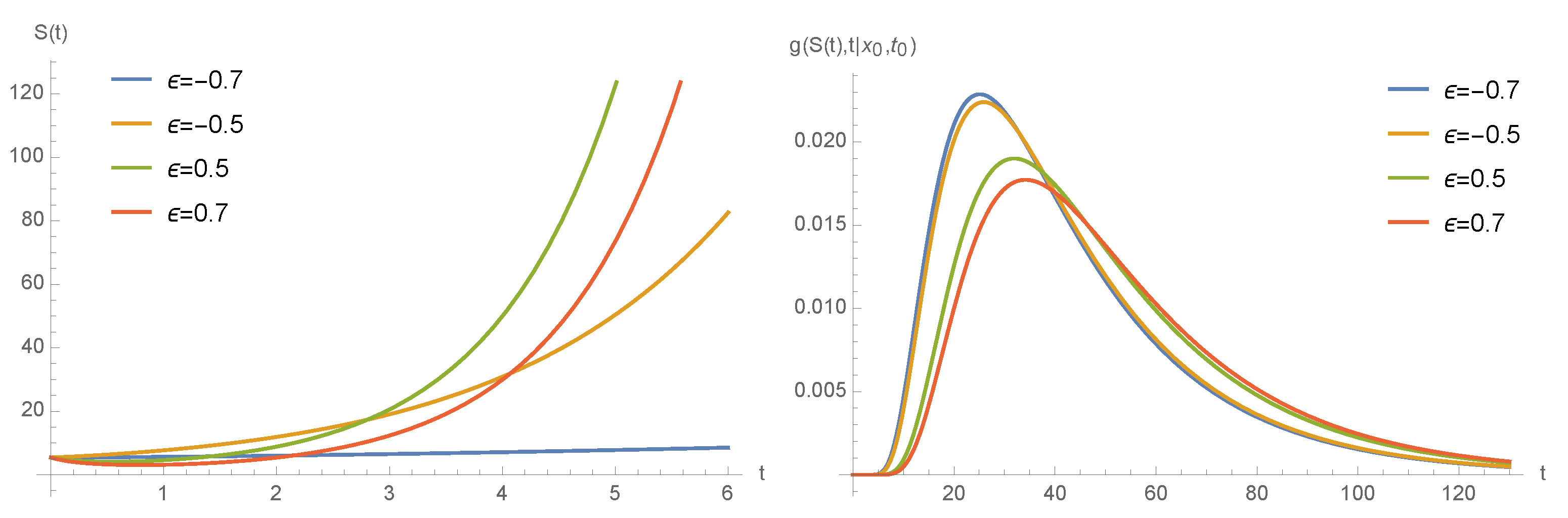
where $S\left(t_0\right)\ne x_0$ and $\Xi (s,t)$ are defined in Equation (27). Some examples of the threshold (33) and the density $g(S\left(t\right),t|x_0,t_0)$ given in (34) are plotted in Figure 15.

4.2. Comparison between the Stochastic Growth Models

We note that the birth process and the diffusion process studied, respectively, in Section 3 and Section 4, share the same mean. Hence, both processes are suitable to describe ‘randomized’ growth pertaining to the spread of a rumor among the members of a population. Consequently, it is appropriate to perform a comparison between the variances of the two processes in order to investigate their variability. To this end, we take into account the following ratio, for any $t\ge 0$

$$\begin{array}{cc}\hfill r\left(t\right)& :=\frac{\mathsf{Var}\left(X\left(t\right)\left|X\right(0)=y\right)}{{\mathsf{Var}}_y\left(t\right)}\hfill \\ \hfill & =\frac{(e^{{\sigma }^{2}t}-1){(\epsilon -1)}^{2}N{y}^3{\left(2\epsilon (y-N)+e^{(1+\epsilon )t}\left((\epsilon -1)N-2\epsilon y\right)\right)}^2}{(e^{(1+\epsilon )t}-1)(N-y)((\epsilon -1)N-2\epsilon y){(-2N+y+\epsilon y)}^2}\hfill \\ \hfill & \times \frac{1}{\left((e^{(1+\epsilon )t}-1)(\epsilon -1)N+(\epsilon -1-2e^{(1+\epsilon )t}\epsilon )y\right)\left(2\epsilon (y-N)+e^{(1+\epsilon )t}{(N(1+\epsilon )-2\epsilon y)}^2\right)},\hfill \end{array}$$

(35)

where $\mathsf{Var}\left(X\left(t\right)\left|X\right(0)=y\right)$ is the conditional variance of the diffusion process (26) and ${\mathsf{Var}}_y\left(t\right)$ is the conditional variance of the birth process introduced in Section 3. As can be deduced from Figure 16, for large values of t, the ratio $r\left(t\right)$ is greater than 1. Hence, in the presence of the same parameters and the same initial values, the variance of the birth process, with birth rate $\lambda \left(t\right)$ given in Equation (19), is smaller than the variance of the lognormal diffusion process with infinitesimal moments (25). This leads to the conclusion that the considered birth process has less variability in the modeling of the rumor spreads.

5. Conclusions

The study of fake news propagation has become crucial, especially with reference to online social networks, where control mechanisms are very difficult to implement. Several attempts have been made to provide manageable functions describing the time evolution of rumor spread. We started by considering the model introduced by San Martìn et al. [12] and we studied it from a deterministic point of view. Then, we analyzed the behavior of the curve by making different choices of the parameters, showing the flexibility of the proposed model. The stochastic counterparts of the growth function were also considered. In detail, we introduced a time non-homogeneous linear pure birth process and a lognormal diffusion process with time-dependent drift. We analyzed the conditions under which the means of such processes correspond to the deterministic growth curve. The first-passage-time problem was also addressed. Furthermore, in order to analyze the variability of the processes, we performed a comparison between their variances, noting that, for large times, the variance of the birth process was smaller than the variance of the diffusion process.

In Remark 1, it was pointed out that the carrying capacity of the model (1) is unity. This can be viewed, in a sense, as a limitation of the growth model since, in various contexts, only a fraction of the population is eventually informed by the news. However, this feature makes the model particularly appropriate for describing the diffusion of news in closed communities or in restricted environments, for example, in homogeneous groups in social networks, where it is expected that all members will be reached by the rumor.

This study should be viewed as a first step to the construction of stochastic generalization of growth models for the spreading of fake news. Clearly, the present study can be improved in the future. For instance, it will be useful to adopt stochastic schemes similar to epidemiological models, such as SIR or SIS models, to describe not only the evolution of spreaders, but also of the other components of the population. Moreover, the investigation should be extended along the following lines:

(a)

application of the considered models to real data for prediction purposes;

(b)

new growth models for the percentage of burned, i.e., informed individuals, based on suitable compartmental models;

(c)

new stochastic processes finalized to describe the diffusion of rumors subject to randomness;

(d)

constructing more general birth–death processes to model the spread of rumors also in the presence of individuals prone to forgetting the rumors;

(e)

adopting AI-based strategies for detecting disinformation and fake news.

The above sketched proposals can be the subject of future research.