Abstract
One of the most widely known probability distributions used to explain the probabilistic behavior of positive data is the log-normal (LN). Although the LN distribution is capable of adjusting data types, it is not always fully true that the model manages to adequately model the behavior of the response of interest since in some cases, the degree of skewness and/or kurtosis of the data are greater or less than those that the LN distribution can capture. Another peculiarity of the LN distribution is that it only fits unimodal positive data, which constitutes a limitation when dealing with data that present more than one mode (bimodality). On the other hand, the log-normal model only fits unimodal positive data and in reality there are multiple applications where the behavior of materials is bimodal. To fill this gap, this paper introduces a new probability distribution that is capable of fitting unimodal or bimodal positive data with a high or low degree of skewness and/or kurtosis. The new distribution is a generalization of the LN distribution. For the new proposal, its main properties are studied and the process of estimation of the parameters involved in the model is carried out from a classical perspective using the maximum likelihood method. An important feature of this distribution is the non-singularity of the Fisher information matrix, which guarantees the use of asymptotic theory to study the properties of the parameter estimators. A Monte Carlo type simulation study is carried out to evaluate the properties of the estimators and finally, an illustration is presented with a set of data related to the concentration of nickel in soil samples, allowing to show that the proposed distribution fits extremely well in certain situations.
MSC:
60E05; 62E10
1. Introduction
Until a few years ago, the modeling of positive data was limited to the use of some distributions which are characterized by being of asymmetric type, such as the gamma, Weibull, exponential and log-normal (LN) models. In geochemistry, the fundamental law enunciated by Ahrens [1], “the concentration of a chemical element in a rock has a logarithm-normal distribution”, converted to the LN distribution, one of the most used for modeling the concentration of chemical elements.The LN distribution denoted by , is defined from the transformation of the random variable , where . The model has wide applicability in studies about survival time materials in engineering sciences and some economic studies.
Another type of asymmetric distribution, used for fitting positive data, is the log-skew-normal (LSN) model introduced by Azzalini et al. [2], which is an extension of the original skew-normal (SN) distribution proposed by Azzalini [3]. From the SN model, numerous families of asymmetric distributions have been introduced and studied in detail, for example, the symmetric-asymmetric family of distributions with probability density function (PDF) given by
where , f is a symmetric PDF around zero, G is an absolutely continuous symmetric distribution function, and is a parameter that controls the asymmetry. The SN model is a special case of the model in (1), which is obtained by letting and , the PDF and the cumulative distribution function (CDF) of the normal distribution. The extension of the location-scale version of the SN model follows by applying the linear transformation , where and . This is denoted by , and the standard case by . Additional works focused on the study of the SN distribution were carried out by Azzalini and Dalla Valle [4], Henze [5] and Chiogna [6], among others.
An extension of the SN model for fitting positive data denoted by was introduced by Azzalini et al. [2]. This extension has PDF given by
where and are the PDF and CDF of the standard normal distribution, respectively, and is a parameter which controls the asymmetry and kurtosis in the model. The LSN distribution is commonly used for modeling data with skewness and kurtosis coefficients greater than the LN distribution can fit. Notice that, letting in the Equation (2), the LSN reduces to the LN model.
As an alternative to the SN model, Durrans [7] introduced another type of asymmetric distribution, called fractional order statistics model, and in much of the statistical literature referred to as alpha-power (AP) model. Properties of the AP model were studied by Gupta and Gupta [8] and Pewsey et al. [9]. The AP has PDF given by
where is a parameter that controls the skewness and kurtosis of the distribution, and F is an absolutely continuous distribution function with PDF . In the particular case of in (3), we said that the random variable Y follows the generalized Gaussian (or power-normal) distribution, and is denoted by . The extension of the location-scale of the PN model, denoted by , to the case of positive data was proposed by Martínez-Flórez et al. [10], who defined the log-power-normal (LPN) model whose PDF is given by
where and are parameters of location and scale, respectively. This model is denoted by . The LPN model contains, as a special case, the LN model when .
Contrary to the LSN model in which the information matrix is singular for the case , Martínez-Flórez et al. [10] showed that the LPN model has information matrix non-singular when . Thus, in the LPN model, statistical inference based on the theory of large samples can be carried out. The normality of the vector of maximum likelihood estimator (MLE) for the model parameters can be tested by using the likelihood-ratio statistic. The LPN was studied also by Martínez-Flórez et al. [11].
In the statistical literature, it is well known that the SN and PN models are restricted to the case of unimodal data set; so, extensions to the bimodal situations of these two models have been considered by some authors. For example, Arnold et al. [12] defined the bimodal model known as “the extended normal-asymmetric two-pieces model” (ETN), whose PDF is given by
where , and is a normalizing constant. For the ETN model, Arnold et al. [12] showed that the information matrix is singular when .
Concerning bimodal positive data, Bolfarine et al. [13] introduced the log-bimodal-skew-normal model, which is denoted by . The LBSN model is an extension of the SN distribution and is adequate for modeling bimodal positive data. The PDF of the LBSN model is given by
where , with .
Recently, Bolfarine et al. [14] extended the unimodal generalized Gaussian model of Durrans [7] to situations of bimodal asymmetric data by considering the alternative of the ETN model developed by Arnold et al. [12]. The extension of Bolfarine et al. [14], which is denoted by , has density function given by
where and are the PDF and CDF of the standard normal distribution, respectively, and, , with and . Bolfarine et al. [14] showed that the PDF in (7) is bimodal and asymmetric for values of and certain values of ; and unimodal for . Therefore, the ABPN model can be used for fitting data with a high degree of asymmetry and bimodality. For the ABPN model, the authors also showed that the information matrix is non-singular in the neighborhood of contrary to the case of the ETN model of Arnold et al. [12], whose information matrix is singular for the case . Hence, normality of the MLE for the parameters of the ABPN model can be tested by using the large sample theory together with the likelihood-ratio statistic.
In the current literature, there are few distributions for fitting bimodal positive data, and therefore, this work is focused to propose a new distribution which is adequate to fit data with this behavior. The proposed model generalizes the fundamental law of geochemistry of [1], and in addition, is more flexible than the LN, LSN and LPN models, which are contained as special cases.
The rest of the paper is organized as follows: Section 2 introduces the log-bimodal asymmetric generalized Gaussian model, and its main properties are enunciated and studied. The moment, score function, and the observed and expected information matrix are obtained. The inference for the parameters of the model is realized by using the maximum likelihood method. The results of a simulation study and its respective discussion are presented in Section 3. In Section 4, an application to a real data set consisting of samples of concentration of nickel in soil is presented to illustrate the use of the new model. Finally, a discussion about the proposed model is presented in Section 5.
2. The Log-Uni-Bi-Modal Asymmetric Generalized Gaussian Model
In this section, we introduce a new model which generalizes some distributions already known in the statistical literature for fitting positive data. This model contains two parameters that make it more flexible than the LN, LSN and LPN models, and is obtained from considering the alternative two-pieces skew-normal model for bimodal asymmetric data of Arnold et al. [12].
Definition 1.
If random variable Y is distributed with density function given by:
for ; where , and is the normalizing constant, then Y follows a log-bimodal asymmetric generalized Gaussian distribution, also called log-bimodal asymmetric power-normal (LABPN) distribution, with parameter . We use the notation .
In density function (8), is an asymmetry parameter, is a shape parameter, is a location parameter and is a scale parameter.
Although the new distribution is a little more complicated than the existing methodologies, this does not constitute a limitation in its applicability. On the one hand, the main benefit of this new proposal is the possibility of fitting positive data that present bimodality and a high degree of asymmetry and kurtosis that cannot be captured by existing models in the current literature. On the other hand, the existence of statistical packages today facilitates their implementation in practical terms.
From Definition 1, some special cases of the LABPN model are followed by letting specific values of the parameters. For example, when and the LN model follows; for , the LSN model is obtained; and, if and the LPN model follows. Finally, when , then . These results are presented in the following properties:
Property 1.
If , then , where LN denote the log-normal distribution.
Property 2.
If , then , where LN denote the log-skew normal distribution, see Azzalini et al. [2].
Property 3.
If and for all , then , where LN denote the log-skew normal distribution, see Martínez-Flórez et al. [10].
Property 4.
If , then , where LN denote the log-skew normal distribution, see Arnold et al. [12].
Differentiating the density function regarding y, we have that the derivative of is null at
where . Now, for such that , we have
and for , such that , we have
Therefore, for and certain values of satisfying
we have a log-bimodal model. Figure 1 reveals how the parameters and control the skewness, kurtosis and shape of the LABPN model.
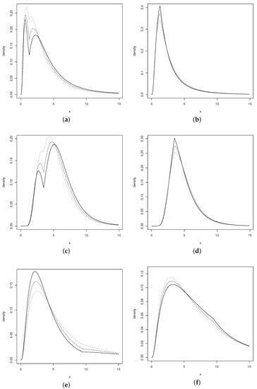
Figure 1.
PDF of the LABPN model with parameter , for: (a) with (solid line), 2.5 (dashed line), 1.75 (dotted line); (b) with (solid line), 0.5 (dashed line), 0.75 (dotted line); (c) with (solid line), 2.5 (dashed line), 1.75 (dotted line); (d) with (solid line), 0.5 (dashed line), 0.75 (dotted line); (e) with (solid line), 2.5 (dashed line), 1.75 (dotted line) and (f) with (solid line), 0.5 (dashed line), 0.75 (dotted line).
2.1. Moments
The moments of the random variable Y with LABPN distribution do not have explicit form; however, the rth moment for the standard case of the LABPN model, that is, and , which is denoted by , can be obtained by using the formula:
where , . Thus, the rth moment of can be obtained from the expression:
The following result is similar to that given for the LN, LSN and LPN models.
Property 5.
For all , the moment-generating function (MGF) of the random variable does not exist.
Proof.
The result is obvious for and , since this corresponds to the case of the LN model. For , the LSN model follows and for and for all , we have the case of the LPN model.
For (without loss of generality, we took and ), we have by definition
Letting , it follows for that
see Lin and Stoyanov [15]. In addition, by letting , we get
then, if it follows that and , where it is obtained that ; therefore, for
we conclude that . On the other hand, following Arnold and Lin [16],
we have for , and , the approximation
therefore, when , we have for fixed that
from which we can conclude that Thus, for all and , the variable random Y does not have MGF when . Therefore, does not exist, and the proof is completed. □
2.2. Statistical Inference
Given a random sample of size n, such that, , with , the log-likelihood function for the parameter can be written as
where , for . The corresponding score functions, obtained by taking the first derivative of the log-likelihood function, are given by
2.3. Observed Information Matrix
The elements of the observed information matrix are obtained by multiplying by -1 the second partial derivatives of the log-likelihood function regarding the parameters, by using the expression
with , , and . These elements are presented in detail in Appendix A.
2.4. Expected Information Matrix
Under the assumption that the regularity conditions are satisfied, the elements of the expected information matrix can be calculated by multiplying by , the expected value of the corresponding elements of the observed information matrix, that is,
In Appendix A, the explicit expressions of the elements of the expected information matrix are presented. The expectations of the expressions involved in the components of the information matrix must be calculated numerically. In the particular case where and , so that
is the density function of the LN model of location-scale version, the information matrix becomes
whose determinant , then the information matrix is non-singular in the neighborhood of and , that is, for the LN model. This is not the case for the model of Azzalini and Dalla Valle [4] for which the Fisher information matrix is singular in the neighborhood of . Furthermore, the upper sub-matrix of size corresponds to the Fisher information matrix of the LN model. Therefore, for n large
is consistent and has asymptotic normal distribution with covariance matrix . Inferences based on confidence intervals and hypothesis testing for the location, scale and shape parameters can be realized by using sampling properties for large samples of the MLE.
3. Simulation Study
This section presents a Monte Carlo simulation study, which was carried out with the objective of evaluating the behavior of the maximum likelihood estimators for the LABPN distribution.
For this simulation, the maxLik function of the statistical software R Development Core Team [17], version 4.2.3 was used and data from the LABPN distribution were generated, considering the values of the parameters: and , and different values of the parameters and .
For each scenario, 5000 random samples from the LABPN distribution were generated with the sample sizes and 500. As quality measures to evaluate the behavior of the MLEs; the bias and the mean square error (MSE) were used. These measurements were calculated as
and
where is the estimate of for the ith sample. The results of the simulation study are presented in the Table 1.

Table 1.
Bias and mean square error (MSE) of maximum likelihood estimates.
From the table, it can be seen that in general, as the sample size increases, the bias and the MSE of all parameter estimators tend to decrease and they approach zero. Thus, MLEs are asymptotically consistent and large-sample theory can be used to perform interval estimation of parameters as well as hypothesis testing based on likelihood ratio statistics.
4. Application to the Nickel Content in the Soil Data
For the illustration, we use a data set which was previously analyzed by Bolfarine et al. [13], who fitted the LBSN model. The data consists of 86 samples of nickel content (in Ni(g g)) in soil samples analyzed at the Department of Mines of the University of Atacama, Chile. The descriptive statistics for this data set are: , , , , and . For this same data set, the skewness and kurtosis coefficients of the logarithm of the nickel content for the 86 samples were also calculated, which were and , respectively; therefore, the assumption that the logarithm of the nickel content follows an LN model is inadequate.
Bolfarine et al. [13] found that the LBSN model fitted the nickel content data better than the LN model. As an alternative to the LBSN model, we fitted the LABPN model. To compare our proposal, we also fitted the LN and LSN Azzalini et al. [2] models. The MLEs of the fitted models, which were obtained numerically using the optimal function of the statistical package [17], are presented in the Table 2 with the respective standard errors in parentheses. For obtaining the parameter estimates, we used the optim function from the [17] package.
Table 2.
Estimated parameters (standard error) for the LN, LSN, LBSN and LABPN models.
To compare the fitted models, we computed the estimated values of the AIC Akaike [18], which is given by , Schwarz [19], and the modified AIC criterion [20], typically called the consistent AIC, namely, where k is the number of parameters for the considered model. The best model is the one with the smallest AIC (or BIC or CAIC). According to the AIC, BIC and CAIC statistics, the best models are the LBSN and LABPN.
The bimodality hypothesis can also be formally tested from the system of hypotheses
which is equivalent to compare the LSN and LABPN models. Since the Fisher information matrix is non-singular, we used the likelihood-ratio statistic, namely,
where is the likelihood function.
After substituting the estimated values of the parameters, we have
which is greater than the critical value of the chi-squared distribution, . This result leads to the rejection of the null hypothesis; therefore, we conclude that the LABPN model fits best the nickel concentration data.
To compare the LN model with the LABPN model, we considered the system of hypotheses
which can be tested by using the likelihood-ratio statistic given by
Considering the estimated values, we get , which is greater than the critical value of the chi-square distribution with two degrees of freedom, . Again, we rejected the null hypotheses , and we concluded that the LABPN model fits the nickel content data better than the LN model.
Now, to compare the LBSN and LABPN models, it is necessary to consider a test for non-nested models. Thus, we suppose that and are the corresponding non-nested densities to be compared. To test the hypothesis of no differences between these densities, that is,
Vuong [21] proposed the likelihood-ratio statistic given by
where
is an estimator for the variance of . One can show that, under , if , then
The null hypothesis of equivalence of the models is rejected at significance level in favor of the LABPN model, that is, better fit (or worse fit) compared to the LBSN model, if (or ). For the nickel concentration data, we obtained , which is less than the critical value ; therefore, there are no statistical differences between the LBSN and LABPN models. In this way, the LABPN model is a useful alternative to fit the nickel concentration data. Figure 2 shows the fitted densities and QQplot plots for the LSN and LABPN models. These plots also show evidence that the LABPN model fits better than the other considered models. The QQplot in Figure 2c also shows that the LABPN model has a good fit.
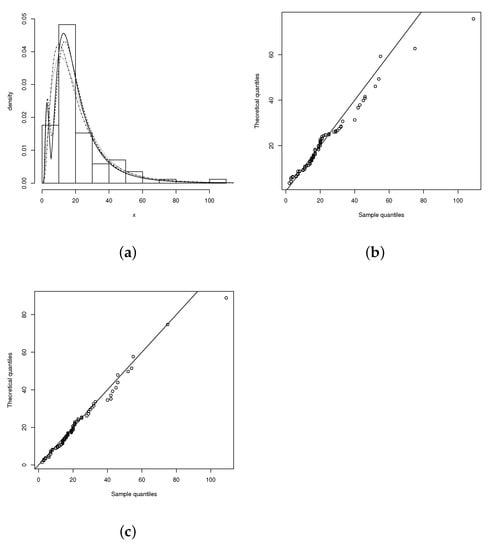
Figure 2.
(a) Histogram for the nickel concentration variable. Densities fitted by maximum likelihood: LN (dotted-dashed line), LSN (dotted line), BLSN (dashed line) and LABPN (solid line), (b) QQplot LSN and (c) QQplot LABPN.
5. Concluding Remarks
In this work, a new family of parametric distributions capable of fitting unimodal and bimodal positive data is introduced. The main properties of the new family were studied. This new family is obtained by considering the Arnold et al. [12] and Durrans [7] models and extends some existing models in the literature, among them, the log-normal, log-skew norm, log-bimodal-skew-normal and log-bimodal-power-normal. This new distribution is also very flexible and can fit unimodal and bimodal data with high (or low) degrees of skewness and kurtosis. To obtain the estimates of the parameters in the model, a classical approach was considered by using the maximum likelihood method together with iterative Newton–Raphson algorithms for the optimization of the likelihood function. The score functions were presented and the Fisher information matrix was shown to be non-singular, which allows statistical inference to be carried out through the theory of large samples and the use of likelihood-ratio statistics. The applicability of the new family was illustrated by considering a data set corresponding to nickel content in soil samples. The results showed better fit of the proposed family compared to other existing models in the literature.
Author Contributions
Conceptualization, G.M.-F. and R.T.-F.; methodology, G.M.-F., R.T.-F. and H.B.; software, G.M.-F. and R.T.-F.; validation, G.M.-F., R.T.-F. and H.B.; formal analysis, G.M.-F. and R.T.-F.; investigation, G.M.-F. and R.T.-F.; resources, G.M.-F. and R.T.-F.; data curation, G.M.-F. and R.T.-F.; writing—original draft preparation, G.M.-F. and R.T.-F.; writing—review and editing, G.M.-F., R.T.-F. and H.B.; visualization, G.M.-F. and R.T.-F.; supervision, G.M.-F. and R.T.-F.; project administration, G.M.-F. and R.T.-F.; funding acquisition, G.M.-F. and R.T.-F. All authors have read and agreed to the published version of the manuscript.
Funding
The research of G. Martinez-Flórez and R. Tovar-Falón was supported by Fondo de Investigación de la Vicerrectoría de Investigación, Universidad de Córdoba, Colombia.
Institutional Review Board Statement
Not applicable.
Informed Consent Statement
Not applicable.
Data Availability Statement
Details about available data are given in Section 3.
Acknowledgments
G. Martínez-Flórez and R. Tovar-Falón acknowledge the support given by Universidad de Córdoba, Montería, Colombia.
Conflicts of Interest
The authors declare no conflict of interest.
Appendix A. Information Matrix Elements
If the elements of the observed information matrix are denoted by , , then you have to
where . After making some calculations, the elements of the expected information matrix are given by
where and .
References
- Ahrens, L.H. The lognormal distribution of the elements (A fundamental law of geochemistry and its subsidiary). Geochim. Cosmochim. Acta 1954, 5, 49–73. [Google Scholar] [CrossRef]
- Azzalini, A.; Cappello, D.; Kotz, S. Log-skew-normal and log-skew-t distributions as models for family income data. J. Income Distrib. 2002, 11, 12–20. [Google Scholar] [CrossRef]
- Azzalini, A. A class of distributions which includes the normal ones. Scand. J. Stat. 1985, 12, 171–178. [Google Scholar]
- Azzalini, A.; Dalla Valle, A. The multivariate skew-normal distribution. Biometrika 1996, 83, 715–726. [Google Scholar] [CrossRef]
- Henze, N. A probabilistic representation of the skew-normal distribution. Scand. J. Stat. 1986, 13, 271–275. [Google Scholar]
- Chiogna, M. Some results on the scalar Skew-normal distribution. J. Ital. Stat. Soc. 1998, 1, 1–14. [Google Scholar] [CrossRef]
- Durrans, S.R. Distributions of fractional order statistics in hydrology. Water Resour. Res. 1992, 28, 1649–1655. [Google Scholar] [CrossRef]
- Gupta, R.C.; Gupta, R.D. Analyzing skewed data by power normal model. Test 2008, 17, 197–210. [Google Scholar] [CrossRef]
- Pewsey, A.; Gómez, H.W.; Bolfarine, H. Likelihood-based inference for power distributions. Test 2012, 21, 775–789. [Google Scholar] [CrossRef]
- Martínez-Flórez, G.; Bolfarine, H.; Gómez, H.W. The log-power-normal distribution with application to air pollution. Environmetrics 2014, 25, 44–56. [Google Scholar] [CrossRef]
- Martínez-Flórez, G.; Bolfarine, H.; Gómez, H.W. Asymmetric regression models with limited responses with an application to antibody response to vaccine. Biom. J. 2013, 55, 156–172. [Google Scholar] [CrossRef]
- Arnold, B.C.; Gómez, H.W.; Salinas, H.S. On Multiple Constraint Skewed Models. Stat. J. Theor. Appl. Stat. 2009, 43, 279–293. [Google Scholar] [CrossRef]
- Bolfarine, H.; Gómez, H.W.; Rivas, L. The log-bimodal-skew-normal model. A geochemical application. J. Chemom. 2011, 25, 329–332. [Google Scholar] [CrossRef]
- Bolfarine, H.; Martínez-Flórez, G.; Salinas, H.S. Bimodal symmetric-asymmetric power-normal families. Commun. Stat. Theory Methods 2018, 47, 259–276. [Google Scholar] [CrossRef]
- Lin, G.D.; Stoyanov, J. The logarithmic Skew-Normal distributions are Moment-Indeterminate. J. Appl. Probab. Trust. 2009, 46, 909–916. [Google Scholar] [CrossRef]
- Arnold, B.C.; Lin, G.D. Characterization of the skew-normal and generalized chi distributions. Sankhyā 2004, 66, 593–606. [Google Scholar]
- R Development Core Team. R: A Language and Environment for Statistical Computing; R Foundation for Statistical Computing: Vienna, Austria, 2023; Available online: http://www.R-project.org (accessed on 31 May 2023).
- Akaike, H. A new look at statistical model identification. IEEE Trans. Autom. Control. 1974, 19, 716–722. [Google Scholar] [CrossRef]
- Schwarz, G. Estimating the dimension of a model. Ann. Stat. 1978, 61, 461–464. [Google Scholar] [CrossRef]
- Bozdogan, H. Model selection and Akaike’s information criterion (AIC): The general theory and its analytical extensions. Psychometrika 1987, 52, 345–370. [Google Scholar] [CrossRef]
- Vuong, Q.H. Likelihood tatio tests for model selection and non-nested hypotheses. Econometrica 1989, 57, 307–333. [Google Scholar] [CrossRef]
Disclaimer/Publisher’s Note: The statements, opinions and data contained in all publications are solely those of the individual author(s) and contributor(s) and not of MDPI and/or the editor(s). MDPI and/or the editor(s) disclaim responsibility for any injury to people or property resulting from any ideas, methods, instructions or products referred to in the content. |
© 2023 by the authors. Licensee MDPI, Basel, Switzerland. This article is an open access article distributed under the terms and conditions of the Creative Commons Attribution (CC BY) license (https://creativecommons.org/licenses/by/4.0/).