Abstract
Nowadays, many maritime structures require precise dynamic positioning (DP) of the constructive elements that compose them. In addition, the use of preconstructed elements that are later moved to the final location has become widespread. These operations have not been automated with the risks involved in carrying out the complex operations required. To minimize these operational risks and to perform a correct DP of floating structures, a new approach based on the L1 adaptive control technique is proposed. As an example of application, a proposed L1 adaptive controller was implemented in the dynamic positioning of a floating caisson. Several simulations of the system with wave disturbances were carried out, and the results were compared with those obtained by applying other classical and advanced control techniques, such as linear quadratic Gaussian control (LQG) and model predictive control (MPC). It was concluded that the proposed L1 adaptive controller performs correct dynamic positioning and reduces the tension generated on the lines concerning the other advanced control techniques with which it was compared. This reduction in line tension leads to an important improvement due to the possibility of reducing the size of the actuators or reducing their number, with the important economic and safety repercussions that these actions entail.
MSC:
93C40
1. Introduction
Over the last few decades, new construction techniques have been used to build marine structures, such as docks, harbors, or offshore structures. One of the most prominent techniques is that in which the structure or part of the structure is fabricated in a place other than the final location and then moved to the place where it is finally sunk [1].
To carry out the displacements and subsequent sinking of the structures properly, it is necessary to have adequate knowledge of their dynamic behavior. There are several studies on the dynamics of floating structures, which are affected by disturbances in the marine environment, among which it is worth mentioning [2]. In addition, it should be noted that, in most cases, the error range in the dynamic positioning of floating structures is small, as described in [3]. Several control techniques can be applied to the dynamic positioning of marine structures. Firstly, there are classical control methods such as proportional, integral, and derivative (PID) control [4,5]. This type of control is currently considered the base point from which other techniques and systems have been developed that, in most conditions, are more complex but usually provide better results. An advanced control technique is linear quadratic control (LQR). In the linear quadratic control technique, a cost function is minimized to obtain the control signals and minimize the positioning error [6,7,8,9]. Another technique that is used in many different areas with excellent results is the model-based predictive control (MPC) technique, in which contributions from the system model and future predictions of the system are used to determine the most appropriate control signals [10,11] that are noteworthy. Adaptive control techniques have been used in some fields of technology in combination with neural networks, such as the online feedforward neural network controller [12], and those that combine adaptive control with classical PID control, such as the adaptive PID controller [13]. It is also necessary to highlight the contributions related to the control of floating structures and ships that apply backstepping control techniques [14], fuzzy control [15,16], or adaptive control [17]. Also particularly noteworthy is the L1 adaptive technique, which decouples the adaptive loop from the control loop. It has been used in various fields of high complexity, such as nuclear power plant control [18], although no application to the marine structures area has occurred so far. This controller is notable for compensating system disturbances at high speed, which is highly desirable. Another fundamental issue in control systems is the filtering of disturbances, which in marine environments correspond mainly to the effects of waves. The Kalman filtering technique should be highlighted due to the excellent results that can be obtained when applied to the filtering in linear systems [19,20,21,22]. An extension of the Kalman filter that can be applied to non-linear systems is the unscented Kalman filter. Finally, it is necessary to highlight two significant contributions in the field of floating caissons, namely, applying classical control techniques [23] and an unscented Kalman filter (UKF) [24], in which a linear quadratic controller and Kalman filter (KF) are applied. It should be noted that the controller proposed in this document differs significantly from that of paper [23]. The control techniques are different, and different filtering techniques are used.
For all the reasons mentioned above, the application of an L1 adaptive controller is proposed in this paper. The application of L1 adaptive control techniques to marine structures is novel. The proposed control system, which can be seen in Figure 1, is composed of a combination of adaptive control and a linear quadratic Gaussian control, which is composed of a linear quadratic control and a Kalman filter. Subsequently, the results obtained with the proposed controller will be compared with those obtained by other techniques: classical control, optimal control, and predictive control. The proposed L1 adaptive controller performs correct dynamic positioning and reduces the tension generated on the lines concerning the other advanced control techniques with which it is compared. This reduction in line tension leads to an important improvement due to the possibility of reducing the size of the actuators or reducing their number, with the important economic and safety repercussions that these actions entail.
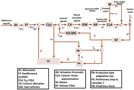
Figure 1.
System with L1 adaptive controller for dynamic positioning of caissons and Kalman filter.
2. Mathematical Representation of the Marine Structure
In the present paper, it is considered that the marine structure published in [23] is the object of study.
The dynamic model of the caisson, the object of study of this paper, is represented by the following equation [25]:
where are the position and the Euler angles of the caisson, M is the mass of the caisson, is the added mass at infinite frequency, K is the function of delay and fluid memory effects, C is the hydrostatic restoration coefficient, and are the external forces and moments, which can include the actuators and the waves. The caisson’s coordinate system is located in the center of gravity, and is considered inertial.
Due to the dynamics of this type of structure, which are of large dimensions, and the procedures that are currently used, the speeds at which these structures move are low. The following linear approximation of the cited structure is used in this work due to the low-speed operational conditions of this kind of structure [24]. As a result, the linear approximation used accurately represents the real dynamics of the system.
The terms in the above are as follows:
- is the state matrix.
- is the state vector. The coefficients of this vector correspond with the position and the Euler angles vector of the linearized model.
- is the input matrix.
- is the input vector. The coefficients of this vector correspond with the forces in , and the moment in .
- is the output matrix.
- is the output vector.
- is the feedforward matrix.
- is the identity matrix.
- is the zeros matrix.
Kalman Filter
A Kalman filter was implemented to filter the effects of disturbances, especially first-order waves. As a result, there were no adverse effects on the control system. The state vector was augmented to include the first-order waves so that the filter could estimate and filter them.
As indicated in [22], first-order wave effects are small zero-mean fluctuations that have to be filtered by the implemented Kalman filter for the system to work properly. The second-order wave effects are the so-called drift effects.
The following mathematical expressions were used to model first-order wave effects:
where is the damping, the gain is , is the wave intensity, is the wave dominant frequency, w is the Gaussian white noise, the state vector is , and the input vector is .
The second-order wave effects are represented by [22,26]:
where , , and are white noise vectors.
The model with augmented states corresponds to
with
where represents the inputs of the caisson, is the wave input vector, is the KF output vector, is the noise caused by the sensors (this effect is modeled with Gaussian white noise), and are the state space matrices of the waves, is the damping, the gain is , is the wave intensity, is the wave dominant frequency, and is the process noise (also modeled with Gaussian white noise).
The algorithm used in the implementation of a KF, as indicated in [20,21,22], can be seen in Figure 2.
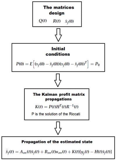
Figure 2.
Algorithm used in the implementation of a KF.
The Kalman filter has two tuning matrices, Q and R, i.e., the covariance of the states and the covariance of the noise, respectively. These matrices must be properly tuned for the correct operation of the filter and the system control. See details on the tuning [20,21,22].
- .
- .
where , , , , , and are the coefficients of the tuning matrix R, and , , , , , and are the coefficients of the tuning matrix Q.
3. L1 Adaptive Control
The application and implementation of an L1 adaptive control has been proposed. For this purpose, the adaptive control approach described in [27,28] was employed, in combination with a linear quadratic Gaussian (LQG) controller. It was implemented following the structure described in [18], which utilizes this system for the control of a nuclear power plant.
With this combination of control systems, the control loop is decoupled from the adaptation loop. This decoupling has extraordinarily positive effects on control, resulting in increased robustness by quickly rejecting and compensating for disturbances and deviations without losing effectiveness. Starting from the linear approximations of Model Equations (2) and (3), the corresponding terms for disturbances were added to the mathematical representation:
where represents sensor noise, is the discrepancy between the actual dynamics of the system and the mathematical representation applied to model it, denotes disturbances related to second-order wave effects, and represents the output of the model with the corresponding disturbances.
where represents the nominal control signals and represents the adaptive control. State Equation (3) can be expressed as follows:
where is the closed-loop system matrix, is the control feedback gain, is the input matrix, represents the disturbance, and is the input gain matrix of the system, which indicates the cross-coupling between different inputs.
The control consists of two different parts. Firstly, the control corresponds to the linear quadratic Gaussian controller, and secondly, the control corresponds to the adaptive control. The control scheme can be observed in Figure 1. Furthermore, the adaptive control adapts the control based on the projections of disturbances, which in turn were calculated using the prediction of future states of the caisson. The prediction block (adaptive control predictor) in Figure 1 performs the prediction of states:
where is the estimated state vector of the adaptation part, is the output vector, is the input matrix, is the estimated disturbance, and is the input gain matrix of the system, which indicates the cross-coupling between different inputs. Once the states are estimated, subtraction is performed with filtered states, resulting in the prediction error, denoted as .
The projection of disturbances is performed according to [18,28,29] as follows:
The projection operator in the previous equation is defined as follows [30]:
where represents the gradient of the convex function . This is defined as
where is the norm limit and is the tolerance in the projection, and is the solution of the algebraic Lyapunov equation. Finally, is the adaptation gain in Equation (3). As soon as the disturbances have been estimated, a preliminary step is taken to calculate the intermediate variable :
where .
Therefore, the adaptive control law has the following structure:
where
corresponds to the value of the feedforward filter (feedforward pre-filter) in the scheme shown in Figure 1. The feedforward filter is established so that the total system has the appropriate conditions for its control with the decoupling of the signals.
is one of the tuning variables, along with , which was chosen as an integrator.
4. Simulation Results
The simulations carried out in this section were performed to verify the behavior of the implemented L1 adaptive controller in the dynamic positioning system shown in Figure 1. All simulations are related to the caisson. They were conducted in the Matlab-Simulink environment with a time step of 0.1 s. In the simulation, the reference vector was set to Ref(t) = [5 m, 4 m, 0.175 rad]. The Kalman filter matrices were adjusted using
The LQR tuning matrices are adjusted as follows:
- ]
- ]
The tuning parameters of the L1 adaptive controller, , , and , are presented below in Table 1. The values of the control parameters and the Kalman filter were selected empirically.

Table 1.
Tuning parameters of the L1 adaptive control.
The wave parameters for all simulations are , , and , corresponding to an wave height. Please refer to Figure 3 and Figure 4 for visualization.
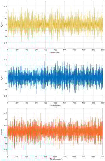
Figure 3.
Results of the system with L1 adaptive controller and waves. Effects of first-order waves applied to the caisson.
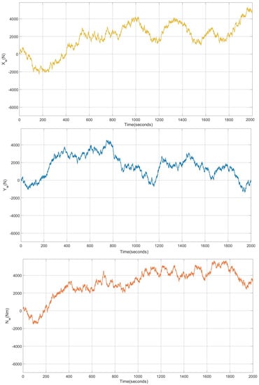
Figure 4.
Results of the system with L1 adaptive controller in the presence of waves. Forces and moments from second-order wave effects applied to the caisson.
The control system includes the L1 adaptive controller, composed of the LQG action combined with the adaptive control, which is able to compensate for the effects of second-order waves. Moreover, it performs the dynamic positioning properly, as can be seen in Figure 5, Figure 6, Figure 7 and Figure 8; the system presents a negligible steady-state error and remains stable during the whole simulation time. These results confirm the correct operation of the proposed controller.
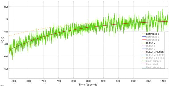
Figure 5.
Results of the system with disturbances and L1 adaptive control; position in x with zoom.
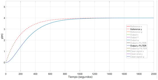
Figure 6.
Results of the system with disturbances and L1 adaptive control; position in y.
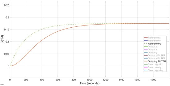
Figure 7.
Results of the system with disturbances and L1 adaptive control; heading position ().
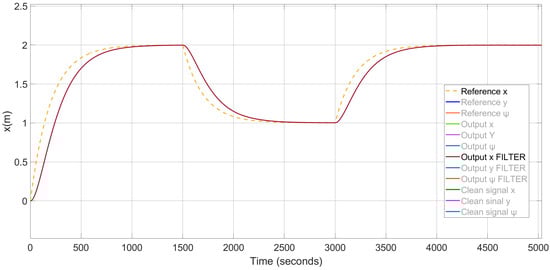
Figure 8.
Results of the system with disturbances and L1 adaptive control; position in x with squared reference signal.
In addition, the implemented Kalman filter effectively filters out first-order wave effects, and the adaptive controller predictions and projections provide accurate estimates of these effects.
The control system generates control signals without large oscillations, as seen in Figure 9. In addition, these control signals have low values with respect to the maximum values that can take. Finally, it should be noted that there are no oscillations or large changes in the tension of the lines, as shown in Figure 10 and Figure 11, which ensures that the system operates under safe conditions that will contribute to extend the lifetime of the actuators and improve the overall safety of the system.
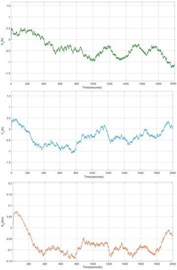
Figure 9.
Results of the system with disturbances and L1 adaptive control; control signals calculated by the controller.
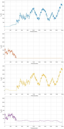
Figure 10.
Results of the system with disturbances and L1 adaptive control; stresses in lines 1 to 4.
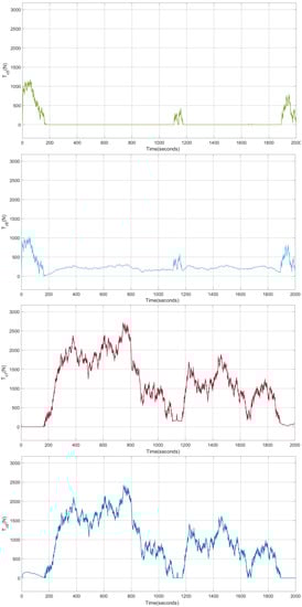
Figure 11.
Results of the system with disturbances and L1 adaptive control; stresses in lines 5 to 8.
Comparative Analysis of Controller Performance
The validity of the proposed controller has been previously exposed, and it was possible to see that it was able to position the structure as desired and that the control signals were acceptable. However, this is not enough to determine its advantages and disadvantages over other control methods and to establish its preferred application. As a result, a comparison of the results of the system with different controllers was carried out. The applied controllers are as follows:
- Double loop with a first-order filter (DLFPO). In this controller, two control loops are implemented: in the first one, an integral action is set to compensate for the effects of second-order waves, in the second loop, a feedforward network is implemented. For wave filtering, a first-order filter is implemented. For more information see [24].
- Double loop with linear quadratic Gaussian (DLLQG). Two control loops are established: in the first one, a proportional and integral action is implemented, and in the second loop, there is a LQG controller. A Kalman filter is used for filtering. For more information, see [24].
- GSMPC. In this controller, a double loop is implemented with an integral term in the first loop and an MPC controller that switches depending on the draught. A Kalman filter is implemented for wave filtering.
- L1 adaptive controller, i.e., the proposed controller in this paper. For more information, see Section 3.
For the comparative study, the systems were each simulated under the same environmental conditions. In this way, the perturbations corresponding to the waves were applied in the same conditions to all the systems with different controllers. These waves are m and the wave parameters for all the simulations are , and . Similarly, for all simulations, the reference vector was set to Ref(t) = [5 m, 4 m, 0.175 rad].
In order to determine which of these controllers generates a better global behavior of the system, and to observe the improvements between the implemented controllers, certain parameters were taken into account that are considered of vital importance. These are the following:
- Maximum control signal value, .
- Minimum control signal value, .
- Mean error in the last 20 measured values.
- L2 norm of the input, “”.
The maximum and minimum values of the control signal are important indicators as they determine the actuator forces or tensions in the system. Another important indicator is the average error over the last 20 values to establish the steady-state error in the positioning of the structure. It should be noted that the final values of positioning and control signals are not enough to determine the strengths or weaknesses of a control system. Other relevant factors include the form and variation in the control signals throughout the course of the process. It is noteworthy that the changes in the signals are smooth and do not have extreme values.
To evaluate the smoothness of the control signals, the L2 norm of the input (“”) was used, as conducted in [18]. This norm is expressed by the following equation:
All the values of the parameters established for the comparison should be as small as possible. That is, the lower these values are, the better the overall performance of the implemented controller. If we compare the responses of the different controllers in the minimum and maximum control signal with the parameters indicated corresponding to the output variable x, output y, and output , as shown in Table 2, Table 3 and Table 4, the following can be observed:
Table 2.
Comparison of results between controllers in x.
Table 3.
Comparison of results between controllers in y.
Table 4.
Comparison of results between controllers in .
- In the DLFPO controller, the minimum and maximum control signals are completely saturated in terms of the maximum and minimum values they can take. It is not acceptable, even if the caisson is properly positioned.
- For the DLLQG controller, the maximum and minimum values of the control signal are low, which will generate lower tensions than in the previous case.
- For the GSMPC controller, the maximum and minimum values of the control signal are considerably lower than those corresponding to the DLFPO controller. However, when compared to the DLLQG values, the minimum value is slightly lower but the maximum value is threefold greater than that of the DLLQG.
- Finally, the maximum value of the control signals of the L1 adaptive controller is the lowest of all the controllers, resulting in a significant improvement with respect to the first DLFPO controller and a considerable reduction with respect to both the DLLQG and GSMPC controllers. As for the minimum value of the control signal, it is very close to the value of the GSMPC, which is the lowest of all.
Then, a comparison was made between the results of the different controllers to determine whether there was a steady-state error and whether the control performed smoothly. For this purpose, the mean value of the last 20 positioning error data and the value of defined in the Equation (38) were compared. The results are presented in Table 5, Table 6 and Table 7. It can be seen that the only deviation that was significant is the one corresponding to the DLFPO controller in the y position, which deviated, on average, by about 2 cm. The rest of the position errors in the x position, y position, and position were negligible, so it can be considered that there was no steady-state error.
Table 5.
Comparative results among controllers in x.
Table 6.
Comparative results among controllers in y.
Table 7.
Comparative results among controllers in .
Furthermore, concerning the parameter indicating the control smoothness, the value corresponding to the DLFPO controller stands out logically as being significantly higher than the others. After this, the following controller with lower values is the GSMPC. Finally, it should be noted that both the DLLQG controller and the L1 adaptive controller have low values for , which indicates that the changes in the control signals were smooth.
The L1 adaptive controller and the DLLQG controller correctly positioned the caisson. There were no steady-state errors or process oscillations that could be considered significant. The maximum and minimum values of the control signals are low and the control is smooth, according to the results for . For all the abovementioned, it was determined that there was a significant improvement with this controller when compared to the results provided by the rest of the controllers. To complete this investigation, a Monte Carlo study of 200 realizations was carried out for the dynamic position of the drawer in the and positions of the DLLQG, L1 adaptive, and DLFPO controllers. The response of the DLFPO controller, which can be observed in Figure 12, exhibited a large dispersion compared to the response of the DLLQG controller in Figure 13 and that of the L1 adaptive controller in Figure 14. Finally, it was observed how the responses of the DLLQG and adaptive L1 controllers were precise and accurate. Higher precision and accuracy was observed in the L1 adaptive controller, as the points are more concentrated and nearer to the target.
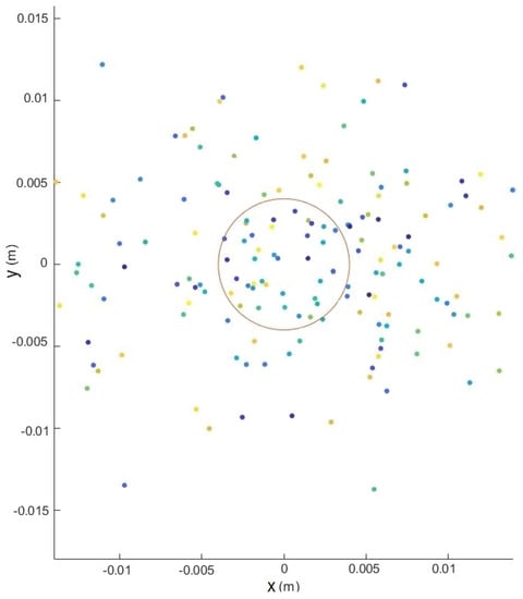
Figure 12.
System with DLFPO controller. Monte Carlo study of 200 realizations.
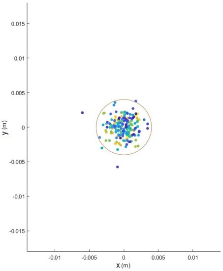
Figure 13.
System with DLLQG controller. Monte Carlo study of 200 realizations.
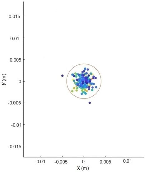
Figure 14.
System with L1 adaptive controller. Monte Carlo study of 200 realizations.
5. Conclusions
In this paper, the application of the L1 adaptive control technique for the dynamic positioning of marine structures was proposed. Several simulations of the proposed controller and other controllers, including LQG and MPC, were carried out. The application of the proposed controller shows that it is able to correctly position the caisson, compensating for the second-order effects of the waves and performing correct filtering of the disturbances corresponding to the first-order wave effects. The control signals do not present oscillations or saturations, which inherently results in an increase in the strength of the system as far as the safety of the operations is concerned. Monte Carlo studies were carried out to evaluate the precision and accuracy of the application of the different control techniques. It can be concluded that the proposed controller results in higher precision and accuracy than the other controllers. A fundamental consideration in the control systems is the magnitude and oscillations in the control signals that directly result in actuator tensions. The control signals were compared by employing statistical parameters and characteristic parameters. The L1 adaptive controller generates, in global terms, control signals of lower absolute value than the other controllers. This is a significant contribution concerning other controllers, since lower control signals will generate lower tensions in the lines. As a result, the equipment and actuators involved in the operations could be downsized. Another effect of the decrease in line tensions is the increase in the life of the equipment involved in the operations, as they have to work in less demanding conditions. It can be concluded that the application of the proposed L1 adaptive controller is a significant advancement in this area.
Author Contributions
Conceptualization, V.B. and J.J.S.; Methodology, V.B. and J.J.S.; Software, J.J.S. and E.R.H.; Validation, V.B. and J.J.S.; Formal Analysis, E.R.H. and J.R.L.; Investigation, V.B. and J.J.S. Resources, F.J.V., E.R.H. and J.R.L.; Data Curation, E.R.H. and J.R.L.; Writing—Original Draft Preparation, J.J.S.; Writing—Review and Editing, E.R.H. and J.R.L.; Visualization, V.B. and F.J.V.; Supervision, V.B., E.R.H. and J.R.L.; Project Administration, F.J.V. and E.R.H.; Funding Acquisition, F.J.V., E.R.H. and J.R.L. All authors have read and agreed to the published version of the manuscript.
Funding
This work was partially supported through the project TED2021-132158B-I00 “Evolutionary Monitoring with Unmanned Underwater Vehicles for the Maintenance of the bottom and Anchorages of Offshore Wind Farms” funded by MCIN/AEI/10.13039/501100011033, by the European Union—Next Generation, and through the project “Control of Unmanned Underwater Vehicles for Supervision of Structures for Anchored Maritime Works”. Funding was also received from the project “Advanced and Intelligent Controllers 3D Supervision” funded by the Ministry Of Universities, Equality, Culture and Sport of The Government of Cantabria.
Institutional Review Board Statement
Not applicable.
Informed Consent Statement
Not applicable.
Data Availability Statement
Data are available under request.
Conflicts of Interest
The authors declare no conflict of interest.
Abbreviations
The following abbreviations are used in this manuscript:
| DP | Dynamic positioning |
| KF | Kalman filter |
| LQG | Linear quadratic Gaussian control |
| LQR | Linear quadratic regulator |
| MPC | Model predictive control |
| UKF | Unscented Kalman filter |
References
- Gerwick, C. Construction of Marine and Offshore Structures, 3rd ed.; CRC: Boca Raton, FL, USA, 2007. [Google Scholar]
- Faltinsen, O. Hydrodynamic of High-Speed Marine Vehicles; Cambridge University Press: Cambridge, UK, 2005. [Google Scholar]
- Burgos Teruel, M. Guía Buenas Prácticas Para la Ejecución de Obras Marítimas; Puertos del Estado: Madrid, Spain, 2008. [Google Scholar]
- Fossen, T. Marine Control Systems: Guidance, Navigation and Control of Ships, Rigs and Underwater Vehicles; Marine Cybernetics: Tiller, Norway, 2002. [Google Scholar]
- Grinyak, V.M.; Pashin, S.S. Control of the Vessel Course using of PID-Regulator under Parametric Uncertainty. In Proceedings of the IOP Conference Series. Earth and Environmental Science, Bogor, Indonesia, 16–18 September 2020; Volume 459, p. 22011. [Google Scholar]
- Ogata, K. Ingenieria de Control Moderna, 5th ed.; Pearson Educacion: Naucalpan de Juárez, Mexico, 2010. [Google Scholar]
- Carlucho, I.; Menna, B.; De Paula, M.; Acosta, G.G. Comparison of a PID controller versus a LQG controller for an autonomous underwater vehicle. In Proceedings of the 3rd IEEE/OES South American International Symposium on Oceanic Engineering (SAISOE), Buenos Aires, Argentina, 15–17 June 2016; pp. 1–6. [Google Scholar]
- Wadoo, S.A.; Sapkota, S.; Chagachagere, K. Optimal control of an autonomous underwater vehicle. In Proceedings of the IEEE Long Island Systems, Applications and Technology Conference (LISAT), Old Westbury, NY, USA, 5 May 2012; pp. 1–6. [Google Scholar]
- Noh, M.M.; Arshad, M.R.; Mokhtar, R.M. Depth and pitch control of USM underwater glider: Performance comparison PID vs. LQR. Indian J. Mar. Sci. 2011, 40, 200–206. [Google Scholar]
- Grune, L.; Pannek, J. Nonlinear Model Predictive Control: Theory and Algorithms; Springer International Publishing AG: Cham, Switzerland, 2016. [Google Scholar]
- Fannemel, Å.V. Dynamic Positioning by Nonlinear Model Predictive Control. Master’s Thesis, Institutt for Teknisk Kybernetikk, Trondheim, Norway, 2008. [Google Scholar]
- Arab-Alibeik, H.; Setayeshi, S. Adaptive control of a PWR core power using neural networks. Ann. Nucl. Energy 2005, 32, 588–605. [Google Scholar] [CrossRef]
- Mousakazemi, S.M.H.; Ayoobian, N. Robust tuned PID controller with PSO based on two-point kinetic model and adaptive disturbance rejection for a PWR-type reactor. Prog. Nucl. Energy 2019, 111, 183–194. [Google Scholar] [CrossRef]
- Xia, G.; Xue, J.; Sun, C.; Zhao, B. Backstepping Control Using Barrier Lyapunov Function for Dynamic Positioning Control System with Passive Observer. Math. Probl. Eng. 2019, 2019, 8709369. [Google Scholar] [CrossRef]
- Xu, L.; Liu, Z. Design of fuzzy PID controller for ship dynamic positioning. In Proceedings of the 2016 Chinese Control and Decision Conference (CCDC), Yinchuan, China, 28–30 May 2016; pp. 3130–3135. [Google Scholar]
- Xia, G.; Xue, J.; Jiao, J. Dynamic Positioning Control System with Input Time-Delay Using Fuzzy Approximation Approach. Int. J. Fuzzy Syst. 2018, 20, 630–639. [Google Scholar] [CrossRef]
- Zhao, D.; Gao, S.; Spurgeon, S.K.; Reichhartinger, M. Adaptive Sliding Mode Dynamic Positioning Control for a Semi-Submersible Offshore Platform. In Proceedings of the 18th European Control Conference (ECC), Piscataway, NJ, USA, 11–14 July 2019; pp. 3103–3108. [Google Scholar]
- Vajpayee, V.; Becerra, V.; Bausch, N.; Deng, J.; Shimjith, S.R.; Arul, A.J. L1-Adaptive Robust Control Design for a Pressurized Water-Type Nuclear Power Plant. IEEE Trans. Nucl. Sci. 2021, 68, 1381–1398. [Google Scholar] [CrossRef]
- Kalman, R.E. A New Approach to Linear Filtering and Prediction Problems. Trans. Asme-J. Basic Eng. 1960, 82, 35–45. [Google Scholar] [CrossRef]
- Grewal, M.S. Kalman Filtering: Theory and Practice Using MATLAB, 3rd ed.; John Wiley and Sons: Hoboken, NJ, USA, 2008. [Google Scholar]
- Fossen, T.I.; Perez, T. Kalman filtering for positioning and heading control of ships and offshore rigs. IEEE Control. Syst. Mag. 2009, 29, 32–46. [Google Scholar]
- Fossen, T.I. Handbook of Marine Craft Hydrodynamics and Motion Control; John Wiley and Sons, Ltd.: Hoboken, NJ, USA, 2011; Available online: https://onlinelibrary.wiley.com/doi/pdf/10.1002/9781119994138.fmatter (accessed on 13 August 2023).
- Revestido Herrero, E.; Llata, J.R.; Gonzalez-Sarabia, E.; Velasco, F.J.; Sainz, J.J.; Rodriguez-Luis, A.; Fernandez-Ruano, S.; Guanche, R. Dynamic positioning of floating caissons based on the UKF filter under external perturbances induced by waves. Ocean. Eng. 2021, 235, 109055. [Google Scholar] [CrossRef]
- Sainz, J.J.; Revestido Herrero, E.; Llata, J.R.; Gonzalez-Sarabia, E.; Velasco, F.J.; Rodriguez-Luis, A.; Fernandez-Ruano, S.; Guanche, R. LQG Control for Dynamic Positioning of Floating Caissons Based on the Kalman Filter. Sensors 2021, 21, 6496. [Google Scholar] [CrossRef] [PubMed]
- Armesto, J.A.; Guanche, R.; Jesus, F.d.; Iturrioz, A.; Losada, I.J. Comparative analysis of the methods to compute the radiation term in Cummins’ equation. J. Ocean. Eng. Mar. Energy 2015, 1, 377–393. [Google Scholar] [CrossRef]
- Pérez, T. Ship Motion Control: Course Keeping and Roll Stabilisation Using Rudder and Fins; Springer: London, UK, 2005. [Google Scholar]
- Cao, C.; Hovakimyan, N. L1 adaptive controller for systems with unknown time-varying parameters and disturbances in the presence of non-zero trajectory initialization error. Int. J. Control 2008, 81, 1147–1161. [Google Scholar] [CrossRef]
- Hovakimyan, N.; Cao, C. L1 Adaptive Control Theory: Guaranteed Robustness with Fast Adaptation; Society for Industrial and Applied Mathematics: Philadelphia, PA, USA, 2010. [Google Scholar]
- Cao, C.; Hovakimyan, N. Design and analysis of a novel L1 adaptive control architecture with guaranteed transient performance. IEEE Trans. Autom. Control 2008, 53, 586–591. [Google Scholar] [CrossRef]
- Pomet, J.; Praly, L. Adaptive nonlinear regulation: Estimation from the Lyapunov equation. IEEE Trans. Autom. Control 1992, 37, 729–740. [Google Scholar] [CrossRef]
Disclaimer/Publisher’s Note: The statements, opinions and data contained in all publications are solely those of the individual author(s) and contributor(s) and not of MDPI and/or the editor(s). MDPI and/or the editor(s) disclaim responsibility for any injury to people or property resulting from any ideas, methods, instructions or products referred to in the content. |
© 2023 by the authors. Licensee MDPI, Basel, Switzerland. This article is an open access article distributed under the terms and conditions of the Creative Commons Attribution (CC BY) license (https://creativecommons.org/licenses/by/4.0/).