Abstract
This study aimed to improve the performance of a wastewater treatment plant (WWTP) simulated with Benchmark Model No. 2 (BSM2). To achieve this objective, three control strategies were implemented and tested. The first control strategy aimed to maintain the concentration of nitrate and nitrite nitrogen (SNO) by controlling the external carbon flowrate (strategy A1), and the second control strategy aimed to maintain the ammonia and ammonium nitrogen (SNH) at a desired level with the use of a cascade controller (strategy A2). The third strategy was applied to control the total suspended solids (TSS) (strategy A3). Combinations of these strategies were considered (B1, B2, and B3 strategies), as well as the use of all three together (strategy C1). The control strategies presented in this paper were compared to the default control strategy of BSM2 to validate and identify the one that provided the best performance. The results revealed that the B1 strategy was the most environmentally friendly, while C1 obtained the highest overall performance. Several Monte Carlo simulations were performed for the validated control strategies, to identify the optimal setpoint values. For the C1 strategy, a second method of optimization regarding polynomial interpolation was considered. The applied optimization methods provided the optimal reference values for the PI (proportional integral) controllers.
MSC:
93B52
1. Introduction
Wastewater represents a threat to human health and well-being [1], it can also affect the environment through being directly discharged into different surface water bodies [2]. Nutrient-rich wastewater can lead to eutrophication [3], which affects both freshwater and seawater [4]. Other pollutants found in the composition of wastewater and contaminated water bodies represent real environmental hazards, such as petroleum products [5] and heavy metals [6]. Wastewater treatment plants (WWTP) with activated sludge are used worldwide to prevent such environmental hazards from happening. Recent studies, such as [7], indicated that the sludge obtained from WWTPs can be successfully used in agriculture, the only disadvantage being the need for continuous monitoring of the soil and sludge composition, to avoid heavy metal contamination. The study in [8] indicated that, in the case of water body contamination with wastewater, regulated monitoring of the physicochemical quality indices is important to determine the level of pollution.
To increase the performance of a WWTP, various control strategies need to be tested and evaluated, to select the one that provides the best results. Testing such control strategies on pilot WWTPs is not ideal, taking into account the possible environmental risks and the additional operational costs. A solution to this problem is the use of benchmark models, such as Benchmark Simulation Model No. 2 (BSM2) [9]. This model is widely used in the field of wastewater treatment, being highly appreciated and used by the scientific community.
BSM2 promotes the idea of implementing and testing user-made control strategies. In the literature, there are various examples of configurations that aim to improve the performance of this simulated WWTP. Such control strategies can be found by consulting the specialized literature in the field.
In the study in [10], a fuzzy controller was used to reduce nitrous oxide emissions by minimizing oxygen levels. Another study [11] proposed the use of a fuzzy logic controller, to avoid violation of the BSM2 effluent quality limits for nitrogen and ammonia concentrations.
In the paper in [12], the default control strategy of BSM2 was optimized using the iterative relaxation method. The use of such iterative methods has proven to be useful when the known PI controller’s setpoint value must be fine-tuned.
In the study in [13], two hierarchical control loops were proposed, one with a combination of proportional integral-model predictive control (PI-MPC) controllers for the lower level of control, and an MPC-Fuzzy combination for the higher level, with the purpose of enhancing the performance and reducing the operational cost of the plant.
The influent represents the wastewater that enters the WWTP. The influent can be described by its flow rate and load at the entrance to the WWTP. Usually, these influent characteristics are hard to predict, which is the reason why most WWTPs are designed with risk prevention control strategies, usually with bypass systems that are used in case the influent flow rate and load surpass the treatment capacity of the plant. The study in [14] proposed an extension for BSM2 including a sewer network. By implementing a sewer network model in BSM2, multiple options for generating the influent for the simulated WWTP become available; thus, urban WWTP operators can test different realistic scenarios regarding the flow rate and load of the influent.
In the study in [15], a control strategy based on fuzzy logic was implemented in a modified version of BSM2, called BSM2-PSFe [16], which is capable of describing the compound transformations and connections between phosphorus, sulfur, and iron cycles. Different combinations of PI and fuzzy logic controllers were able to successfully improve the effluent quality and the operational cost of the simulated WWTP. The efficiency index proposed in the previously mentioned work is computed as the ratio between the removed nitrogen during denitrification and the energy required for nitrogen removal.
The overall performance of WWTP can be improved by applying simple control loops governed by PID (proportional integral derivative) controllers. In BSM2, the most important control parameter in the aerated section of the bioreactor is dissolved oxygen. Manipulation of this parameter was proposed in [17], where a PID control loop was proposed to minimize the difference between the efficiency index and the desired value.
The optimization of the nitrification and denitrification processes is crucial in wastewater treatment. By conducting an optimized treatment process, the best results are usually obtained. The objective of achieving an optimized wastewater treatment process is discussed in the study in [18], where different fuzzy controllers and MPC were used to create control strategies that aimed to increase the performance of the nitrification and denitrification processes of the bioreactor. The study also proposed a method for detecting the best control strategy, using artificial neural networks to analyze effluent violations.
One of the key elements in optimizing wastewater treatment processes using PI controllers is to find the optimal setpoint value for such controllers. There are different ways to identify or compute the setpoint of the PI controller proposed in the specialized literature. The setpoint of the PI controller is usually considered constant, but it can also be dynamically computed, especially in the case of more complex control strategies. The study in [19] proposed a method of computing a dynamic reference value for a PI controller by predicting the aeration energy consumption with an artificial neural network.
The operation of WWTPs is marked by uncertainty regarding the influent flow rate and component load. Often, WWTP operators are defenseless against different scenarios where both the capacity and the treatment capability of the plant are passed, caused by an unexpected event such as torrential rain. In such situations, the operators are caught off guard and often a large portion of the influent must be bypassed, being discharged directly into the collecting body of water. In reality, every violation of effluent quality parameters may be fined by the responsible authorities, thus affecting the cost-efficiency of the plant. The effluent limit violations of different wastewater quality parameters are also included in BSM2; in the specialized literature, they are usually considered as a secondary performance criterion to evaluate the user-made control strategies. The work in [20] proposed a solution to such situations, using artificial neural networks to detect possible concentration violations of nitrogen and ammonia from the effluent. A similar idea was proposed in the paper [21], where the effluent concentrations were predicted using an alarm generation system based on artificial neural networks.
In the paper in [22], Monte Carlo simulations were performed with the open-loop and closed-loop versions of BSM2. The study proposed two control strategies for the bioreactor. The first strategy uses an oxygen controller, while the second strategy uses a cascade controller, where an ammonium controller regulates the setpoint for the oxygen controller. Monte Carlo simulations were used to generate different values for different plant parameters, such as the internal recirculation flow rate, bioreactor tank volumes, oxygen coefficient ratio, and setpoint of DO (dissolved oxygen) for one of the controllers. The parameters that had less influence over the evaluation criteria were identified and discarded via sensitivity analysis. Moreover, different plant parameters will provide different outcomes in terms of performance and cost efficiency. Thus, various scenarios and plant configurations were tested. By applying this uncertainty analysis method, the optimal version of the control strategies was identified.
In the study in [23], a global sensitivity analysis was performed by combining Monte Carlo simulations with standardized regression coefficients, which were applied to classify parameters by their influence over the BSM2 influent. A similar approach was utilized in the paper in [24], where instead of Monte Carlo simulations, a global sensitivity analysis was performed using polynomial chaos expansion, Gaussian process regression, and artificial neural networks.
The purpose of the present study was to obtain an enhanced performance for a simulated WWTP through implementing, testing, optimizing, and evaluating three control strategies within the framework of BSM2. All control strategies were implemented individually and in a combined manner, and this comparative method was chosen for strategy validation.
2. Benchmark Simulation Model No. 2
BSM2 was used in this study, and this model represents an important software tool for evaluating the performance of a simulated WWTP with activated sludge. The model was developed by the International Water Association (IWA) Task Group on Benchmarking of Control Strategies for WWTPs [9]. BSM2 is capable of simulating a WWTP with two stages of treatment. The first stage represents wastewater treatment, focused on removing the organic substances and nutrients (nitrogen), to obtain a high-quality effluent. Activated Sludge Model No. 1 (ASM1) [25] was included in the framework of BSM2 to describe the biological and chemical processes that occur in the bioreactor. This makes BSM2 capable of simulating important wastewater treatment processes such as nitrification and denitrification.
In the case of BSM2, the second treatment stage refers to sludge treatment, recirculation, and removal.
The sludge forms through the sedimentation of suspended solids in the primary and secondary clarifier, being further distributed across different treatment installations. The first sludge treatment installation is the thickener. In reality, at this point, the sludge is compressed using various mechanical processes (gravitational sedimentation, rotary drum thickeners, etc.) [26]. This is a process in which the volume of the sludge is reduced and it is prepared to be used in the next treatment installations.
In the next step, the sludge is pumped into the anaerobic digester. Anaerobic Digestion Model No. 1 (ADM1) [27,28] was also implemented within the framework of BSM2, to describe the biochemical and physicochemical reactions that occur inside the anaerobic digestor. One key element of this process is the production of biogas, which is further used to sustain the energetic autonomy of the plant.
Lastly, the sludge is pumped into the dewatering unit, whose purpose is to remove any remaining water from the sludge. In reality, this process is carried out using various methods [29]: natural dewatering, drying bed, press filter, belt press filter, press filter with screw, rotary press, solid bowl centrifuge, electro-dewatering, liquid sludge, etc.
The active sludge is recirculated during the wastewater treatment stage to maintain a constant concentration in the bioreactor; in this way, the concentration of the microorganisms is maintained without being flushed out of the system, and thus the nitrification and denitrification processes are controlled.
The basic structure of BSM2 is presented in Figure 1 and includes the following treatment units:
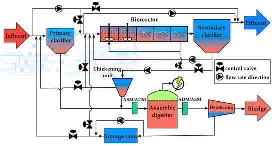
Figure 1.
Overview of BSM2 plant layout.
- Primary clarifier—based on the models developed by [30,31], which describe a biologically inert clarifier. Within this unit, the first separation of sludge and water takes place before the influent enters the bioreactor. The considered volume capacity for the clarifier is 900 m3;
- Activated sludge bioreactor for nitrogen removal, whose activity is described by the ASM1 model. The bioreactor consists of 5 compartments, with compartments 1–2 operating in anoxic conditions and compartments 3, 4, and 5 operating in aerobic conditions, where specific nitrification and denitrification processes occur. The volume considered for the bioreactor is 12,000 m3;
- Secondary clarifier—where excess activated sludge is separated from the water, based on the dynamic settling and thickening model developed by [32]. The volume capacity of this unit is 6000 m3. The model does not describe any biological processes.
- Sludge thickening station—capable of achieving a solid removal efficiency of 98% [33]. This unit is modeled as being biologically inert.
- Anaerobic digestion station (ADM1);
- Sludge drying station—the final stage before removing the sludge from the system, this unit is modeled as a biologically inert installation.
- Storage station—the physically-based model describes the process of collecting water obtained during the drying process. The station has a volume capacity of 160 m3.
A dynamic influent was considered for 609 days. The period between day 0 to day 245 represents the period of plant stabilization, while the period from day 245 to day 609 represents the observation time.
The performance evaluation of the implemented control strategies was conducted using BSM2′s evaluation tools, using mathematical equations that represent the quality of the influent—IQI (influent quality index), the effluent—EQI (effluent quality index), and the operational cost of the treatment plant—OCI (overall cost index), while taking into account only the observation period.
IQI is expressed in kg pollution unit/day, and it is used to indicate the pollution load of the influent. The difference between the IQI and EQI shows the treated pollution load using the simulated WWTP.
where tobs is the observation time, TSS (total suspended solids), COD (chemical oxygen demand), NKj (Kjeldahl nitrogen concentration), NO (nitrite and nitrate concentration), and BOD5 (biochemical oxygen demand), Bi represents the weighting factors, and Qi is the influent flow rate.
The EQI (measured in kg pollution unit/day) is the average value of the sum of the weighted effluent loads of the primary wastewater compounds that have a major influence on the quality of the receiving water, calculated over the observation period of one year (364 days). Additionally, when user-implemented control strategies are employed, the EQI can offer valuable insights into the impact of these strategies on the treatment performance of the plant.
EQI is computed using the following mathematical expression:
where Qe is the effluent flow rate.
The weighting factors for specific influent and effluent parameters have the following values: BTSS = 2, BCOD = 1, BNKJ = 30, BNO = 10, and BBOD5 = 2. The applied values indicate that NKJ has the strongest impact on IQI and EQI.
The purpose of the OCI can be interpreted in two ways. First, it serves to provide information regarding the operating costs of the entire plant. Second, it provides valuable insights into the energetic performance of the control strategies used. OCI analysis can provide a comprehensive understanding of the financial implications and efficiency of the control measures implemented within plant operations.
The simulated WWTP effluent is described by the following mathematical relation:
where Qsc,e is the overflow rate from the secondary clarifier and Qbypass is the bypassed flow rate of raw wastewater.
OCI is described using the following mathematical relation:
where AE is the energy consumed for aeration, PE is the energy consumed by the pumping system, SP is sludge production, EC is external carbon consumption, ME is mixing energy, METprod is the production of biogas, and HEnet is the energy consumed for heating.
During the performance analysis stage, the BSM2 model utilizes threshold values for the concentrations of key quality parameters in the effluent. These threshold values can be modified based on user preferences. In this case, the maximum allowable values used were the standard values specified in the BSM2 model, as presented in Table 1.

Table 1.
BSM2 limit values for effluent parameters.
The influent and effluent quality parameters are described in BSM2 by the ASM1 variables. The primary variables used by the model are soluble inert organic matter (SI), readily biodegradable substrate (SS), particulate inert organic matter (XI), slowly biodegradable substrate (XS), active heterotrophic biomass (XB,H), active autotrophic biomass (XB,A), particulate products arising from biomass decay (XP), oxygen (SO), nitrate and nitrite nitrogen (SNO), nitrogen ammonia and ammonium (SNH), soluble biodegradable organic nitrogen (SND), particulate biodegradable organic nitrogen (XND), and alkalinity (SALK). Other variables include time (days), influent/effluent flow rate (m3/days), and temperature (°C).
The effluent Ntot is computed with the following mathematical formula:
The effluent CODtot is computed with the following mathematical formula:
The effluent SNKj,e is computed with the following mathematical formula:
The effluent TSS is computed with the following mathematical formula:
The effluent BOD5 is computed with the following mathematical formula:
BSM2 introduces a basic control strategy that is depicted schematically in Figure 2 and hereinafter referred to in this article as DefCL. This strategy represents a starting point for new BSM2 users for how they can build and implement their custom control strategies.
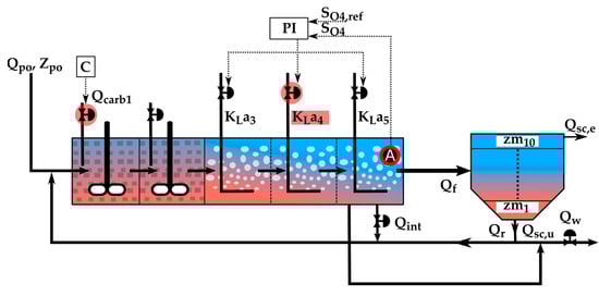
Figure 2.
DefCL control strategy.
The DefCL strategy comprises two control loops to optimize the nitrification and denitrification processes in the bioreactor. The first control loop aims to maintain the dissolved oxygen (DO) level in bioreactor tank no. 5 at a predefined value of 2 g (-COD)/m3. This is achieved by manipulating the oxygen transfer coefficient KLa4 in bioreactor tank no. 4 to ensure compliance with the following relationships:
where KLa3 is the oxygen transfer coefficient for tank no. 3 of the bioreactor, and KLa5 is the oxygen transfer coefficient for tank no. 5 of the bioreactor.
Within the DefCL strategy, the addition of carbon from external sources into the first tank of the anoxic zone in the bioreactor, at a constant flow rate of 2 m3/day (Qcrab1), is considered. The purpose of this action is to enhance the potential of the denitrification process. This is achieved through the manipulation of the actuator that controls the carbon flow rate, Qcarb1.
The results obtained with the DefCL strategy can be used as a reference for comparing the outcomes with other user-created control strategies.
Where Qpo represents the influent flow rate, Zpo is the influent concentrations, C means constant value, PI is the proportional integral controller, SO4,ref is the setpoint for the PI controller, SO4 is the dissolved oxygen (DO) value measured by a type A sensor, Qint is internal recycle flow rate, Qr is the external recycle flow rate, Qf is the flow rate of the water that exits the bioreactor towards the secondary clarifier, Qsc,u is the underflow rate of the secondary clarifier, Qsc,e is the overflow rate from the secondary clarifier, Qw is the wastage flow rate, zm is equal to 1 m and represents the height of each of the 10 levels of the secondary clarifier.
In addition to the manipulable execution elements, the model also includes a PI-type controller and sensors classified into six categories, based on the measured parameters and response time (A, B0, B1, C0, C1, and D).
3. Implemented Control Strategies
In this study, the BSM2 model was employed. Three control strategies, presented for the first time in the study [34], were evaluated to identify the strategy that provided the best performance for further optimizations. The control strategies were tested in an individual (strategy A1, A2, A3), combined (strategy B1, B2, B3), and comprehensive manner (strategy C1). The strategies A1, A2, and A3 correspond with the WL-A2, WL-A4, and SL-A1 control strategies from the paper [34].
The purpose of this paper was to compare the results obtained with the proposed control strategies, to identify the best control strategy, and with an attempt to optimize the PI controllers’ reference values. A more detailed description of each control loop can be found in the paper in [34].
The first control strategy implemented, represented in Figure 3 and hereafter referred to as A1, includes the following control elements: a PI controller, a B0-type sensor, and an actuator (valve). The B0 type is used to measure the concentration of SNO from the second anoxic tank of the bioreactor. The PI controller computes the optimal value of the external carbon flow rate (Qcarb1) based on the measured value of SNO and the setpoint value for external carbon addition (Qcarb,ref). The considered value for Qcarb,ref is 1 m3/day. The objective of this control strategy is to support the DefCL, by converting the constant flow rate of external carbon addition into a closed loop. In this way, it was considered that the denitrification process would be optimized, resulting in a better overall performance.
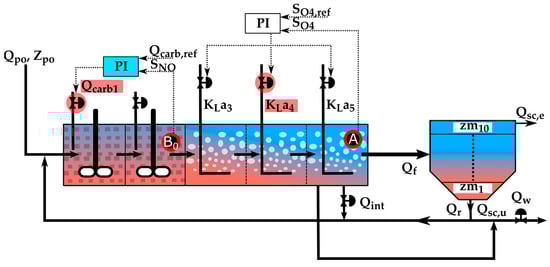
Figure 3.
A1 control strategy.
The second control strategy, hereafter referred to as A2 and presented in Figure 4, acts as a support for the DefCL by involving a cascade controller (PI-PI), which involves a higher-level PI controller. The higher-level control loop contains a PI controller and an A-type sensor. The sensor is used to measure the SNH from the fifth aerated tank of the bioreactor. The purpose of the higher-level controller is to compute a dynamic setpoint for the second PI controller, based on the measured values of SNH and the reference value of 1 g N/m3 represented by SNH,ref.
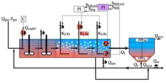
Figure 4.
A2 control strategy.
The third control strategy, hereafter referred to as A3 presented in Figure 5, does not have a direct connection with DefCL. The A3 components include a PI controller, an A-type sensor, and an actuator. The sensor has the purpose of measuring the TSS concentration in the fifth tank of the biological reactor. The measured information is used by the PI alongside the considered reference value of 4000 g SS/m3 (TSSref) to compute an optimal value for Qw.
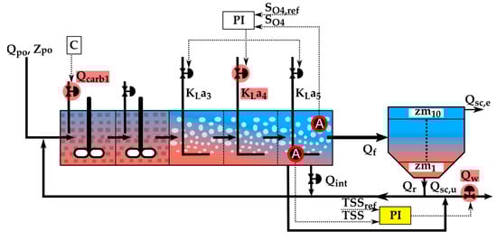
Figure 5.
A3 control strategy.
Strategy B1, presented in Figure 6a, represents a combination of strategy A1 and A2. The strategy involves a newly implemented control loop and a cascade controller to maintain the SNO and SNH concentration in the first and the last tank of the bioreactor at a desired value.
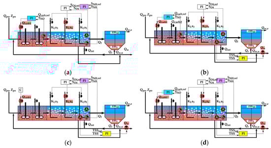
Figure 6.
Combined control strategies: B1 (a), B2 (b), B3 (c), and C1 (d).
Strategy B2, presented in Figure 6b, is formed by the simultaneous implementation of strategies A1 and A3. Thus, two control loops were considered: one designed to maintain the SNO at a desired value in the first anoxic tank, and the other, with the same purpose, for the TSS from the fifth tank of the biological reactor.
Strategy B3, presented in Figure 6c consists of strategies A2 and A3, which were implemented together, to control the concentration of SNH and TSS in the last aerated tank of the bioreactor.
The most complex strategy used in this paper is strategy C1, presented in Figure 6d. This strategy represents the simultaneous implementation of the A1, A2, and A3 strategies. The purpose of this strategy was to control the concentration of SNO in the first anoxic tank and the SNH and TSS in the last aerated tank.
4. Additional Evaluation Criterion
An overall performance criterion (OPC) was proposed to summarize the performance and the operational cost of the control strategies. The OEC takes into account the equal importance of the EQI and OCI for classifying the control strategies using their final results.
The OPC has the following mathematical formula:
where and represent the normalized values of and .
Taking into account that EQI and OCI reflect the real performance of the simulated WTTP, a secondary tiebreaker criterion was considered to identify the strategy that is the most environmentally friendly. Thus, an environmentally friendly criterion (EFC) was formulated as:
where , represent the normalized values for the violation time (VT) of all effluent quality parameters.
5. Evaluation of the Considered Control Strategies
The intermediate results represent the performance of the control strategies regarding their environmental and legal impact and are presented in Figure 7. In practice, exceeding the limit values for all effluent quality parameters may result in penalties imposed on the operator of the WWTP. In the case of BSM2, this idea is not implemented but it is reflected by the EQI.
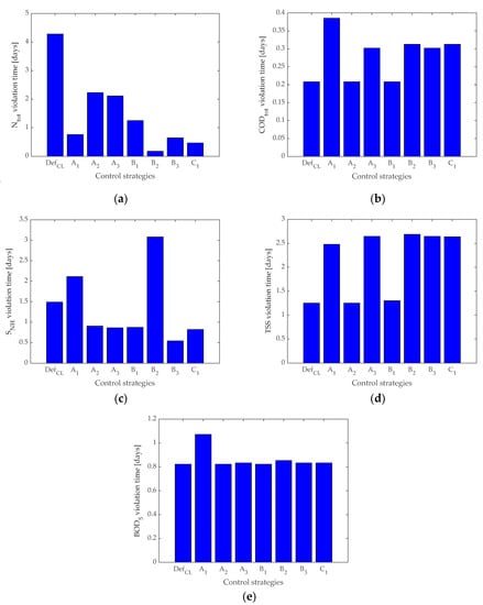
Figure 7.
Intermediate values were obtained for all control strategies representing Ntot, (a), CODtot, (b) SNH (c), TSS (d), and BOD5 (e).
We must take into account that the control strategy that obtained the shortest violation time for a specific effluent quality parameter represents the best performance regarding the environmental impact.
The violation time for Ntot is presented in Figure 7a. The shortest violation time was obtained by the B2 strategy (0.177 days), followed by C1 (0.468 days).
For CODtot, the intermediate results are presented in Figure 7b. Control strategies DefCL, A1, and B1, obtained the best performance, the recorded violation time for all three strategies was 0.283 days.
In the case of SNH, presented in Figure 7c, the shortest violation time was obtained with the B3 control strategy, representing 0.5417 days.
Figure 7d, presents the violation time for TSS. The best performance was obtained with the DefCL strategy, followed by the results obtained with the A2 and B1 strategies.
Finally, the results, presented in Figure 7e indicate that the shortest violation time for BOD5 was recorded with the DefCL, A2, and B1 control strategies.
All the results were compared regarding the DefCL control strategy as a reference point. The results shown in Figure 8 indicate that the strategy with the smallest negative impact on the environment was B1. The second place was taken by strategy A2. The other control strategies obtained performances that were above the reference.
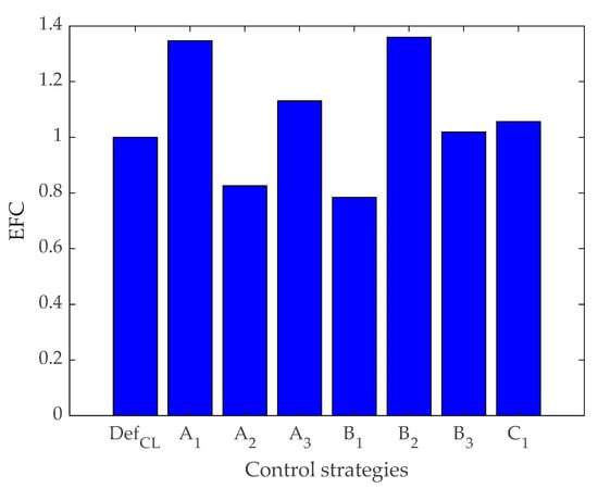
Figure 8.
EFC values.
The most important evaluation within BSM2 is represented by the EQI and OCI indexes. The overall performance of the plant can be approximated by consulting the values of these important evaluation factors.
The results regarding the EQI values, presented in Figure 9a, indicate that the best performance was obtained using the C1 strategy, recording 5.039433478034807 × 10³ kg poll. units/day. If we analyze the results presented in Figure 9b, we can observe that strategy C1 also obtained the best result compared to all other control strategies regarding the operational cost of the plant.
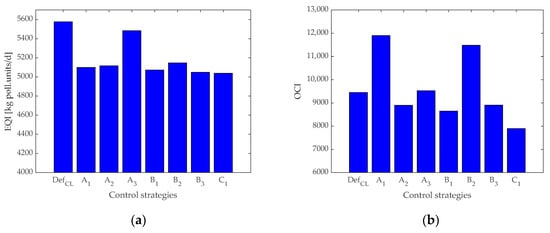
Figure 9.
Values were obtained with all control strategies for EQI (a); OCI (b).
The data presented in Figure 10 was used for strategy validation, regarding the effluent quality and the operational cost, which was obtained by applying Equation (12). The best results were obtained by using strategy C1 (0.869), the second place was taken by the B1 strategy with 0.912, and the third place was taken by strategy B3 with 0.923.
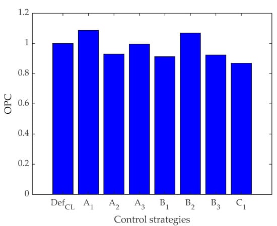
Figure 10.
Strategy validation data for OPC.
Monte Carlo simulations are used as part of uncertainty analysis, with the scope of exploring a wide range of possible input combinations by using random sampling from input parameter distributions. In our case, the considered input parameters that were randomized were the reference values for the PI controllers (Qcarb,ref, SNH,ref, and TSSref). To randomize the sampling from input parameter distributions, the following mathematical relation was formulated:
where Xn represents the parameter for which the random values are being generated. (X1 = Qcarb,ref, X2 = SNH,ref, X3 = TSSref) that follow a normal distribution N(μ, σ2) and are constrained within the range Z describing the range [minval, maxval]; μ is considered as the mean value of the considered parameter; σ is the standard deviation used in the normal distribution.
The algorithm used to generate the random numbers with a normal distribution follows the steps mentioned below:
Step 1: Generate a standard normal random variable Z ~ N(0, 1);
Step 2: Scale Z to fit within the desired range [minval, maxval];
Step 3: Ensure that X is truncated to be within the desired range [minval, maxval].
For each input parameter, the [minval, maxval] range condition was determined as the minimum and maximum detected value for nitrate and nitrite nitrogen, ammonia and ammonium nitrogen, during the simulation with DefCL. For TSSref, the generated data were truncated between 3997 and 4004 g SS/m3. The data regarding the considered range values are provided in Table 2.
Table 2.
Range values for Monte Carlo simulation input parameters.
For Qcarb,ref, since the BSM2 model does not provide any sensors to measure the added carbon in the bioreactor, the detected limit values for nitrate and nitrite nitrogen were considered.
The B1 and C1 strategies were selected to perform the Monte Carlo simulations. The objective was to identify the optimized reference values (Qcarb,ref, SNH, ref, and TSSref) for the PI controller. Since the PI controller’s reference points have a great impact on the outcome of the applied control strategies, different values provide different performances regarding the effluent quality and the operational cost.
For the B1 control strategy, 100 Monte Carlo simulations were performed, to record a better EFC performance, regarding the variance of Qcarb,ref, and SNH,ref reference values.
In the case of strategy B1, the generated and applied values for Qcarb,ref, are presented in Figure 11a. The data indicate that the lowest recorded value for Qcarb,ref was 0.01631 m3/day, while the highest was 3.286 m3/day. The mean value for the Qcarb,ref dataset was 1.273 m3/day, with a standard deviation of 0.6972 m3/day. Figure 11b shows the arranged data in the form of a histogram with seven categories. The category for values between 1 and 1.5 m3/day includes the most generated values (29 values), while the category for values in the 3–3.5 m3/day range includes just 1 value.
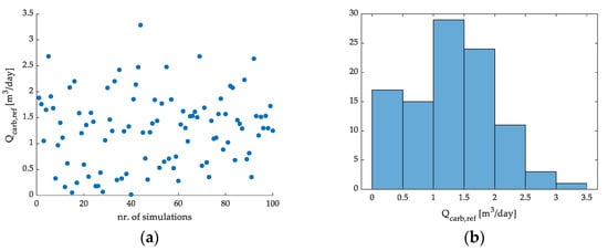
Figure 11.
Scatter plot of the generated and applied Qcarb,ref data for B1 strategy (a), and histogram of the data (b).
Figure 12a shows the generated and applied values for SNH,ref. The presented data show that the lowest recorded value for SNH,ref was 0.1125 g N/m3 and the maximum value was 3.567 g N/m3, while the mean value was 1.168 g N/m3 with a standard deviation of 0.6715 g N/m3. The data are presented in the form of a histogram with eight categories in Figure 12b. The category for values in the 1–1.5 g N/m3 range includes the most generated values (31 in total), while the categories for the 2–2.5 and 3.5–4 g N/m3 ranges include just one value.
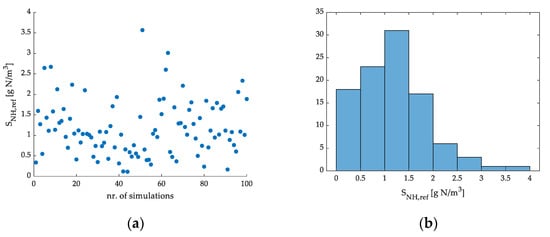
Figure 12.
Scatter plot of the generated and applied SNH,ref data for B1 strategy (a), and a histogram of the data (b).
The obtained data for EFC is presented in Figure 13a,b. By analyzing the data shown in Figure 13a, the lowest and best value for EFC was recorded during simulation nr. 33, representing 0.75, while the worst result was recorded during simulation nr. 51, with a value of 7.17. The histogram presented in Figure 13b contains 14 classes. The category representing the 0.5–1 range includes the most values (55 in total), meaning that the generated values for Qcarb,ref, and SNH,ref managed to maintain the total averaged violation time for all effluent quality parameters under the main reference value of 1 for most of the simulated scenarios.
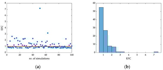
Figure 13.
Scatter plot of the recorded EFC data for the B1 strategy (a), and histogram of the data (b).
The Monte Carlo simulation data analysis, for strategy B1 showed that the lowest obtained value for EFC was 0.75, which was recorded during simulation nr. 34, with the corresponding reference values Qcarb,ref = 2.20 m3/day and SNH,ref = 0.82 g N/m3. The analyzed data show that the environmental impact of the WWTP can be reduced using the optimized version of the B1 strategy (B1,optim1). The data showed that the EFC value for strategy B1,optim1 was better at 4.36% than B1.
In the case of the C1 control strategy, 220 Monte Carlo simulations were performed to identify a better OPC performance regarding the variation of Qcarb,ref, SNH,ref, and TSSref. A higher number of simulations were performed compared to the case of the B1 control strategy, due to the higher importance accorded to the OPC criterion, which summarizes the treatment performance and the cost efficiency of the simulated WWTP.
The generated and applied values of Qcarb,ref are presented in Figure 14a,b. The lowest value generated for Qcarb,ref was 0.0165 m3/day, while the highest was 3.705 m3/day, the average value for the data was 1.263 m3/day, with a corresponding standard deviation of 0.8219 m3/day. The histogram presented in Figure 14b contains 8 classes, where the class regarding the 0.5–1 m3/day range recorded the most generated values (52 values in total); on the other hand, the class of 3.5–5 m3/day range recorded only 2 values.
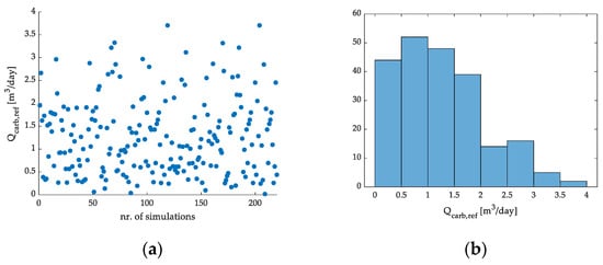
Figure 14.
Scatter plot of the generated and applied Qcarb,ref data for the C1 strategy (a), and histogram of the data (b).
The data regarding the generated and applied values of SNH,ref during the simulations with the C1 control strategy is presented in Figure 15a,b. The data show that the lowest generated value for SNH,ref was 0.1226 g N/m3, and the highest value was 3.734 g N/m3. The average value of the dataset was 1.259 g N/m3, with a standard deviation of 0.7502 g N/m3. The histogram presented in Figure 15b contains eight classes. Most of the generated values fit in the class associated with the 1–1.5 g N/m3 range, including a total of 49 values. The categories with the lowest value counts are the ones representing the 3–3.5 and 3.5–4 g N/m3 range.
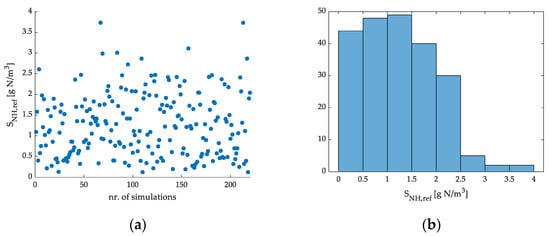
Figure 15.
Scatter plot of the generated and applied SNH,ref data for the C1 strategy (a), and histogram of the data (b).
Figure 16a,b, present the values generated and applied for TSSref during the simulations with strategy C1. The data analysis showed that the lowest value for TSSref was 3998 g SS/m3, and the highest value was 4003 g SS/m3. The identified average value of the data set was 4000 g SS/m3 with a corresponding standard deviation of 0.9767 g SS/m3. Figure 16b shows a histogram with 12 classes. The class representing the 3999.5–4000 g SS/m3 range, includes 47 generated values for TSSref, while categories representing the 4002.5–4003 and 4003–4003.5 g SS/m3 range both include just one value.
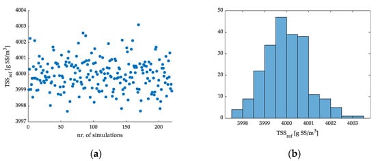
Figure 16.
Scatter plot of the generated and applied TSSref data for the C1 strategy (a), and histogram of the data (b).
The obtained data for OPC are presented in Figure 17a,b. The analysis of the provided data showed that the lowest value for OPC was 0.8062, while the highest value recorded was 1.27. The average value for the data set was below the reference value of 1 (0.9264), with a standard deviation of 0.1093. The histogram presented in Figure 17b contains 10 classes. The data showed that there were 170 out of 220 recorded OPC values that were under the main reference value of 1 (DefCL), this means that the generated values for Qcarb,ref, SNH,ref, and TSSref had a positive impact on the treatment performance and the operational cost of the simulated WWTP.
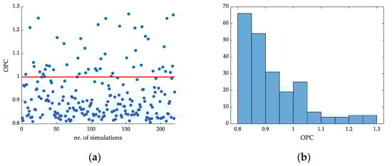
Figure 17.
Scatter plot of the recorded OPC data for the C1 strategy (a), and histogram of the data (b).
The analysis of the database obtained with Monte Carlo simulations for strategy C1 showed that the lowest recorded value for OPC was 0.806, obtained during simulation nr. 185, with the corresponding reference values Qcarb,ref = 3.217 m3/day, SNH,ref = 1.367 g N/m3, and TSSref = 4.0008 g SS/m3. The results obtained with the Monte Carlo simulations indicate that by using the above-provided reference values, a better overall performance of the WWTP can be obtained with the optimized version of the C1 control strategy, hereinafter referred to as C1,optim1, regarding the effluent quality and operational cost. The data analysis showed that the recorded OPC value for the C1,optim1 strategy was 7.27% better than C1.
The required time for running a single BSM2 simulation with the implemented control strategies on the MATLAB-Simulink version R2021 (The MathWorks, Inc., Natick, MA, USA) [35] software platform and on the hardware platform (PC), described in Table 3, was 3 h. For this study, a total of 329 simulations were performed; this means that the total average time required to perform all the simulations was 987 h or 41.125 days.
Table 3.
Specifications of the chosen hardware platform (PC).
A secondary optimization method was applied to fine-tune the results obtained with the Monte Carlo simulations. In this process, all the data obtained during the 220 Monte Carlo simulations with the C1 control strategy were considered.
We wanted to use these parameters in the control of the reactor and as an output parameter, and we considered the OPC computed by Equation (12). Thus, an algorithm was built, as well as an application in MAPLE [36] to obtain the interpolation in the polynomial form that allowed identifying the minimum points of the OPC. A total of 220 simulations were used with the considered parameters, with reference values generated by the Monte Carlo simulations.
The algorithm used in MAPLE was as follows:
Step 1: enter the obtained input data;
Step 2: enter the result data—the values for the OPC;
Step 3: a polynomial interpolation function with mixed terms is considered to eliminate Runge-type oscillations:
Step 4: the quadratic sum of the errors is considered an optimization criterion:
Step 5: choose an order for the polynomial of the variable X = Qcarb,ref—i.e., N1, order for the polynomial of the variable Y = SNH,ref—i.e., N2, order for the polynomial of the variable Z = TSSref—i.e., N3, order for the mixed polynomial in the X and Y variables—i.e., M1, order for the mixed polynomial in the variables Y and Z—i.e., M2, order for the mixed polynomial in the variables Y and Z—i.e., M3f). The expression (9) is constructed, and the unknown parameters are identified , , , , ,
Step 6: the minimum equations for the SS function are obtained through the Lagrange criterion:
Step 7: the system of Equation (17) is obtained
Step 8: solve and obtain the OPC function (15)
Step 9: the global extreme point is obtained using the gradient method:
The best result was obtained for the function with N1 = 3, N2 = 3, N3 = 3, M1 = 3, M2 = 4, M3 = 2 with solutions: A[0]:= 144.6870434; A[1]: = 411.2977385; A[2]: = 74.17256538; A[3]: = 159.0149941; B[1]:= −199.7443299; B[2]: = 190.6667779; B[3]: = −19.05267777; C[1]: = 11.71765377; C[2]: = −8.573052945; C[3]: = 1.681799700; C[4]: = −9.138689286; C[5]: = 6.581981245; C[6]: = −1.273209679; C[7]: = 2.008805234; C[8]: = −1.437730356; C[9]: = 0.2761725198; E[1]: = −0.8144213907 × 10⁻¹; E[2]: = 0.1214935281 × 10⁻⁵; E[3]: = 0.2565978856 × 10⁻⁸; G[1]: = 0.3931651198 × 10⁻¹; G[2]: = −0.1060851966; G[3]: = −0.4503971113 × 10⁻¹; G[4]: = −0.4832290303 × 10⁻⁴; G[5]: = 0.1570879774 × 10⁻⁴; G[6]: = −0.3603226971 × 10⁻⁵; G[7]: = 0.3133588949 × 10⁻⁸; G[8]: = 0.1590685602 × 10⁻⁸; G[9]: = 0.1221893654 × 10⁻⁸; H[1]: = −0.1832604463 × 10⁻¹; H[2]: = −0.4305334064 × 10⁻¹; H[3]: = 0.4581077092 × 10⁻²; H[4]: = 0.1678736180 × 10⁻⁴; H[5]: = −0.9421420125 × 10⁻⁶ (all the other coefficients being null).
The obtained values for the considered parameters show that the minimum point was found at {X = 1.091164454, Y = 1.893995470, Z = 3998.074300}.
For the case of N1 = 4, N2 = 4, and N3 = 3, the solutions are A[0]: = 38.79331422; A[1]:= 54.58356273; A[2]:= −54.89874267; A[3]: = 9.130285634; A[4]: = −0.2418902978 × 10⁻¹; B[1]: = 93.57855588; B[2]:= −8.137547649; B[3]: = 27.74898738; B[4]: = 0.1595063228 × 10⁻¹; C[1]: = 11.66708693; C[2]:= −8.588660175; C[3]: = 1.696953413; C[4]: = −8.898415146; C[5]: = 6.440742530; C[6]: = −1.252483625; C[7]: = 1.915502779; C[8]: = −1.376257336; C[9]: = 0.2653415192; E[1]: = −0.9051494077 × 10⁻²; G[3]: = 0.4950508805 × 10⁻²; G[4]: = −0.9930078603 × 10⁻⁵; G[5]: = 0.5651440646 × 10⁻⁵; G[6]: = −0.1819238506× 10⁻⁵; G[7]: = 0.1569527512 × 10⁻⁸; G[8]: = −0.5129875824× 10⁻⁹; G[9]: = −0.4295523682 × 10⁻¹¹; H[1]: = −0.6654272043 × 10⁻¹; H[2]: = 0.2237734293× 10⁻²; H[3]: = −0.5754304934 × 10⁻²; H[4]: = 0.1195946068 × 10⁻⁴; H[5]: = 0.1399937351 × 10⁻⁵; H[6]: = −0.2369347739 × 10⁻⁵; H[7]: = −0.3651999559 × 10⁻⁹; H[8]: = −0.3075986937 × 10⁻⁹; H[9]: = 0.5058582734 × 10⁻⁹; (all the other coefficients being null.) with abnormal minimum point: X = 2.230214834, Y = 1.749968224, Z = 603.8770144. An implicit plot of this solution is presented in Figure 18.
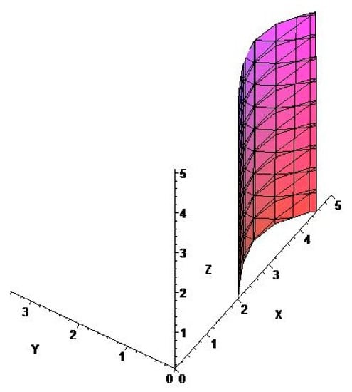
Figure 18.
Implicit plot for the solution (15) in the case of N1 = 4, N2 = 4 and N3 = 3.
For the case of N1 = 5, N2 = 5, and N3 = 5 the solutions for system (9) are A[0]: = −2412.313729; A[1]: = −325.3906894; A[2]: = 545.8958739; A[3]: = −17.27306608; A[4]: = −0.1053491715; C[1]: = 33.25602903; C[2]: = −24.64382008; C[3]: = 4.913422359; C[4]: = −24.45889005; C[5]: = 17.82368140; C[6]: = −3.496600925; C[7]: = 5.135956493; C[8]: = −3.713057323; C[9]: = 0.7211982759; E[1]: = 1.205825370; E[2]: = −0.6723509377 × 10⁻⁴; E[3]: = −0.1717527516 × 10⁻⁷; E[4]: = −0.9038238881 × 10⁻¹²; G[1]: = −0.7120863780 × 10⁻¹; G[2]: = −0.1585462087 × 10⁻¹; G[3]: = 0.1833115999 × 10⁻¹; G[4]: = −0.2219692399× 10⁻⁴; G[5]: = −0.3365876545 × 10⁻⁴; G[6]: = −0.1030361736 × 10⁻⁴; G[7]: = 0.1492116883 × 10⁻⁷; G[8]: = 0.9897112808 × 10⁻⁹; G[9]: = 0.1683003840 × 10⁻⁸; H[1]: = 0.6549770971 × 10⁻¹; H[2]: = 0.2823207027; H[3]: = 0.8535281663 × 10⁻²; H[4]: = −0.1856064094 × 10⁻³; H[5]: = −0.4073615649 × 10⁻⁴; H[6]: = −0.2241036388 × 10⁻⁴; H[7]: = 0.4213196090 × 10⁻⁷; H[8]: = −0.7331183281 × 10⁻⁸; H[9]: = 0.5041925907× 10⁻⁸, with all the other coefficients being null.
The best result obtained for the function with N1 = 3, N2 = 3, N3 = 3, M1 = 3, M2 = 4, and M3 = 2 were put to the test with one simulation where the values for X, Y, and Z, were attributed to the reference values Qcarb,ref, SNH,ref, and TSSref. This configuration of the C1 control strategy was named C1,optim2, for comparison.
The final results regarding the OPC are presented in Figure 19. The analysis of the data shows that C1,optim1 version obtained the best results compared with the unoptimized C1 strategy and with the C1,optim2 version. This indicates that both the applied optimization methods provided an improvement for the C1 strategy, while taking into account the wastewater treatment performance and the cost efficiency of the WWTP.
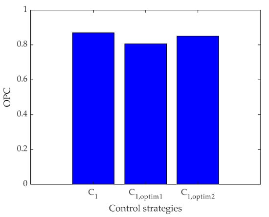
Figure 19.
Final results of OPC for the C1, C1,optim1, and C1,optim2 control strategies.
6. Conclusions
This study proposed evaluating seven control strategies (A1, A2, A3, B1, B2, B3, and C1), which were implemented and tested within the BSM2 framework. The evaluation of these strategies was performed by directly comparing the final results with the results obtained with the DefCL strategy. Thus, both the performance and operating cost, represented by the EQI and OCI, as well as the violation time for specific effluent quality parameters, representing the legal aspect regarding environmental impact, were taken into consideration. Significant importance was given to the influent treatment performance and operating cost, since these indexes are commonly used in the specialized literature.
The implemented control strategies were tested both independently and in combined variants, to identify the strategy that provided the best performance. Strategies A1 and A2 were developed as supporting strategies for DefCL, which remained active during all simulations. Therefore, the BSM2 structure for closed-loop simulations was not excessively affected by the applied strategies. This allowed for a direct comparison with the DefCL strategy, as the strategies could have both a positive and negative impact on EQI and OCI.
The analysis of the results regarding the EFC criterion indicated that the B1 strategy had the lowest negative impact on the environment. However, this does not imply that this strategy was the best in terms of performance and operating cost, as indicated by the OPC criterion, where this strategy ranked in second place.
This paper proposes two new evaluation criteria (EFC and OPC), which proved to be extremely precise and useful when comparing the results of user-made control strategies and the default strategy of BSM2. EFC and OPC were used to simplify and clarify the difference between the reference and the compared results. While OPC was used to summarize the treatment performance and the economic aspect of the simulated WWTP operation, the EFC criteria were used to identify the control strategy that proved to have the smallest negative impact on the environment.
The most important results are indicated by the OPC criterion. Although the EFC criterion suggests that the B1 strategy was the most environmentally friendly, when considering the overall treatment performance and operating costs, this strategy obtained second place. Thus, the strategy with the most significant results was considered to be strategy C1, as indicated by the lowest pollutant loading of the effluent and the lowest operating cost, as confirmed by the values of the additional OPC.
In the attempt to identify the optimal setpoints for the PI controllers, 100 Monte Carlo simulations were performed for strategy B1 and 220 simulations for C1 strategy. The database obtained was analyzed to identify if there were any better results than the one detected during the validation of the best control strategy. The uncertainty analysis of the data obtained with the Monte Carlo simulations indicated that there was a better EFC value recorded for strategy B1 and a better OPC value for strategy C1.
Interestingly, the applied method proved to be useful for identifying the optimal reference values, and this supports the theory that the higher number of Monte Carlo simulations performed, the better the result. Our applied method could also be useful for identifying the main reference values for PI controllers in cases where these values are completely unknown or uncertain.
A secondary optimization method was applied to the Monte Carlo simulation database. The studied system accepts interpolation functions of odd order, an aspect that is relatively easy to understand. This aspect allows the identification of some truthful solutions regarding the optimization of the setpoints of the involved PI controllers.
The obtained results regarding the optimized versions of the B1 and, especially, C1 control strategies proved that these optimization methods could be successfully applied to identify and fine-tune the reference values for PI controllers.
Author Contributions
Conceptualization, B.R. and G.M.; data curation, A.R. and M.A.; formal analysis, G.M.; funding acquisition, M.M.P. and G.M.; investigation, G.D.M. and M.M.P.; methodology, B.R. and G.M.; project administration, B.R.; resources, A.R.; software, B.R. and G.M.; supervision, B.R.; validation, B.R.; visualization, G.D.M. and M.M.P.; writing—original draft, B.R. and A.R.; writing—review and editing, G.M. and M.A. All authors have read and agreed to the published version of the manuscript.
Funding
The work of M.M.P. was supported by the project “PROINVENT”, Contract no. 62487/3 June 2022–POCU/993/6/13–Code 153299, financed by The Human Capital Operational Programme 2014–2020 (POCU), Romania. The work of A.R. and G.M. was supported by the project An Integrated System for the Complex Environmental Research and Monitoring in the Danube River Area, REXDAN, SMIS code 127065, co-financed by the European Regional Development Fund through the Competitiveness Operational Programme 2014–2020, contract no. 309/10 July 2021.
Data Availability Statement
The data are available upon request from the corresponding author.
Acknowledgments
We gratefully acknowledge Ulf Jeppsson from Lund University for generously providing the BSM2 MATLAB/Simulink code.
Conflicts of Interest
The authors declare no conflict of interest.
References
- Lofrano, G.; Brown, J. Wastewater Management through the Ages: A History of Mankind. Sci. Total Environ. 2010, 408, 5254–5264. [Google Scholar] [CrossRef]
- Dorgham, M.M. Effects of Eutrophication. Eutrophication Causes Conseq. Control. 2014, 2, 29–44. [Google Scholar] [CrossRef]
- Kennish, M.J. Nutrient Inputs and Organic Carbon Enrichment: Causes and Consequences of Eutrophication. In Reference Module in Earth Systems and Environmental Sciences; Elsevier: Amsterdam, The Netherlands, 2023. [Google Scholar] [CrossRef]
- Wilkinson, G.M. Eutrophication of Freshwater and Coastal Ecosystems. In Encyclopedia of Sustainable Technologies; Elsevier: Amsterdam, The Netherlands, 2017; pp. 145–152. [Google Scholar] [CrossRef]
- Crini, G.; Lichtfouse, E. Wastewater Treatment: An Overview. In Green Adsorbents for Pollutant Removal; Springer: Cham, Switzerland, 2018; pp. 1–21. [Google Scholar] [CrossRef]
- Calmuc, V.A.; Calmuc, M.; Arseni, M.; Topa, C.M.; Timofti, M.; Burada, A.; Iticescu, C.; Georgescu, L.P. Assessment of Heavy Metal Pollution Levels in Sediments and of Ecological Risk by Quality Indices, Applying a Case Study: The Lower Danube River, Romania. Water 2021, 13, 1801. [Google Scholar] [CrossRef]
- Iticescu, C.; Georgescu, L.P.; Murariu, G.; Circiumaru, A.; Timofti, M. The Characteristics of Sewage Sludge Used on Agricultural Lands. In Recent Advances on Environment, Chemical Engineering and Materials, Proceedings of the AIP Conference Proceedings, Sliema, Malta, 22–24 June 2018; American Institute of Physics: College Park, MD, USA, 2022. [Google Scholar] [CrossRef]
- Calmuc, M.; Calmuc, V.; Arseni, M.; Topa, C.; Timofti, M.; Georgescu, L.P.; Iticescu, C. A Comparative Approach to a Series of Physico-Chemical Quality Indices Used in Assessing Water Quality in the Lower Danube. Water 2020, 12, 3239. [Google Scholar] [CrossRef]
- Alex, J.; Benedetti, L.; Copp, J.; Gernaey, K.V.; Jeppsson, I.; Nopens, I.; Pons, M.N.; Rosen, C.; Steyer, J.P.; Vanrolleghem, P. Benchmark Simulation Model No. 2 (BSM2). Water Sci. Technol. 2018, 2, 1–99. [Google Scholar]
- Santín, I.; Meneses, M.; Pedret, C.; Barbu, M.; Vilanova, R. Nitrous Oxide Reduction in Wastewater Treatment Plants by the Regulation of the Internal Recirculation Flow Rate with a Fuzzy Controller. J. Water Process Eng. 2022, 53, 103802. [Google Scholar] [CrossRef]
- Santín, I.; Vilanova, R.; Pedret, C.; Barbu, M. Global Internal Recirculation Alternative Operation to Reduce Nitrogen and Ammonia Limit Violations and Pumping Energy Costs in Wastewater Treatment Plants. Processes 2020, 8, 1606. [Google Scholar] [CrossRef]
- Luca, L.; Ifrim, G.; Ceanga, E.; Caraman, S.; Barbu, M.; Santin, I.; Vilanova, R. Optimization of the Wastewater Treatment Processes Based on the Relaxation Method. In Proceedings of the 2017 5th International Symposium on Electrical and Electronics Engineering, ISEEE 2017, Galati, Romania, 20–22 October 2017; pp. 1–4. [Google Scholar]
- Tejaswini, E.S.S.; Panjwani, S.; Uday Bhaskar Babu, G.; Seshagiri Rao, A. Model Based Control of a Full-Scale Biological Wastewater Treatment Plant. IFAC-PapersOnLine 2020, 53, 208–213. [Google Scholar] [CrossRef]
- Saagi, R.; Flores-Alsina, X.; Fu, G.; Benedetti, L.; Gernaey, K.V.; Jeppsson, U.; Butler, D. Benchmarking Integrated Control Strategies Using an Extended BSM2 Platform. In Proceedings of the 13th International Conference on Urban Drainage, Sarawak, Malaysia, 7–12 September 2014; pp. 7–12. [Google Scholar]
- Sheik, A.G.; Tejaswini, E.S.S.; Ambati, S.R. Design of Intelligent Control Strategies for Full-Scale Wastewater Treatment Plants with Struvite Unit. J. Water Process. Eng. 2022, 49, 103104. [Google Scholar] [CrossRef]
- Solon, K.; Flores-Alsina, X.; Kazadi Mbamba, C.; Ikumi, D.; Volcke, E.I.P.; Vaneeckhaute, C.; Ekama, G.; Vanrolleghem, P.A.; Batstone, D.J.; Gernaey, K.V.; et al. Plant-Wide Modelling of Phosphorus Transformations in Wastewater Treatment Systems: Impacts of Control and Operational Strategies. Water Res. 2017, 113, 97–110. [Google Scholar] [CrossRef]
- Revollar, S.; Vilanova, R.; Francisco, M.; Vega, P. PI Dissolved Oxygen Control in Wastewater Treatment Plants for Plantwide Nitrogen Removal Efficiency. IFAC-PapersOnLine 2018, 51, 450–455. [Google Scholar] [CrossRef]
- Santín, I.; Pedret, C.; Vilanova, R.; Meneses, M. Advanced Decision Control System for Effluent Violations Removal in Wastewater Treatment Plants. Control Eng. Pract. 2016, 49, 60–75. [Google Scholar] [CrossRef]
- Salles, R.; Mendes, J.; Henggeler Antunes, C.; Moura, P.; Dias, J. Dynamic Setpoint Optimization Using Metaheuristic Algorithms for Wastewater Treatment Plants. In Proceedings of the IECON 2022—48th Annual Conference of the IEEE Industrial Electronics Society, Brussels, Belgium, 17–20 October 2022. [Google Scholar] [CrossRef]
- Santin, I.; Pedret, C.; Meneses, M.; Vilanova, R. Artificial Neural Network for Nitrogen and Ammonia Effluent Limit Violations Risk Detection in Wastewater Treatment Plants. In Proceedings of the 2015 19th International Conference on System Theory, Control and Computing, ICSTCC 2015, Cheile Gradistei, Romania, 14–16 October 2015; pp. 589–594. [Google Scholar] [CrossRef]
- Pisa, I.; Santín, I.; Lopez Vicario, J.; Morell, A.; Vilanova, R. A Recurrent Neural Network for Wastewater Treatment Plant Effluents’ Prediction. In Proceedings of the Actas de las XXXIX Jornadas de Automática, Badajoz, Spain, 5–7 September 2018. [Google Scholar] [CrossRef]
- Benedetti, L.; De Baets, B.; Nopens, I.; Vanrolleghem, P.A. Multi-Criteria Analysis of Wastewater Treatment Plant Design and Control Scenarios under Uncertainty. Environ. Model. Softw. 2010, 25, 616–621. [Google Scholar] [CrossRef]
- Flores-Alsina, X.; Gernaey, K.V.; Jeppsson, U. Global Sensitivity Analysis of the BSM2 Dynamic Influent Disturbance Scenario Generator. Water Sci. Technol. 2012, 65, 1912–1922. [Google Scholar] [CrossRef] [PubMed][Green Version]
- Al, R.; Behera, C.R.; Zubov, A.; Gernaey, K.V.; Sin, G. Meta-Modeling Based Efficient Global Sensitivity Analysis for Wastewater Treatment Plants—An Application to the BSM2 Model. Comput. Chem. Eng. 2019, 127, 233–246. [Google Scholar] [CrossRef]
- Henze, M.; Gujer, W.; Mino, T.; van Loosedrecht, M. Activated Sludge Models ASM1, ASM2, ASM2d and ASM3. Water Intell. Online 2006, 5, 9781780402369. [Google Scholar] [CrossRef]
- Ferrentino, R.; Langone, M.; Fiori, L.; Andreottola, G. Full-Scale Sewage Sludge Reduction Technologies: A Review with a Focus on Energy Consumption. Water 2023, 15, 615. [Google Scholar] [CrossRef]
- IWA Task Group on Mathematical Modelling of Anaerobic Digestion Processes. Anaerobic Digestion Model No. 1. In Scientific and Technical Report No. 13; IWA Publishing: London, UK, 2005; ISBN 9781780403052. [Google Scholar] [CrossRef]
- Batstone, D.J.; Keller, J.; Angelidaki, I.; Kalyuzhnyi, S.V.; Pavlostathis, S.G.; Rozzi, A.; Sanders, W.T.; Siegrist, H.; Vavilin, V.A. The IWA Anaerobic Digestion Model No 1 (ADM1). Water Sci. Technol. 2002, 45, 65–73. [Google Scholar] [CrossRef]
- Farcaş-Flamaropol, D.C.; Surdu, E.; Mare, R. Sludge Dewatering Installations. Hidraulica 2023. Available online: https://hidraulica.fluidas.ro/2023/nr1/68-75.pdf (accessed on 15 June 2023).
- Otterpohl, R.; Raak, M.; Rolfs, T. A Mathematical Model for the Efficiency of the Primary Clarification. In Proceedings of the IAWQ 17th Biennial Int. Conference, Budapest, Hungary, 24–29 July 1994; pp. 205–208. [Google Scholar]
- Otterpohl, R.; Freund, M. Dynamic Models for Clarifiers of Activated Sludge Plants with Dry and Wet Weath-Er Flows. Waf. Sci. Technol. 1992, 26, 1391–1400. [Google Scholar]
- Takács, I.; Patry, G.G.; Nolasco, D. A Dynamic Model of the Clarification-Thickening Process. Water Res. 1991, 25, 1263–1271. [Google Scholar] [CrossRef]
- Jeppsson, U.; Pons, M.N.; Nopens, I.; Alex, J.; Copp, J.B.; Gernaey, K.V.; Rosen, C.; Steyer, J.-P.; Vanrolleghem, P.A. Benchmark Simulation Model No 2: General Protocol and Exploratory Case Studies. Water Sci. Technol. 2007, 56, 67–78. [Google Scholar] [CrossRef] [PubMed]
- Barbu, M.; Santin, I.; Vilanova, R. Applying Control Actions for Water Line and Sludge Line to Increase Wastewater Treatment Plant Performance. Ind. Eng. Chem. Res. 2018, 57, 5630–5638. [Google Scholar] [CrossRef]
- MATLAB Software Version: 9.10.0.1649659 (R2021a) Update 1, Simulink Version 10 March 2021. Available online: https://www.mathworks.com (accessed on 15 June 2023).
- Maplesoft Maple (v. 17)—The Essential Tool for Mathematics. Available online: https://www.maplesoft.com/products/Maple/ (accessed on 28 June 2023).
Disclaimer/Publisher’s Note: The statements, opinions and data contained in all publications are solely those of the individual author(s) and contributor(s) and not of MDPI and/or the editor(s). MDPI and/or the editor(s) disclaim responsibility for any injury to people or property resulting from any ideas, methods, instructions or products referred to in the content. |
© 2023 by the authors. Licensee MDPI, Basel, Switzerland. This article is an open access article distributed under the terms and conditions of the Creative Commons Attribution (CC BY) license (https://creativecommons.org/licenses/by/4.0/).