OPT-RNN-DBSVM: OPTimal Recurrent Neural Network and Density-Based Support Vector Machine

Abstract

When implementing SVMs, two major problems are encountered: (a) the number of local minima of dual-SVM increases exponentially with the number of samples and (b) the computer storage memory required for a regular quadratic programming solver increases exponentially as the problem size expands. The Kernel-Adatron family of algorithms, gaining attention recently, has allowed us to handle very large classification and regression problems. However, these methods treat different types of samples (i.e., noise, border, and core) in the same manner, which makes these algorithms search in unpromising areas and increases the number of iterations as well. This paper introduces a hybrid method to overcome such shortcomings, called the Optimal Recurrent Neural Network and Density-Based Support Vector Machine (Opt-RNN-DBSVM). This method consists of four steps: (a) the characterization of different samples, (b) the elimination of samples with a low probability of being a support vector, (c) the construction of an appropriate recurrent neural network to solve the dual-DBSVM based on an original energy function, and (d) finding the solution to the system of differential equations that govern the dynamics of the RNN, using the Euler–Cauchy method involving an optimal time step. Density-based preprocessing reduces the number of local minima in the dual-SVM. The RNN’s recurring architecture avoids the need to explore recently visited areas. With the optimal time step, the search moves from the current vectors to the best neighboring support vectors. It is demonstrated that RNN-SVM converges to feasible support vectors and Opt-RNN-DBSVM has very low time complexity compared to the RNN-SVM with a constant time step and the Kernel-Adatron algorithm–SVM. Several classification performance measures are used to compare Opt-RNN-DBSVM with different classification methods and the results obtained show the good performance of the proposed method.

1. Introduction

Many classification methods have been proposed in the literature and in a vast array of applications, among them a popular approach called support vector machine based on quadratic programming (QP) [1,2,3]. The difficulty in the implementation of SVMs on massive datasets lies in the fact that the quantity of storage memory required for a regular QP solver increases by an exponential magnitude as the problem size expands.

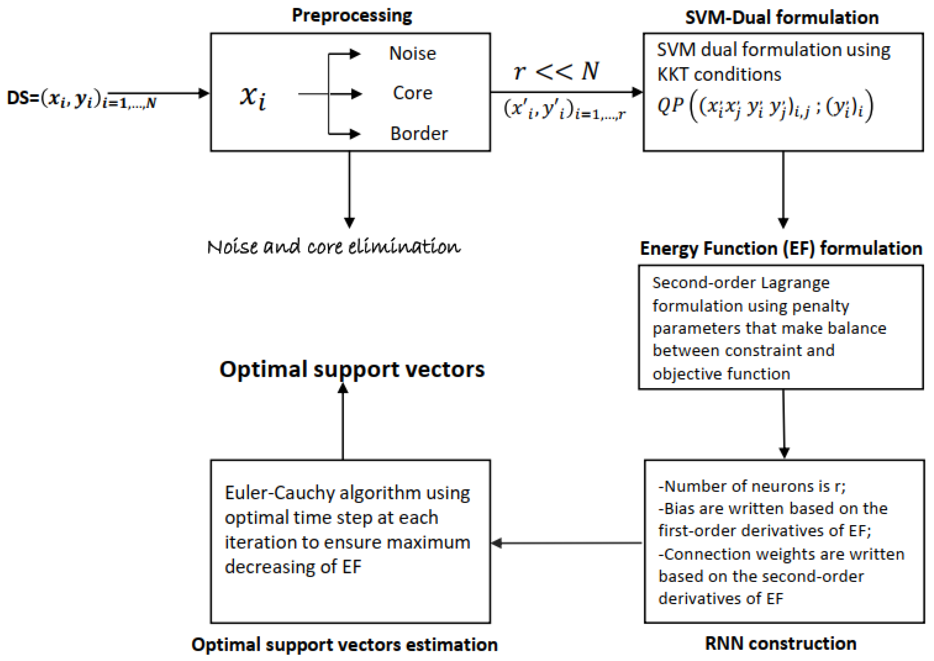
This paper introduces a new type of SVM that implements a preprocessing filter and a recurrent neural network, called the Optimal Recurrent Neural Network and Density-Based Support Vector Machine (Opt-RNN-DBSVM).

SVM approaches are based on the existence of a linear separator, which can be obtained by transforming the data in a higher-dimensional space through appropriate kernel functions. Among all possible hyperplanes, the SVM searches for the one with the most confident separation margin for good generalization. This issue takes the form of a nonlinear constrained optimization problem that is usually handled using optimization methods. Thanks to the Kuhen–Tuker conditions [4], all these methods transform the primal mathematical model into the dual version and use optimization methods to find the support vectors on which the optimal margin is built. Unfortunately, the complexity in time and memory grows exponentially with the size of the datasets; in addition, the number of local minima grows too, which influences the location of the separation margin and the quality of the predictions.

A primary area of research in learning from empirical data through support vector machines (SVMs) and addressing classification and regression issues is the development of incremental learning schemes when the size of the training dataset is massive [5]. Out of many possible candidates, avoiding the usage of regular quadratic programming (QP) solvers, the two learning methods gaining attention recently are iterative single-data algorithms (ISDA) and sequential minimal optimization (SMO) [6,7,8,9]. ISDAs operate from a single sample at hand (pattern-based learning) towards the best fit solution. The Kernel-Adatron (KA) is the primary ISDA for SVMs, using kernel functions to map data to the high-dimensional character space of SVMs [10] and conducting Adatron [11] processing in the character space. Platt’s SMO algorithm is an outlier among the so-called decomposition approaches introduced in [12,13], operating on a two-sample workset of samples at a time. Because the decision for the two-point workset may be determined analytically, the SMO does not require the involvement of standard QP solvers. Due to it being analytically driven, the SMO has been especially popular and is the most commonly utilized, analyzed, and further developed approach. Meanwhile, KA, while yielding somewhat comparable performance (accuracy and computational time) in resolving classification issues, has not gained as much traction. The reason for this is twofold. First, until recently [14], KA appeared to be restricted to classification tasks; second, it lacks the qualities of a robust theoretical framework. KA employs a gradient ascent procedure, and this fact also may have caused some researchers to be suspicious of the challenges posed by gradient ascent techniques in the presence of a perhaps ill-conditioned core array. In [15], lacking bias parameter b, the authors derive and demonstrate the equality of two apparently dissimilar ISDAs, namely a KA approach and an unbiased variant of the SMO training scheme [9], when constructing SVMs possessing positive definite kernels. The equivalence is applicable to both classification and regression tasks and gives additional insights into these apparently dissimilar methods of learning. Despite the richness of the toolbox set up to solve the quadratic programs from SVMs, and with the large amount of data generated by social networks, medical and agricultural fields, etc., the amount of computer memory required for a QP solver from the dual-SVM grows hyper-exponentially, and additional methods implementing different techniques and strategies are more than necessary.

Classical algorithms, namely ISDAs and SMO, do not distinguish between different types of samples (noise, border, and core), which causes searches in unpromising areas. In this work, we introduce a hybrid method to overcome these shortcomings, namely the Optimal Recurrent Neural Network Density-Based Support Vector Machine (Opt-RNN-DBSVM). This method proceeds in four steps: (a) the characterization of different samples based on the density of the datasets (noise, core, and border), (b) the elimination of samples with a low probability of being a support vector, namely core samples that are very far from the borders of different components of different classes, (c) the construction of an appropriate recurrent neural network based on an original energy function, ensuring a balance between the dual-SVM components (constraints and objective function) and ensuring the feasibility of the network equilibrium points [16,17], and (d) the solution of the system of differential equations, managing the dynamics of the RNN, using the Euler–Cauchy method involving an optimal time step. Density-based preprocessing reduces the number of local minima in the dual-SVM. The RNN’s recurrent architecture avoids the need to examine previously visited areas; this behavior is similar to a taboo search, which prohibits certain moves for a few iterations [18]. In addition, the optimal time step of the Euler–Cauchy algorithm speeds up the search for an optimal decision margin. On one hand, two main interesting fundamental results are demonstrated: the convergence of the RNN-SVM to feasible solutions, and the fact that Opt-RNN-DBSVM has very low time complexity compared to Const-RNN-SVM, SMO-SVM, ISDA-SVM, and L1QP-SVM. On the other hand, several experimental studies are conducted based on well-known datasets. Based on several performance measures (accuracy, F1-score, precision, recall), Opt-RNN-DBSVM outperforms recurrent neural network–SVM with a constant time step, the Kernel-Adatron algorithm–SVM family, and well-known non-kernel models. In fact, Opt-RNN-DBSVM improves the accuracy, the F1-score, the precision, and the recall. Moreover, the proposed method requires a very small number of support vectors.

The rest of this paper is organized as follows. Section 2 presents the flowchart of the proposed method. Section 3 gives the outline of our recent SVM version called Density-Based Support Vector Machine. Section 4 presents, in detail, the construction of the recurrent neural network associated with the dual-SVM and the Euler–Cauchy algorithm that implements an optimal time step. Section 5 gives some experimental results. Section 6 presents some conclusions and future extensions of Opt-RNN-DBSVM.

2. The Architecture of the Proposed Method

The Kernel-Adatron (KA) algorithms, namely ISDAs and SMO, treat different types of samples (noise, border, and core) in the same manner (all samples are considered for several iterations and supposed to be a support candidate with uniform probability), which causes searches in unpromising areas and increases the number of iterations. In this work, we introduce an efficient method to overcome these shortcomings, namely Optimal Recurrent Neural Network Density-Based Support Vector Machine (Opt-RNN-DBSVM). This method proceeds in four steps (see Figure 1).

(1)

The characterization of different samples based on the density of the datasets (noise, core, and border); to this end, two parameters are introduced: the size of the neighborhood of the current sample and the threshold that permits such categorization.

(2)

The elimination of samples with a low probability of being a support vector, namely core samples that are very far from the borders of different components of different classes and the noise samples that contain false information about the phenomenon under study. In our previews work [19], we demonstrated that such suppression does not influence the performance of the classifiers.

(3)

The construction of an appropriate recurrent neural network based on an original energy function, allowing a balance between the dual-SVM components (constraints and objective function) and ensuring the feasibility of the network equilibrium points [16,17].

(4)

Solving the system of differential equations, managing the dynamics of the RNN, using the Euler–Cauchy method involving an optimal time step. In this regard, the equation of the future state of each neuron, of the proposed RNN, is introduced into the energy function, which leads to a one-dimension quadratic optimization problem whose solution represents the optimal step of the Euler–Cauchy process that ensures the maximum decrease in the energy function [20]. The components of the produced equilibrium point represent the membership degrees of different samples to the support vector dataset.

Figure 1. Opt_RNN_DBSVM diagram [21,22,23,24].

Figure 1. Opt_RNN_DBSVM diagram [21,22,23,24].

3. Density-Based Support Vector Machine

In the following, let us denote by $BD$ the set of N samples $x_1,\dots ,x_N$ labeled, respectively, by $y_1,\dots ,y_N$, distributed via K class $C_1,\dots ,C_K$. In our case, K=2 and $y_i\in \{-1,+1\}$.

3.1. Classical Support Vector Machine

The hyperplane that the SVM searches must satisfy the equation $w.x_i+b=0$, where w is the weight that defines this SVM separator that satisfies the constraint family given by $\forall i=1,\dots ,N$ $y_i(x_i.w+b)\ge 1$. To ensure the maximum margin, we need to maximize $\frac{2}{\parallel w\parallel }$. As the patterns are not linearly separable, the kernel function K is introduced (which satisfies the Mercer conditions [25]) to transform the data into an appropriate space.

By introducing the Lagrange relaxation and using the Kuhn–Tuker conditions, we obtain a quadratic optimization problem with a single linear constraint that must be solved to determine the support vectors [26].

To address the problem of saturated constraints, some researchers have added the notion of a soft margin [27]. They employ N supplementary slack variables ${\xi }_i\ge 0$ at every constraint $y_i(x_i.w+b)\ge 1$. The sum of the relaxed variables is weighted and included in the cost function:

$$\left\{\begin{array}{c}{\displaystyle Min\frac{1}{2}{\parallel w\parallel }^2+C\sum _{i=1}^N{\xi }_i}\hfill \\ \mathtt{Subject}\mathtt{to}:\hfill \\ y_i(\varphi \left(x_i\right).w+b)\ge 1-{\xi }_i\hfill \\ {\xi }_i\ge 0,\forall i=1,\dots ,N\hfill \end{array}\right.$$

Here, $\varphi$ represents the transformation function derived from the function kernel K. The following dual problem is obtained:

$$\left\{\begin{array}{c}{\displaystyle Max\sum _{i=1}^N{\alpha }_i-\frac{1}{2}\sum _{i=1}^N\sum _{j=1}^N{\alpha }_i{\alpha }_j{y}_i{y}_{j}K(x_i,x_j)}\hfill \\ \mathtt{Subject}\mathtt{to}:\hfill \\ {\displaystyle \sum _{i=1}^N{\alpha }_i{y}_i=0}\hfill \\ 0\le {\alpha }_i\le C,\forall i=1,\dots ,N\hfill \end{array}\right.$$

Several methods can be used to solve this optimization problem: gradient methods, linearization methods, the Frank–Wolf method, the generation column method, the Newton method applied to the Kuhn system, sub-gradient methods, the Dantzig algorithm, the Uzawa algorithm [4], recurrent neural networks [28], hill climbing, simulated annealing, search by calf, A*, genetic algorithms [29], ant colony, and the particle swarm optimization method [30], etc.

Several versions of SVMs are proposed in the literature, e.g., the least squares support vector machine classifiers (LS-SVM) introduced in [21], generalized support vector machine (G-SVM) [22], fuzzy support vector machine [31,32], one-class support vector machine (OC-SVM) [26,33], total support vector machine (T-SVM) [34], weighted support vector machine (W-SVM) [35], granular support vector machine (G-SVM) [36], smooth support vector machine (S-SVM) [37], proximity support vector machine classifiers (P-SVM) [23], multisurface proximal support vector machine classification via generalized eigenvalues (GEP-SVM) [24], and twin support vector machine (T-SVM) [38], etc.

3.2. Density-Based Support Vector Machine (DBSVM)

In this section, a short description of the DBVSM method is given. Let us introduce a real number $r>0$ and the integer $mp>0$, called min-points, and three types of samples are defined: noise points, border points, and interior points (or core points). It is possible to show that the interior points do not change their nature even when they are projected into another space by the kernel functions. Furthermore, such points cannot be selected as support vectors [19].

Definition 1.

Let $S\subseteq {\mathbb{R}}^n$. A point $a\in {\mathbb{R}}^n$ is said to be an interior point (or core point) of S if there exists an $r>0$ such that $B(a,r)\subseteq S$. The set of all interior points of S is denoted by $int\left(S\right)$ or $\stackrel{o}{S}$.

Definition 2.

For a given dataset $BD$, a non-negative real r, and an integer $mp$, there exist three types of samples.

1. 

A sample x is called a $C_i$-noise point $\left(N{P}_i\right)$ if $|C_i\cap B(x,r)|<mp$.

2. 

A sample x is called a $C_i$-core point $\left(C{P}_i\right)$ if $|C_i\cap B(x,r)|\ge mp$ and $x\in \stackrel{o}{\overbrace{envol\left(C_i\right)}}$

3. 

A sample x is called a $C_i$-border point $\left(B{P}_i\right)$ if $|C_i\cap B(x,r)|<mp$ and there exists a $C_i$-core point y such as $x\in B(y,r)$.

Let K be a kernel function allowing us to move from the space ${\mathbb{R}}^n$ to the space ${\mathbb{R}}^N$ using the transformation $\varphi$ (here, $n<N$).

Lemma 1

([19]). If a is a $C_i$-core point for a given ϵ and min-points (mp), then $\varphi \left(a\right)$ is also a $C_i$-core point with an appropriate ${ϵ}^{\prime }$ and the same min-points (mp).

Theorem 1

([19]). A core point is either a noise point or a border point.

Proposition 1

([19]). Let $ϵ>0$ be a real number. The core point set corePoints (minPoints) is a decreasing function for the inclusion operator.

Let $\{{\alpha }_1,\dots ,{\alpha }_n\}$ = $BM\cup CM\cup NM$ be the set of the Lagrange multipliers, where $BM$, $CM$, and $NM$ are the Lagrange multipliers of the border samples, core samples, and noise samples, respectively.

As the elements of $NM$ and $CM$ cannot be selected to be support vectors, the reduced dual problem is given by

$$\left(RD\right)\left\{\begin{array}{c}{\displaystyle Max\sum _{{\alpha }_i\in BM}{\alpha }_i-\frac{1}{2}\sum _{{\alpha }_i\in BM}\sum _{{\alpha }_j\in BM}{\alpha }_i{\alpha }_j{y}_i{y}_{j}K\left(x_i{x}_j\right)}\hfill \\ \mathtt{Subject}\mathtt{to}:\hfill \\ \sum _{{\alpha }_i\in BM}{\alpha }_i{y}_i=0\hfill \\ 0\le {\alpha }_i\le C\forall {\alpha }_i\in BM\forall i=1,\dots ,N\hfill \end{array}\right.$$

In this work, as the RD problem is quadratic with linear constraints, in order to solve this, we use a continuous Hopfield network by proposing an original energy function in the following section [39].

4. Recurrent Neural Network to Find Optimal Support Vectors

The continuous Hopfield network consists of interconnected neurons with a smooth sigmoid activation function (usually a hyperbolic tangent). The differential equation that governs the dynamics of the CHN is

$$\frac{du}{dt}=-\frac{u}{\tau }+W.\alpha +I$$

(1)

where u, $\alpha$, W, and I are, respectively, the vectors of neuron states, the outputs, the weight matrix, and the biases. For a CHN of N neurons, the state $u_i$ and output ${\alpha }_i$ of the neuron i are given by the equation ${\alpha }_i=tanh\left(u_i\right)=f\left(u_i\right)$.

For an initial vector state $u^0\in {\mathbb{R}}^N$, a vector $u^e\in {\mathbb{R}}^N$ is called an equilibrium point of the system 1, if and only if $\exists t^e\in {\mathbb{R}}^{+}$, such as $\forall t\ge t^e$ $u\left(t\right)=u^e$. It should be noted that if the energy function (or Layapunov function) exists, the equilibrium point exists as well. Hopfield proved that the symmetry of the matrix of the weight is a sufficient condition for the existence of the Lyapunov function [40].

4.1. Continuous Hopfield Network Based on Original Energy Function

To solve the obtained dual problem via a recurrent neural network [39,41,42], we propose the following energy function:

$${\displaystyle E({\alpha }_1,\dots ,{\alpha }_N^{\prime })={\beta }_0\sum _{{\alpha }_i\in D}{\alpha }_i-\frac{{\beta }_0}{2}\sum _{{\alpha }_i\in BM}\sum _{{\alpha }_j\in BM}{\alpha }_i{\alpha }_j{y}_i{y}_{j}K\left(x_i{x}_j\right)+{\beta }_1\sum _{{\alpha }_i\in BD}{\alpha }_i{y}_i+\frac{{\beta }_2}{2}{\left(\sum _{{\alpha }_i\in BD}{\alpha }_i{y}_i\right)}^2}$$

To determine the vector of the neurons’ biases, we calculate the partial derivatives of E:

$${\displaystyle \frac{\partial E}{\partial {\alpha }_i}({\alpha }_1,\dots ,{\alpha }_N^{\prime })={\beta }_0-{\beta }_0\sum _{{\alpha }_j\in BM}{\alpha }_j{y}_i{y}_{j}K\left(x_i{x}_j\right)+{\beta }_1{y}_i+{\beta }_2{y}_i\sum _{{\alpha }_j\in BD}{\alpha }_j{y}_j}$$

The components of the bias vector are given by

$$I_i=\frac{\partial E}{\partial {\alpha }_i}\left(0\right)=-{\beta }_0-{\beta }_1{y}_i\forall i=1,\dots N^{\prime }$$

To determine the connection weights W between each neuron pair, the second partial derivative of E is calculated: $\frac{{\partial }^{2}E}{\partial {\alpha }_j\partial {\alpha }_i}({\alpha }_1,\dots ,{\alpha }_{N^{\prime }})=-{\beta }_0{y}_i{y}_{j}K(x_i,x_j)+{\beta }_2{y}_i{y}_j$.

The components of the weight W matrix are given by $W_{i,j}=\frac{{\partial }^{2}E}{\partial {\alpha }_j\partial {\alpha }_i}\left(0\right)={\beta }_0{y}_i{y}_{j}K(x_i,x_j)-{\beta }_2{y}_i{y}_j$.

To calculate the equilibrium point of the proposed recurrent neural network, we use the Euler–Cauchy iterative method:

(1)

Initialization: ${\alpha }_1^0,\dots ,{\alpha }_{N^{\prime }}^0$ and the step ${\rho }^0$ are randomly chosen;

(2)

Given ${\alpha }_1^t,\dots ,{\alpha }_{N^{\prime }}^t$ and the step ${\rho }^t$, the step ${\rho }^{t+1}$ is chosen such that $E^{t+1}$ is the maximum and $u_1,\dots ,u_{N^{\prime }}$ are calculated using $\forall i=1,\dots ,N^{\prime },u_i^{t+1}=u_i^t+{\rho }^{t+1}({\sum }_{j=1,\dots ,N^{\prime }}{W}_{i,j}{\alpha }_j^t+I_i)$

Then, ${\gamma }_1,\dots ,{\gamma }_{N^{\prime }}$ are calculated using the activation function f: ${\gamma }_i=f\left(u_i^{t+1}\right)$.

Then, the ${\alpha }_1^{t+1},\dots ,{\alpha }_{N^{\prime }}^{t+1}$ are given by ${\alpha }^{t+1}=P\left(\gamma \right)$, where P is the projection operator on the set $\{\alpha \in {\mathbb{R}}^{N^{\prime }}/{\sum }_{i=1}^{N^{\prime }}{\alpha }_i{y}_i=0\}$.

(3)

Return to (1) until $\parallel {\alpha }^{t+1}-{\alpha }^t\parallel \le ϵ$, where $0<ϵ$.

Figure 2 shows the connection weights W between each pair of neurons.

Theorem 2.

If $i=j,P_{i,j}=1-\frac{y_i^2}{N^{\prime }}$, else $P_{i,j}=-\frac{y_i{y}_j}{N^{\prime }}$, where ${\displaystyle S=\sum _{i=1,\dots ,N^{\prime }}{y}_i^2}$.

Proof of Theorem 2.

We have $P=I-A^t.{(A.A^t)}^{-1}.A$ and $A=[y_1,\dots ,y_{N^{\prime }}]$.

Then, ${(A.A^t)}^{-1}={([y_1,\dots ,y_{N^{\prime }}].{[y_1,\dots ,y_{N^{\prime }}]}^t)}^{-1}=\frac{1}{N^{\prime }}$ because ${\displaystyle N^{\prime }=\sum _{i=1,\dots ,N^{\prime }}{y}_i^2}$.

Thus $A^t.{(A.A^t)}^{-1}.A=\frac{1}{N^{\prime }}.{[y_1,\dots ,y_{N^{\prime }}]}^t.[y_1,\dots ,y_{N^{\prime }}]$.

Finally, for $i=j$, $P_{i,j}=1-\frac{y_i^2}{N^{\prime }}$, and for $i\ne j,P_{i,j}=-\frac{y_i.y_j}{N^{\prime }}$. □

Concerning the constraint family satisfaction $0\le {\alpha }_i\le C,\forall i=1,\dots ,N$, the activation function is used:

$$f\left(x\right)=C.tanh\left(\frac{x}{\tau }\right)=C.\frac{e^x-e^{-x}}{e^x+e^{-x}},$$

where $\tau$ is supposed to be a very large positive real number, which ensures that $\forall x,-C\le f\left(x\right)\le C$.

Let us consider a kernel function K such that $K(x,x)=C\ne 0$.

Theorem 3.

A continuous Hopfield network has an equilibrium point if $W_{i,i}=0$ and $W_{i,j}=W_{j,i}$.

Theorem 4.

If $C={\displaystyle \frac{{\beta }_2}{{\beta }_0}}$, then CHN-SVM has an equilibrium point.

Proof of Theorem 4.

We have $W_{i,j}=({\beta }_0{K}_{i,j}-{\beta }_2)y_i{y}_j$ and $\forall iandj{W}_{i,j}=W_{j,i}$ because K is symmetric.

On the other hand,

$$W_{i,i}={\beta }_0{y}_{i}K(x_i,x_i)-{\beta }_2{y}_i^2={\beta }_0\times {\displaystyle \frac{{\beta }_2}{{\beta }_0}}-{\beta }_2=0$$

Then, CHN-SVM has an equilibrium point. □

4.2. Continuous Hopfield Network with Optimal Time Step

In this section, we chose, mathematically, the optimal time size in each iteration of the Euler–Cauchy method to solve the dynamical equation of the recurrent neural network proposed in this paper. At the end of the $k^{th}$ iteration, we know ${\alpha }^k$ and let $s_k$ be the next step size, which permits us to calculate ${\alpha }^{k+1}$ using the formula

$${\alpha }^{k+1}={\alpha }^k+s_k\nabla E\left({\alpha }^k\right)$$

and $s_k$ must be chosen such as $E\left({\alpha }^{k+1}\right)\le E\left({\alpha }^k\right)$ at the maximum.

As the activation function of the proposed neural network is the $tanh$, then $\frac{d{\alpha }_i}{dt}=\frac{2}{\tau }{\alpha }_i(1-{\alpha }_i)\nabla E\left(\alpha \right)$.

The matrix form of the energy function is

$$E\left(\alpha \right)={\beta }_0{U}^t\alpha -\frac{{\beta }_0}{2}{\left(\alpha \right)}^{t}T\alpha +{\beta }_1{y}^t\alpha +\frac{{\beta }_2}{2}{\left(y^t\alpha \right)}^2$$

where $U={(1,\dots ,1)}^t\in I{R}^{N^{\prime }}$, $\alpha ={(1,\dots ,1)}^t\in I{R}^{N^{\prime }}$, and $T_{i,j}=y_i{y}_{j}K(x_i,x_j)$ for all i and j.

At the $k^{th}$ iteration, the state ${\alpha }^k$ is known, and ${\alpha }^{k+1}$ is calculated by

$${\alpha }^{k+1}={\alpha }^k+s_k\frac{d{\alpha }^k}{dt}$$

where $s_k$ is the actual time step that must be optimal. To this end, ${\alpha }^{k+1}$ is substituted by ${\alpha }^k+s_k\frac{d{\alpha }^k}{dt}$ in $E\left({\alpha }^{k+1}\right)$:

$$e\left(s_k\right)=E\left({\alpha }^{k+1}\right)=0.5A_k{s}_k^2+B_k{s}_k+C_k$$

where $A_k={\beta }_2{y}^t\frac{d{\alpha }^k}{dt}-{\beta }_0{\left(\frac{d{\alpha }^k}{dt}\right)}^{t}T\frac{d{\alpha }^k}{dt}$,

$B_k={\beta }_0{U}^t\frac{d{\alpha }^k}{dt}-{\beta }_0{\left({\alpha }^k\right)}^{t}T\frac{d{\alpha }^k}{dt}+{\beta }_1{y}^t\frac{d{\alpha }^k}{dt}+{\beta }_2\left(y^t{\alpha }^k\right)\left(y^t\frac{d{\alpha }^k}{dt}\right)$,

$C_k={\beta }_0{U}^t{\alpha }^k-0.5{\beta }_0{\left({\alpha }^k\right)}^{t}T{\alpha }^k+{\beta }_1{y}^t{\alpha }^k+0.5{\beta }_2{\left(y^t{\alpha }^k\right)}^2$.

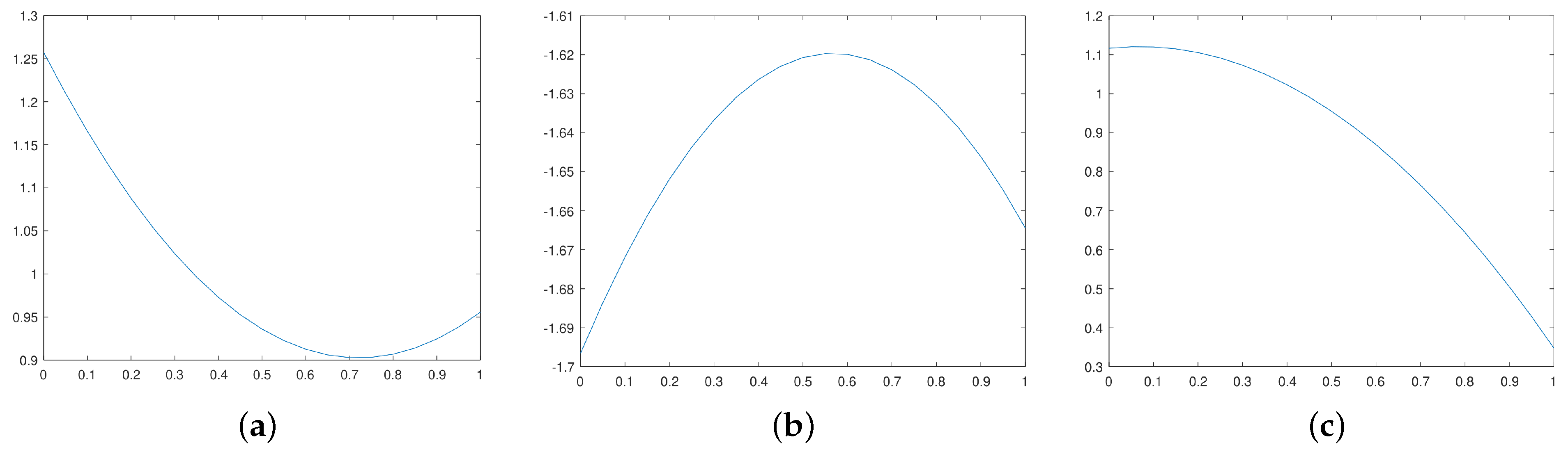
Thus, the best time step is the minimum of $e\left(s_k\right)$. Figure 3a–c gives different cases.

4.3. Opt-RNN-DBSVM Algorithm

In this section, the procedures described in Section 3.2, Section 4.1 and Section 4.2 are summarized into Algorithm 1.

The inputs of Algorithm 1 are the radius r (the size of the neighborhood of the current sample), the minimum of samples $mp$ into $B(Current\_sample,r)$ (which determines the type of this sample), the three Lagrangian parameters ${\beta }_0,{\beta }_1,\mathrm{and}{\beta }_2$ (which allow a compromise between the dual components), the bound C of the SVM [19], and the number of iterations (which represents artificial convergence).

Algorithm 1 processes in three macro-steps: data preprocessing, RNN-SVM construction, and RNN-SVM equilibrium point estimation. The input of the first phase is the initial dataset with labeled samples. Based on r and $mp$, the algorithm determines the types of different samples based on the value of the current sample neighborhood’s discrete size. The output of this phase is a reduced sub-dataset (the initial dataset minus the core samples). The inputs of the second phase are the reduced dataset, the Lagrangian parameters ${\beta }_0$, ${\beta }_1$, ${\beta }_2$, and the SVM bound C. Based on the energy function built in Section 4.1 and on the first and second derivatives, the architecture of CHN-SVM is constructed; the bias and connection weights, which represent the output of this phase, are calculated. These later represent the input of the third phase and the Euler–Cauchy algorithm is used to calculate the degree of membership of different samples in the set of support vectors; to ensure an optimal decrease in the energy function, at each iteration, an optimal step is determined by solving a quadratic one-dimension optimization problem; see Section 4.2. At convergence, the proposed algorithm produces the support vectors based on which Opt-RNN-DBSVM can predict the class of unseen samples.

Algorithm 1 Opt-RNN-DBSVM

Require: $mp,r,{\beta }_0,{\beta }_1,{\beta }_2,C,ITER$ Ensure: $Optimalsupportvectors$  % Density based preprocessing:  $CP\leftarrow ;BP\leftarrow ;NP\leftarrow ;$  for all s in DS do   if $\left|B\right(s,r)\cap DS|>mp$ then    $CP\leftarrow CP\cup \left\{s\right\}$   else if $mp>|B(s,r)\cap DS|>\frac{mp}{2}$ then    $BP\leftarrow BP\cup \left\{s\right\}$   else    $NP\leftarrow NP\cup \left\{s\right\}$   end if  end for  $RDS\leftarrow DS\backslash \{NP\cup CP\}$  % RNN-Building:  $I\leftarrow {\beta }_0+{\beta }_{1}Y$  $W\leftarrow {\beta }_{0}K-{\beta }_2{Y}^{\prime 2}$  % Optimal Euler–Cauchy to RNN stability:  $ste{p}_0=rand(0,1)$  ${\alpha }_0^{\prime }\leftarrow rand(0,1,|RDS\left|\right)$  for k = 1, …, ITER do   $D_k\leftarrow \frac{d{\alpha }^k}{dt}$   $A_k\leftarrow {\beta }_2{y}^t{D}_k-{\beta }_0{\left(D_k\right)}^{t}T{D}_k$   $B_k\leftarrow {\beta }_0{U}^t{D}_k-{\beta }_0{\left({\alpha }^k\right)}^{t}T{D}_k+{\beta }_1{y}^t{D}_k+{\beta }_2\left(y^t{\alpha }^k\right)\left(y^t{D}_k\right)$   $C_k\leftarrow {\beta }_0{U}^t{\alpha }^k-0.5{\beta }_0{\left({\alpha }^k\right)}^{t}T{D}_k+{\beta }_1{y}^t{\alpha }^k+0.5{\beta }_2{\left(y^t{\alpha }^k\right)}^2$   $s_k^{*}\leftarrow argmi{n}_{s\in [0,1]}e\left(s\right)$   ${\alpha }^{k+1}\leftarrow {\alpha }^k+s_k^{*}{D}_k$  end for

Proposition 2.

If N, r, and $ITER$ represent, respectively, the size of a labeled dataset $BD$, the number of remaining samples (output of the preprocessing phase), and the number of iterations, then the complexity of Algorithm 1 is $O(r^2\ast ITER)$.

Proof. 

First, in the preprocessing phase, we calculate, for each sample $(x^i,x^j)$, the distance $d(x^i,x^j)$ and execute N comparisons to determine the type of each sample; thus, the complexity of this phase is $O\left(N^2\right)$.

Second, during $ITER$ iterations, the activation of each neuron is updated using the activation of all the other neurons to solve the reduced dual-SVM; thus, the third phase has complexity of $O(r^2\times ITER)$.

Finally, the complexity of Algorithm 1 is $O\left(N^2\right)+O(r^2\times ITER)$. Let us denote Const-RNN-SVM as the SVM version that implements a recurrent neural network based on a constant time step. Following the same reasoning, the complexity of Const-RNN-SVM is $O(N^2\times ITER)$.

Notes: As the Kernel-Adatron algorithm (KA) is the kernel version of SMO and ISDA, and KA implements two embedded N-loops in each iteration, then the complexity of SMO and ISDA is of [10]. In addition, it is considered that L1QP-SVM implements the numerical linear algebra Gauss–Seidel method [43], which implements two embedded N-loops in each iteration, and thus the complexity of SMO and ISDA is of $O(N^2\times ITER)$. □

For a very large and high-density labeled dataset, we have $r<<N$; thus,

$ITE{R}_{our}<<ITE{R}_{CHN-SVM}$ and $ITE{R}_{our}<<ITE{R}_{L1QP-SVM}$ $ITE{R}_{our}<<ITE{R}_{SMO-SVM}$ and $ITE{R}_{our}<<ITE{R}_{ISDA-SVM}$.

Thus, $complexity\left(our\right)\prec complexity(CHN-SVM)$ and $complexity\left(our\right)\prec complexity(L1QP-SVM)$ $complexity\left(our\right)\prec complexity(SMO-SVM)$, and $complexity\left(our\right)\prec complexity(ISDA-SVM)$.

Firstly, preprocessing the database reduces the number of local minima in the dual-SVM. Secondly, this reduction enables real-time decision making in big data problems. Finally, the optimal time step of the Euler–Cauchy algorithm speeds up the search for an optimal decision margin.

5. Experimentation

In this section, Opt-RNN-DBSVM is compared to several classifiers, Const-RNN-SVM (RNN-SVM using a constant Euler–Cauchy time step), SMO-SVM, ISDA-SVM, L1QP-SVM, and some non-kernel classifiers (Naive Bayes (NB), MLP, KNN, AdaBoostM1 (ABM1), Nearest Center Classifier (NCC), Decision Tree (DT), SGD Classifier (SGDC)). The classifiers were tested on several datasets: IRIS, ABALONE, WINE, ECOLI, BALANCE, LIVER, SPECT, SEED, and PIMA (collected from the University of California at Irvine (UCI) repository [44]). The performance measures used in this study are the accuracy, F1-score, precision, and recall.

5.1. Opt-RNN-DBSVM vs. Const-CHN-SVM

In this subsection, Opt-RNN-DBSVM is compared to Const-RNN-SVM by considering different values of the Euler–Cauchy time step s ∈ {0.1, 0.2, …, 0.9}.

Table 1. Performance Performance of Const-CHN-SVM on different datasets for different values of time step in [0.1, 0.6].

	SVM-CHN $\mathit{s}=0.1$				SVM-CHN $\mathit{s}=0.2$
	Accuracy	F1-Score	Precision	Recall	Accuracy	F1-Score	Precision	Recall
IRIS	95.98	96.66	90.52	92.00	96.66	95.98	91.62	92.00
ABALONE	80.98	40.38	82.00	27.65	80.66	40.38	81.98	27.65
WINE	79.49	78.26	73.52	74.97	79.49	78.26	73.52	74.97
ECOLI	88.05	96.77	97.83	97.33	88.05	97.77	97.83	97.99
BALANCE	79.70	70.7	55.60	62.70	79.70	70.7	55.60	62.70
LIVER	80.40	77.67	77.90	70.08	80.40	77.67	77.90	70.08
SPECT	92.12	90.86	91.33	90.00	97.36	99.60	97.77	1.00
SEED	85.71	83.43	92.70	75.04	85.71	83.43	92.70	75.04
PIMA	79.22	61.90	84.7	49.6	79.22	61.90	83.97	49.6
	SVM-CHN $\mathit{s}=\mathbf{0}.\mathbf{3}$				SVM-CHN $\mathit{s}=\mathbf{0}.\mathbf{4}$
	Accuracy	F1-Score	Precision	Recall	Accuracy	F1-Score	Precision	Recall
IRIS	94.53	95.86	89.66	98.23	95.96	93.88	89.33	95.32
ABALONE	77.99	51.68	83.85	30.88	81.98	41.66	83.56	33.33
WINE	80.23	77.66	74.89	74.97	81.33	77.65	73.11	74.43
ECOLI	88.86	95.65	96.88	97.33	86.77	97.66	97.83	97.95
BALANCE	79.75	70.89	55.96	62.32	79.66	70.45	56.1	66.23
LIVER	80.51	78.33	77.9	70.56	80.40	77.67	77.90	70.08
SPECT	97.63	98.99	97.81	98.56	96.40	98.71	96.83	97.79
SEED	85.71	83.43	92.70	75.88	85.71	83.43	92.70	75.61
PIMA	79.22	61.93	84.82	49.86	79.22	61.90	84.98	49.89
	SVM-CHN $\mathit{s}=\mathbf{0}.\mathbf{5}$				SVM-CHN $\mathit{s}=\mathbf{0}.\mathbf{6}$
	Accuracy	F1-Score	Precision	Recall	Accuracy	F1-Score	Precision	Recall
IRIS	94.53	95.86	89.66	98.23	95.96	93.88	89.33	95.32
ABALONE	78.06	51.83	83.96	40.45	82.1	42.15	83.88	38.26
WINE	80.84	78.26	74.91	75.20	81.39	77.86	73.66	74.47
ECOLI	88.97	95.7	96.91	97.43	86.77	97.66	97.83	97.95
BALANCE	79.89	71.00	56.11	62.72	79.71	70.64	56.33	66.44
LIVER	80.66	78.33	77.9	70.56	80.40	77.67	77.90	70.08
SPECT	91.36	92.60	91.77	84.33	91.36	92.60	91.77	84.33
SEED	84.67	82.96	92.23	74.18	84.11	83.08	92.63	75.48
PIMA	79.12	61.75	84.62	49.86	79.12	61.33	84.68	48.55

and

Table 2. Performance of Const-CHN-SVM on different datasets for different values of time step in [0.7, 0.9].

	SVM-CHN $\mathit{s}=0.7$				SVM-CHN $\mathit{s}=0.8$
	Accuracy	F1-Score	Precision	Recall	Accuracy	F1-Score	Precision	Recall
IRIS	94.53	95.86	89.66	98.23	95.96	93.88	89.33	95.32
ABALONE	77.99	51.68	83.85	30.88	81.98	41.66	83.56	33.33
WINE	80.23	77.66	74.89	74.97	81.33	77.65	73.11	74.43
ECOLI	88.86	95.65	96.88	97.33	86.77	97.66	97.83	97.95
BALANCE	79.75	70.89	55.96	62.32	79.66	70.45	56.1	66.23
LIVER	80.51	78.33	77.9	70.56	80.40	77.67	77.90	70.08
SPECT	94.36	84.60	83.77	85.99	94.36	84.60	83.77	85.99
SEED	85.71	83.43	92.70	75.88	85.71	83.43	92.70	75.61
PIMA	79.22	61.93	84.82	49.86	79.22	61.90	84.98	49.89
	SVM-CHN $\mathit{s}=\mathbf{0}.\mathbf{9}$				CHN-DBSVM Optimal Value of $\mathit{s}$
	Accuracy	F1-Score	Precision	Recall	Accuracy	F1-Score	Precision	Recall
IRIS	95.96	93.88	89.33	95.32	97.96	96.19	95.85	98.5
ABALONE	81.98	41.66	83.56	33.33	98.38	96.07	96.18	93.19
WINE	81.33	77.65	73.11	74.43	96.47	95.96	96.08	96.02
ECOLI	86.77	88.46	90.77	91.19	91.82	97.66	97.83	97.95
BALANCE	79.66	70.45	56.1	66.23	91.31	90.33	89.54	90.89
LIVER	80.40	77.67	77.90	70.08	88.10	85.95	86.00	85.50
SPECT	94.36	84.60	83.77	85.99	95.55	86.20	85.28	86.31
SEED	85.71	83.43	86.18	75.61	88.90	84.31	92.70	84.40
PIMA	79.22	61.90	75.90	49.89	79.87	68.04	84.98	62.05

show the different values of accuracy, F1-score, precision, and recall on the considered datasets. These results show the superiority of Opt-RNN-DBSVM over Const-CHN-SVM (step∈ STEP = {0.1, 0.2, …, 0.9}). In fact, this superiority is quantified as follows:

$$3.43\%=\underset{(s,d)\in STEP\times DATA}{max}(accuracy(Opt-RNN-DBSVM\left(s\right))-accuracy(const-RNN-SVM))$$

$$2.31\%=\underset{(s,d)\in STEP\times DATA}{max}(F1Score(Opt-RNN-DBSVM\left(s\right))-F1Score(const-RNN-SVM))$$

$$7.52\%=\underset{(s,d)\in STEP\times DATA}{max}(precision(Opt-RNN-DBSVM\left(s\right))-precision(const-RNN-SVM))$$

$$6.5\%=\underset{(s,d)\in STEP\times DATA}{max}(recall(Opt-RNN-DBSVM\left(s\right))-recall(const-RNN-SVM))$$

where $DATA$ is the set of different considered data. These results are not unexpected, because Opt-RNN-SVM ensures an optimal decrease in the CHN energy function at each step. This superiority is normal, since a single time step of the Euler–Cauchy algorithm does not explore all the regions of the solution space of the dual problem associated with the SVM, and it also causes premature convergence to a poor local solution. On the other hand, the variable optimal time step of this algorithm allowed a higher-order decay in the energy function of the RNN associated with the dual-SVM.

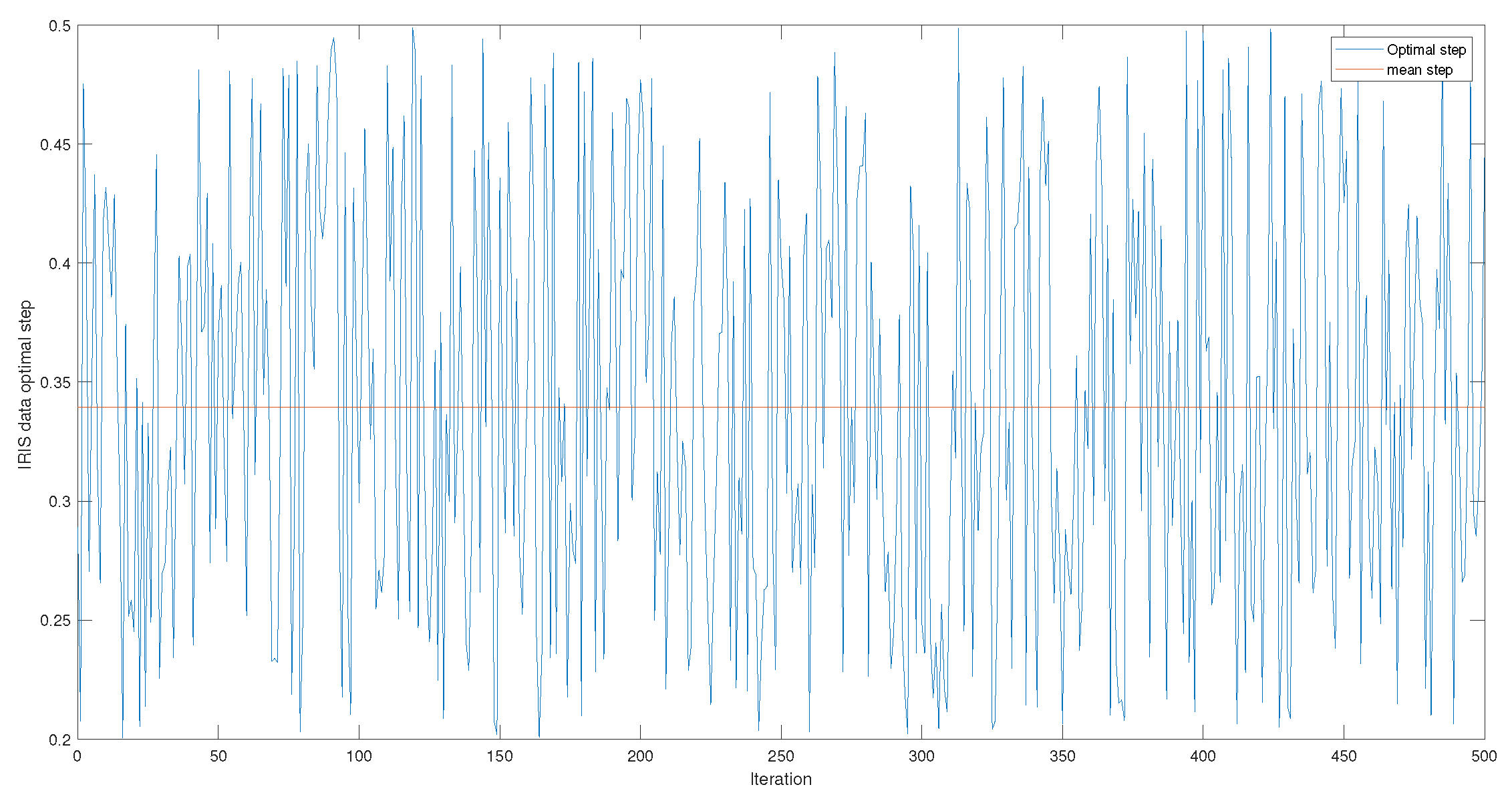
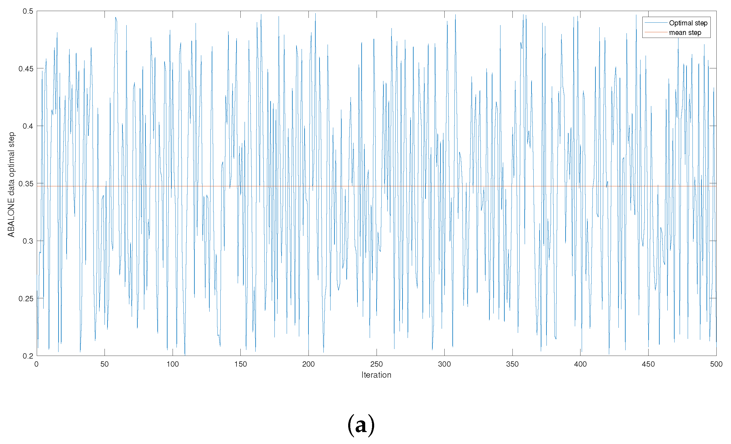
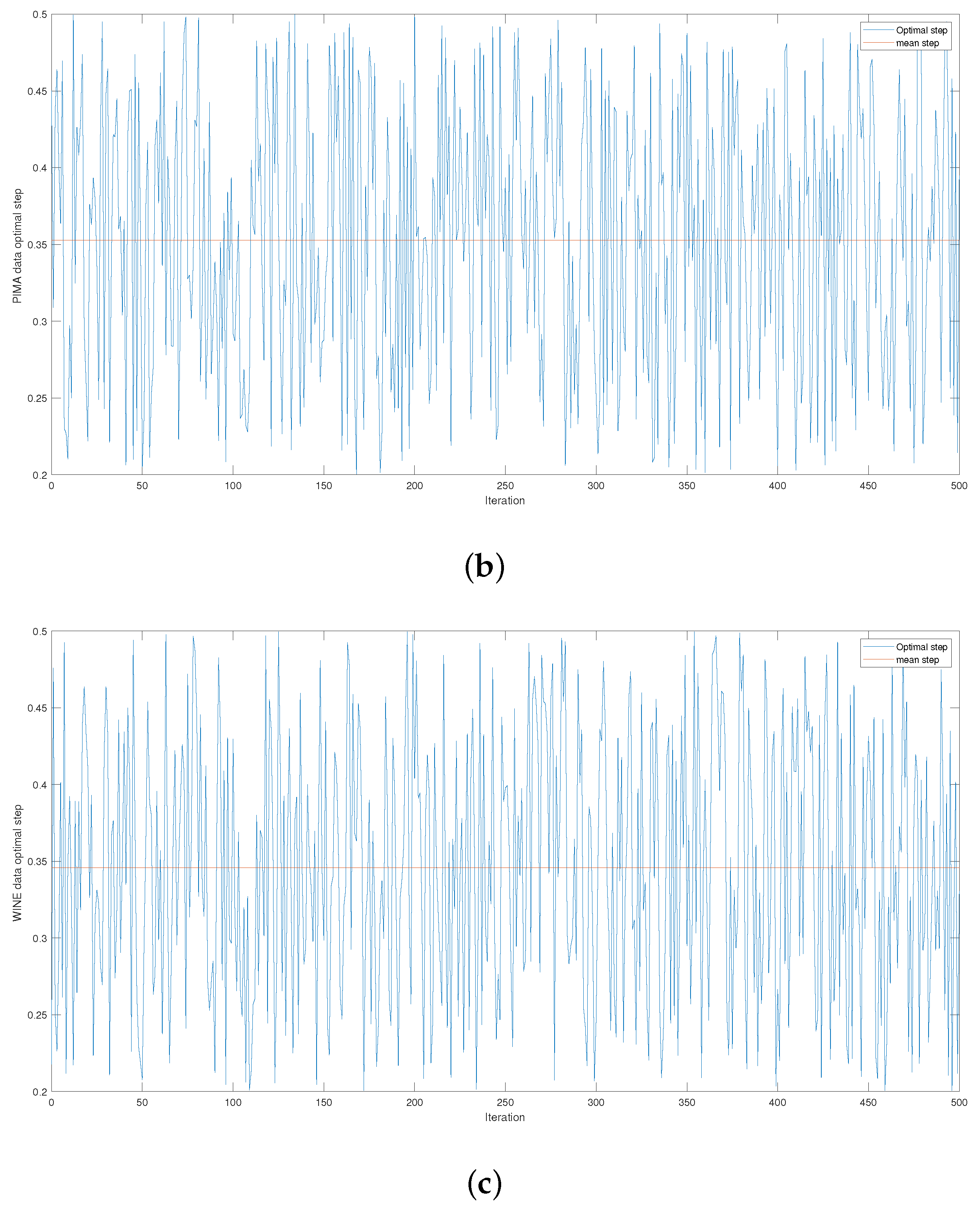
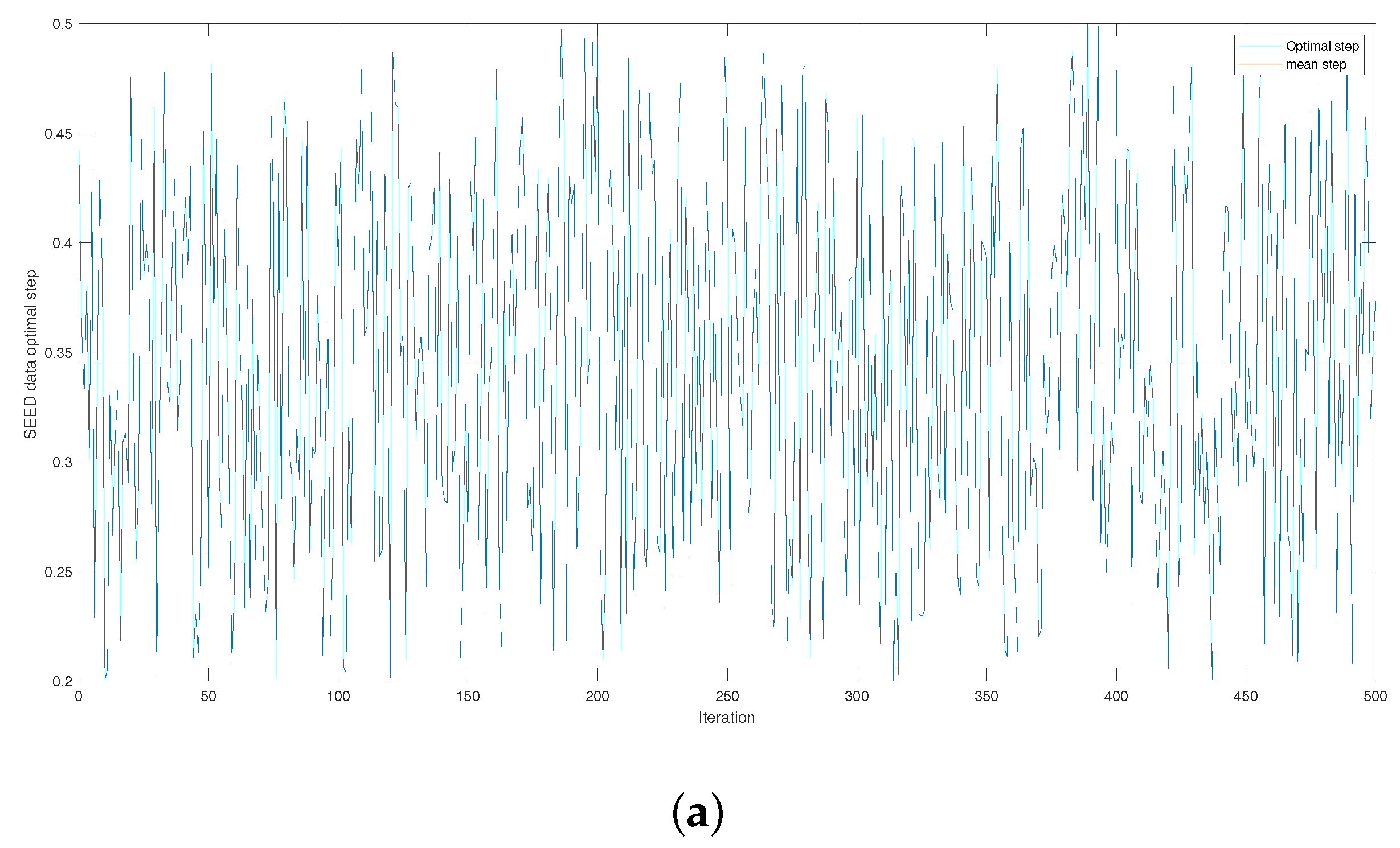
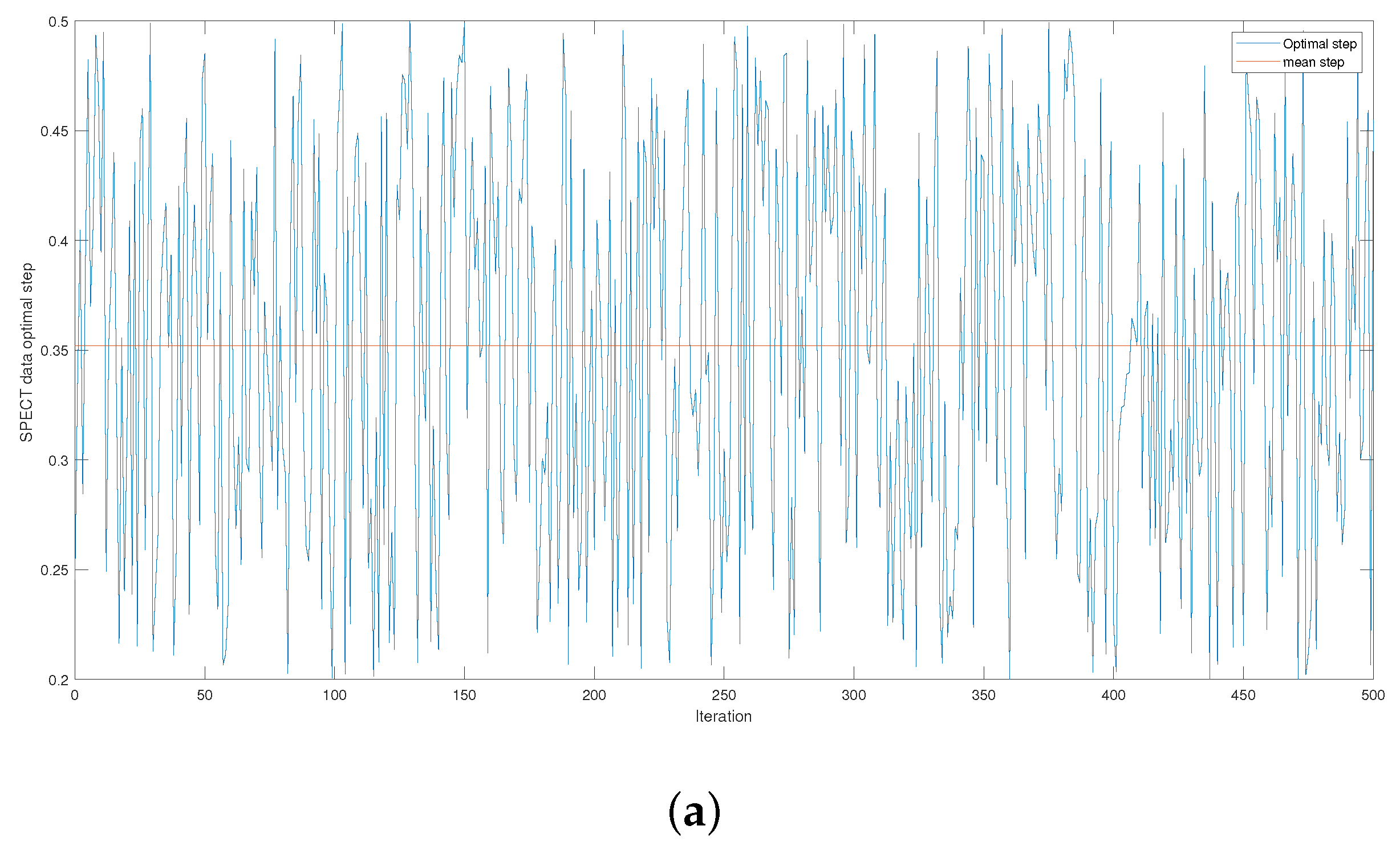
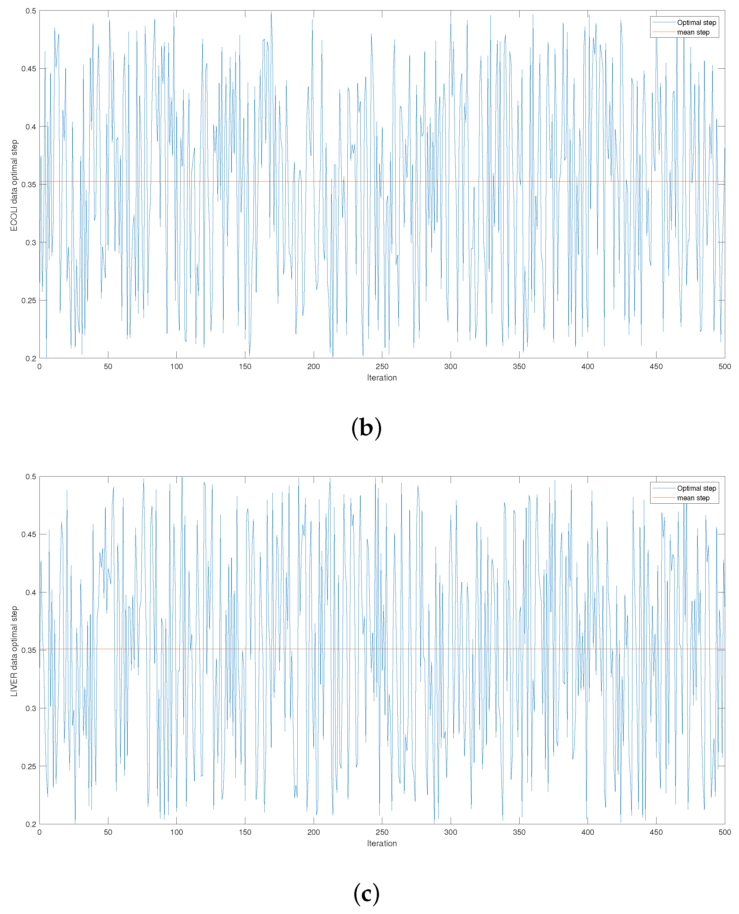
Figure 4 and Figure A1, Figure A2 and Figure A3 give the series of optimal steps generated by Opt-RNN-DBSVM during iterations for different datasets. It is noted that all the optimal steps are taken from the interval $[0.3;0.4]$, which explains why a single constant time step of the Euler–Cauchy algorithm can never produce satisfactory support vectors compared to Opt-RNN-DBSVM. However, this simulation provides an optimal domain for those using a CHN based on a constant time step instead of taking a random time step from $[0;1]$.

5.2. Opt-RNN-DBSVM vs. Classical Optimizer–SVM

In this section, we give the performance of different Classical Optimizer–SVM models (L1QP-SVM, ISDA-SVM, and SMO-SVM) applied to several datasets and compare the number of support vectors obtained by the different Classical Optimizer–SVM models and Opt-RNN-SVM.

Table 3. Performance of Classical Optimizer–SVM on different datasets.

	L1QP-SVM				ISDA-SVM
	Accuracy	F1-Score	Precision	Recall	Accuracy	F1-Score	Precision	Recall
IRIS	71.59	62.02	70.80	55.17	82.00	83.64	76.67	92.00
ABALONE	74.15	70.80	71.48	59.30	83.70	68.22	70.00	80.66
WINE	72.90	65.79	75.53	60.11	66.08	65.80	66.00	70.02
ECOLI	66.15	55.89	61.33	41.30	51.60	48.30	33.33	51.39
BALANCE	65.20	53.01	60.51	41.22	50.44	58.36	68.32	60.20
LIVER	64.66	52.06	60.77	40.44	50.00	48.00	62.31	51.22
SPECT	70.66	62.02	67.48	50.11	77.60	71.20	75.33	70.11
SEED	70.51	58.98	67.30	45.30	80.66	81.25	79.80	79.30
PIMA	65.18	53.23	60.88	39.48	49.32	44.33	48.90	50.27
	SMO-SVM				CHN-DBSVM Optimal Value of $\mathit{s}$
	Accuracy	F1-Score	Precision	Recall	Accuracy	F1-Score	Precision	Recall
IRIS	71.59	62.02	70.80	55.17	97.96	96.19	95.85	98.5
ABALONE	74.15	70.80	71.48	59.30	98.38	96.07	96.18	93.19
WINE	72.90	65.79	75.53	60.11	96.47	95.96	96.08	96.02
ECOLI	66.15	55.89	61.33	41.30	91.82	88.46	90.77	91.19
BALANCE	65.20	53.01	60.51	41.22	91.31	90.33	89.54	90.89
LIVER	64.66	52.06	60.77	40.44	88.10	85.95	86.00	85.50
SPECT	70.66	62.02	67.48	50.11	95.55	86.20	85.28	86.31
SEED	70.51	58.98	67.30	45.30	88.90	84.31	86.18	84.40
PIMA	65.18	53.23	60.88	39.48	79.87	68.04	75.90	62.05

gives the values of accuracy, F1-score, precision, and recall for Classical Optimizer–SVM on different datasets. The results show the superiority of Opt-RNN-DBSVM. Indeed, when considering each of the performance measures, the proposed method achieves remarkable improvements of 30% for accuracy and F1-score, 50% for precision, and 40% for recall.

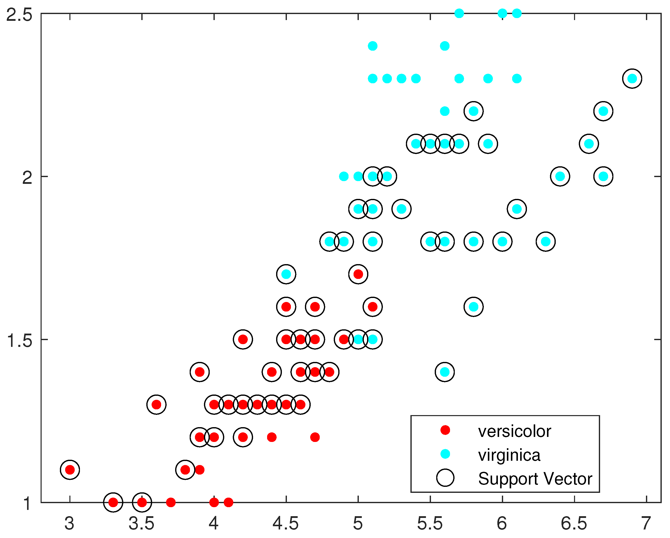
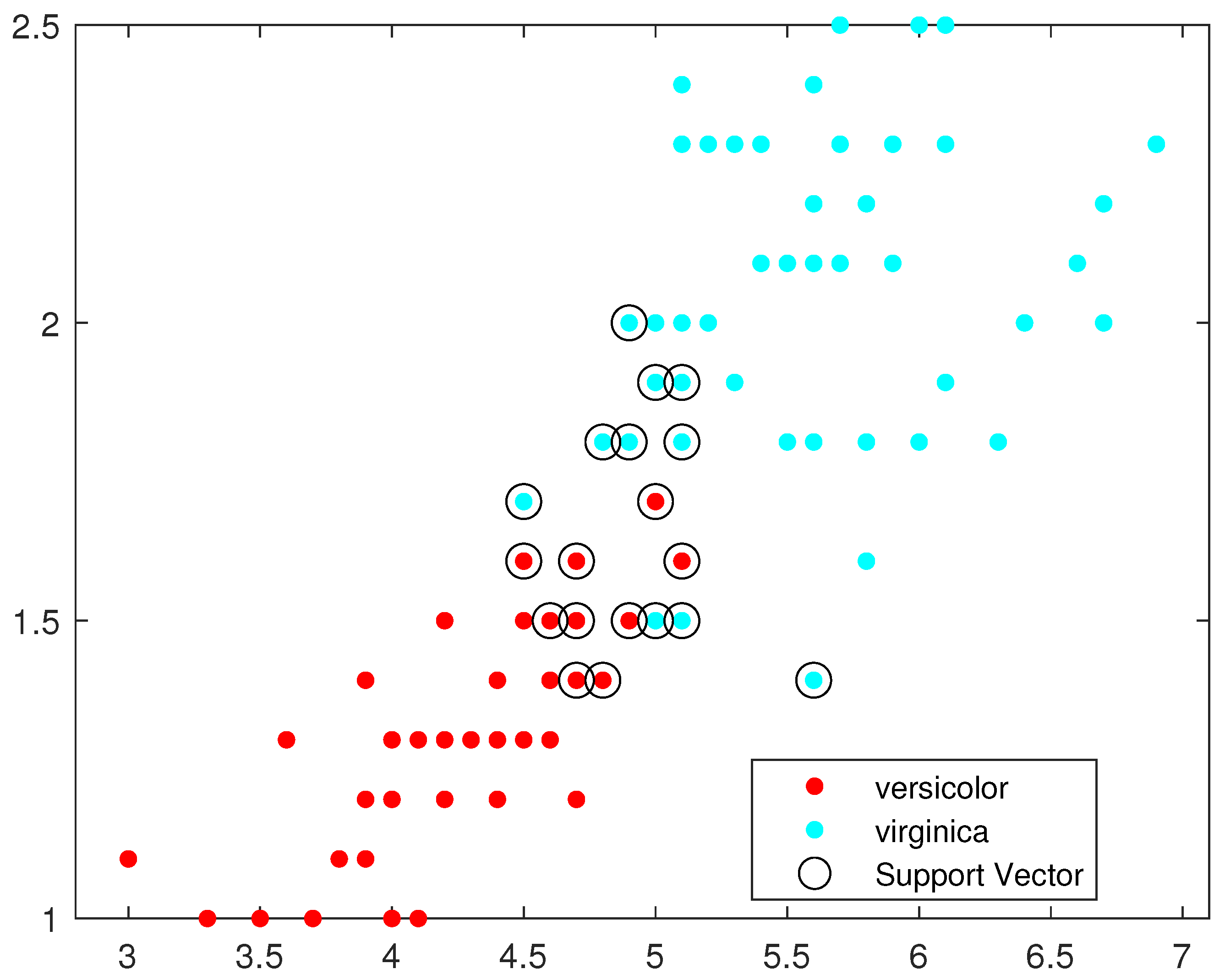
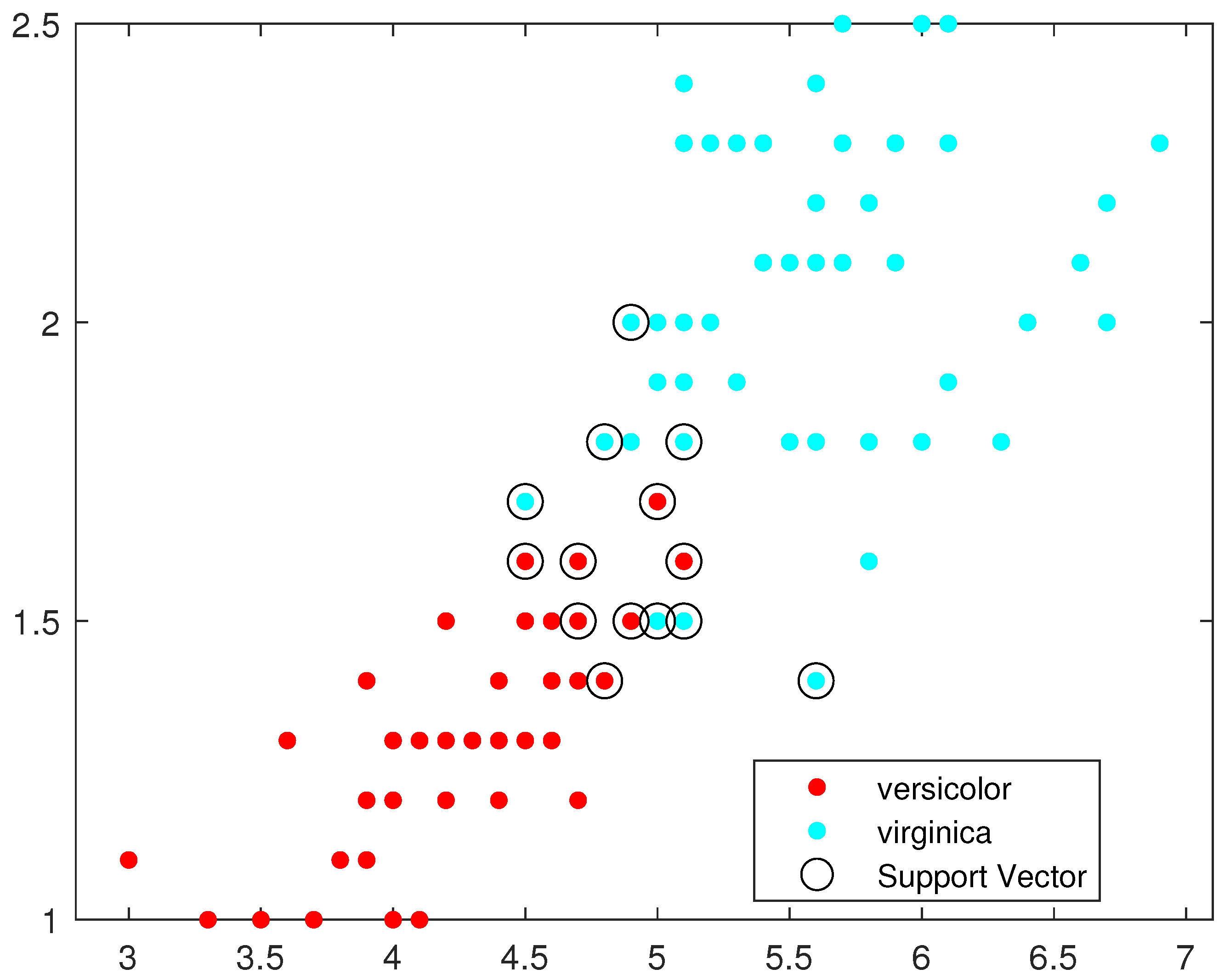
Figure 5, Figure 6, Figure 7 and Figure 8 illustrate, respectively, the support vectors obtained using L1QP-SVM, L1QP-SVM, SMO-SVM, and Opt-RNN-SVM applied to the IRIS data. We note that (a) ISDA considers more than $96\%$ as support vectors, which is an exaggeration; (b) L1QP and SMO use a reasonable number of samples as support vectors, but most of them are duplicated; and (c) thanks to the preprocessing, Opt-RNN can reduce the number of support vectors by more than $32\%$, compared to SMO and L1QP, which allows it to overcome the over-learning phenomenon encountered with SMO and L1QP. In this sense, this reasonable number of support vectors used by Opt-RNN-DBSVM will speed up the online predictions of systems that implement these support vectors, especially with regard to to sentiment analysis, which manipulates very long texts.

To analyze these results further and to evaluate the performance of multiple kernel classifiers, regardless of the data type, we perform the Friedman test to verify the statistical significance of the proposed method compared to other methods with respect to the derived mean rankings [11]. The null hypothesis is given by $H_0^{ker}$, i.e., “The kernel classifiers Opt-RNN-DB, SMO, ISDA, and L1QP perform similarly in mean rankings without a significant difference”. The considered degree of freedom of the Friedman test is 3 (number of kernel classifiers −1). The significance level is 0.05 and the considered confidence interval is 95%. Three performance measures are considered (accuracy, F1-score, precision).

Considering the accuracy measure, the average rank of the four kernel methods is given in brackets: Opt-RNN-DB(4), SMO(2.06), and L1QP(2.06), and ISDA(1.89). Opt-RNN-DB has the highest ranking, followed by SMO and L1QP. Considering the F1-score, the average rank of the four kernel methods is given in brackets: Opt-RNN-DB(4), ISDA(2.11), SMO(1.94), and L1QP(1.94). Opt-RNN-DB has the highest ranking, followed by ISDA. Considering the precision measure, the average rank of the four kernel methods is given in brackets: Opt-RNN-DB(4), ISDA(2.11), SMO(1.94), and L1QP(1.94). Opt-RNN-DB has the highest ranking, followed by ISDA.

Table 4. Results of Friedman test on the kernel SVM classifiers.

Opt-RNN-DB vs.	p-Value (Accuracy)	p-Value (F1-Score)	p-Value (Precision)
SOM	0.008	0.004	0.004
L1QP	0.008	0.004	0.004
ISDA	0.003	0.011	0.011

gives the results of the Friedman test on the kernel SVM classifiers (SOM, L1QP, ISDA) considering different performance measures. The null hypothesis $H_0^{ker}$ is rejected for all these kernel classifiers at a significance level of $\alpha$ = 0.05, indicating that the proposed hybrid classifier outperforms all other kernel classifiers. In this regard, the performance of ISDA-SVM is the closest to that of the Opt-RNN-DBSVM classifier.

5.3. Opt-RNN-DBSVM vs. Non-Kernel Classifiers

In this section, we compare Opt-RNN-DBSVM to several non-kernel classifiers, namely Naive Bayes [45], MLP [46], KNN [47], AdaBoostM1 [48], Decision Tree [49], SGD Classifier [50], Nearest Centroid Classifier [50], and Classical SVM [51].

Table A1. Comparison between Opt-RNN-DBSVM and different classification methods on the IRIS and ABALONE datasets.

IRIS
Method	Accuracy	F1-Score	Precision	Recall
Naive Bayes	90.00	87.99	77.66	1.00
MLP	26.66	0.00	0.00	0.00
KNN	96.66	95.98	91.62	1.00
AdaBoostM1	86.66	83.66	71.77	1.00
Decision Tree	69.25	76.12	70.01	69.55
SGD Classifier	76.66	46.80	1.00	30.10
Random Forest Classifier	90.00	87.99	77.66	1.00
Nearest Centroid Classifier	96.66	95.98	91.62	1.00
Classical SVM	96.66	95.98	91.62	1.00
Opt-RNN-DBSVM	97.96	92.19	95.85	96.05
ABALONE
Method	Accuracy	F1-Score	Precision	Recall
Naive Bayes	68.89	51.19	41.37	67.33
MLP	62.91	47.63	36.32	47.63
KNN	81.93	53.74	70.23	43.02
AdaBoostM1	82.29	55.99	70.56	55.06
Decision Tree	76.79	51.33	52.06	49.63
SGD Classifier	80.86	64.74	58.08	70.57
Nearest Centroid Classifier	76.07	64.79	62.60	61.15
Random Forest Classifier	82.28	57.56	71.11	48.34
Classical SVM	80.98	40.38	82.00	27.65
Opt-RNN-DBSVM	98.38	96.07	96.18	93.19

,

Table A2. Comparison between Opt-RNN-DBSVM and different classification methods on the WINE and ECOLI datasets.

WINE
Method	Accuracy	F1-Score	Precision	Recall
Naive Bayes	78.48	75.96	74.17	74.89
MLP	67.73	72.67	51.52	43.64
KNN	81.84	79.85	78.35	79.00
AdaBoostM1	88.20	70.60	81.64	76.21
Decision Tree	83.02	81.42	79.36	80.22
SGD Classifier	68.40	83.95	52.28	44.81
Nearest Centroid Classifier	73.44	70.75	72.33	71.23
Classical SVM	79.49	78.26	73.52	74.97
Opt-RNN-DBSVM	96.47	95.96	96.08	96.02
ECOLI
Method	Accuracy	F1-Score	Precision	Recall
Naive Bayes	82.08	97.11	1.00	95.66
MLP	55.22	71.45	55.00	1.00
KNN	89.55	99.87	1.00	97.02
AdaBoostM1	70.14	87.21	77.73	1.00
Decision Tree	70.14	83.71	82.03	84.19
SGD Classifier	86.56	96.33	1.00	92.01
Random Forest Classifier	85.07	96.11	97.00	95.66
Nearest Centroid Classifier	82.08	97.28	1.00	95.39
Classical SVM	88.05	97.77	97.83	97.99
Opt-RNN-DBSVM	91.82	88.46	90.77	91.19

,

Table A3. Comparison between Opt-RNN-DBSVM and different classification methods on the BALANCE and LIVER datasets.

BALANCE
Method	Accuracy	F1-Score	Precision	Recall
Naive Bayes	79.3	67.2	62.50	69.40
MLP	76.6	61.10	57.40	68.30
KNN	80.90	68.40	64.50	66.60
AdaBoostM1	81.10	69.20	70.60	66.50
Decision Tree	79.90	64.80	72.80	68.70
SGD Classifier	69.03	65.62	66.15	65.83
Nearest Centroid Classifier	66.54	65	66.66	64.89
Classical SVM	79.70	70.7	55.60	62.70
Opt-RNN-DBSVM	91.31	90.33	89.54	90.89
LIVER
Method	Accuracy	F1-Score	Precision	Recall
Naive Bayes	71.66	71.90	71.45	70.80
MLP	61.50	63.15	72.70	68.88
KNN	50.50	71.20	69.81	53.90
AdaBoostM1	88.50	89.37	89.99	79.39
Decision Tree	39.26	45.39	48.38	48.76
SGD Classifier	49.80	60.00	49.49	50.22
Nearest Centroid Classifier	66.50	63.30	60.20	61.87
Classical SVM	80.40	77.67	77.90	70.08
Opt-RNN-DBSVM	88.10	85.95	86.00	85.50

,

Table A4. Comparison between Opt-RNN-DBSVM and different classification methods on the SPECT and SEED datasets.

SPECT
Method	Accuracy	F1-Score	Precision	Recall
Naive Bayes	63.15	77.40	96.33	65.94
MLP	97.36	99.60	97.77	1.00
KNN	92.10	96.80	97.80	95.90
AdaBoostM1	94.73	97.99	97.55	97.50
Decision Tree	86.84	93.89	97.55	89.48
SGD Classifier	97.36	99.60	97.77	1.00
Random Forest Classifier	97.36	99.60	97.77	1.00
Nearest Centroid Classifier	57.89	72.20	1.00	72.28
Classical SVM	97.36	99.60	97.77	1.00
Opt-RNN-DBSVM	97.36	99.60	97.77	1.00
SEED
Method	Accuracy	F1-Score	Precision	Recall
Naive Bayes	85.71	79.76	92.55	69.20
MLP	30.95	0.00	0.00	0.00
KNN	85.71	79.24	73.39	85.40
AdaBoostM1	95.23	93.40	87.44	1.00
Decision Tree	92.85	90.88	1.00	81.00
Random Forest Classifier	92.85	90.88	1.00	81.00
SGD Classifier	85.71	86.76	79.55	94.20
Nearest Centroid Classifier	85.71	79.28	92.70	75.77
Classical SVM	85.71	83.43	92.70	75.04
Opt-RNN-DBSVM	96.88	97.09	96.76	1.00

,

Table A5. Comparison between Opt-RNN-DBSVM and different classification methods on the PIMA and Germany Diabetes datasets.

PIMA
Method	Accuracy	F1-Score	Precision	Recall
Naive Bayes	79.3	70.40	74.2	66.50
MLP	66.23	13.33	57.1	8.40
KNN	74.90	66.60	68.4	64.50
AdaBoostM1	72.72	60.37	60.8	60.80
Decision Tree	70.77	52.63	60.2	47.60
SGD Classifier	37.66	52.47	36.98	1.00
Nearest Centroid Classifier	63.63	48.14	47.01	49.55
Classical SVM	79.22	61.90	84.7	49.6
Opt-RNN-DBSVM	79.87	68.04	75.90	62.05
Germany Diabetes Dataset
Method	Accuracy	F1-Score	Precision	Recall
Naive Bayes	81.66	87.19	79.37	77.33
MLP	63.28	54.24	50.39	56.40
KNN	68.08	67.88	76.30	66.00
AdaBoostM1	91.95	90.66	92.56	90.06
Decision Tree	55.66	53.74	59.93	50.02
SGD Classifier	79.96	79.74	70.08	78.57
Nearest Centroid Classifier	86.71	82.63	89.32	85.63
Classical SVM	78.5	59.81	74.10	50.99
Opt-RNN-DBSVM	99.5	99.7	1.00	98.00

give the values of the measures accuracy, F1-score, precision, and recall for the considered datasets. Considering each of these performance measures, Opt-RNN-DBSVM permits remarkable improvements and clearly outperforms the other methods. The large number of classifiers and datasets makes it difficult to demonstrate this superiority without employing statistical methods.

To analyze these results further and to evaluate the performance of non-kernel classifiers (Naive Bayes (NB), MLP, KNN, AdaBoostM1 (ABM1), Nearest Centroid Classifier (NCC), Decision Tree (DT), SGD Classifier (SGDC)) compared to Opt-RNN DBSVM, regardless of the data type, we perform the Friedman test to verify the statistical significance of the proposed method compared to other methods with respect to the derived mean rankings. Three performance measures are considered (accuracy, F1-score, precision).

The null hypothesis is given by $H_0^{nker}$, i.e., “The classifiers NB, MLP, KNN, ABM1, NCC, DT, SGDC, Opt-RNN-DBSVM perform similarly in mean rankings without a significant difference”.

The considered degree of freedom of the Friedman test is 7 (number of non-kernel classifiers −1). The significance level is 0.05 and the considered confidence interval is 95%.

Considering the accuracy measure, the average rank of the four kernel methods is given in brackets: Opt-RNN-DBSVM(7.80), ABM1(5.2), KNN(5.2), NB(4.4), NCC(3.95), SGDC(3.55), DT(3.5), and MLP(2.4). Opt-RNN-DB has the highest ranking, followed by ABM1(5.2) and KNN(5.2). Considering the F1-score, the average rank of the four kernel methods is given in brackets: Opt-RNN-DBSVM(7.1), ABM1(5.2), KNN(5.05), NB(4.8), SGDC(4.6), NCC(4.05), DT(3.1), and MLP(2.1). Opt-RNN-DB has the highest ranking, followed by ABM1 and KNN. Considering the precision measure, the average rank of the four kernel methods is given in brackets: Opt-RNN-DBSVM(7.1), NCC(5.3), ABM1(5.15), KNN(4.9), NB(4.25), SGDC(3.95), DT(3.25), and MLP(2.1). Opt-RNN-DB has the highest ranking, followed by NCC and ABM1.

Table 5. Results of Friedman test on non-kernel classifiers.

Opt-RNN-DB vs.	p-Value (Accuracy)	p-Value (F1-Score)	p-Value (Precision)
Naive Bayes	0.054	0.022	0.026
MLP	0.00	0.00	0.00
KNN	0.018	0.061	0.045
AdaBoostM1	0.018	0.083	0.075
Nearest Centroid Classifier	0.012	0.15	0.1
Decision Tree	0.002	0.007	0.012
SGD Classifier	0.003	0.022	0.004

gives the results of the Friedman test on the non-kernel classifiers (NB, MLP, KNN, ABM1, NCC, DT, and SGDC) considering three performance measures (accuracy, F1-score, and precision). The null hypothesis $H_0^{nker}$ is rejected for all these classifiers at a significance level of $\alpha$ = 0.05, indicating that the proposed hybrid classifier outperforms all other non-kernel classifiers. In this regard, the performance of ABM1 is the closest to that of the Opt-RNN-DBSVM classifier.

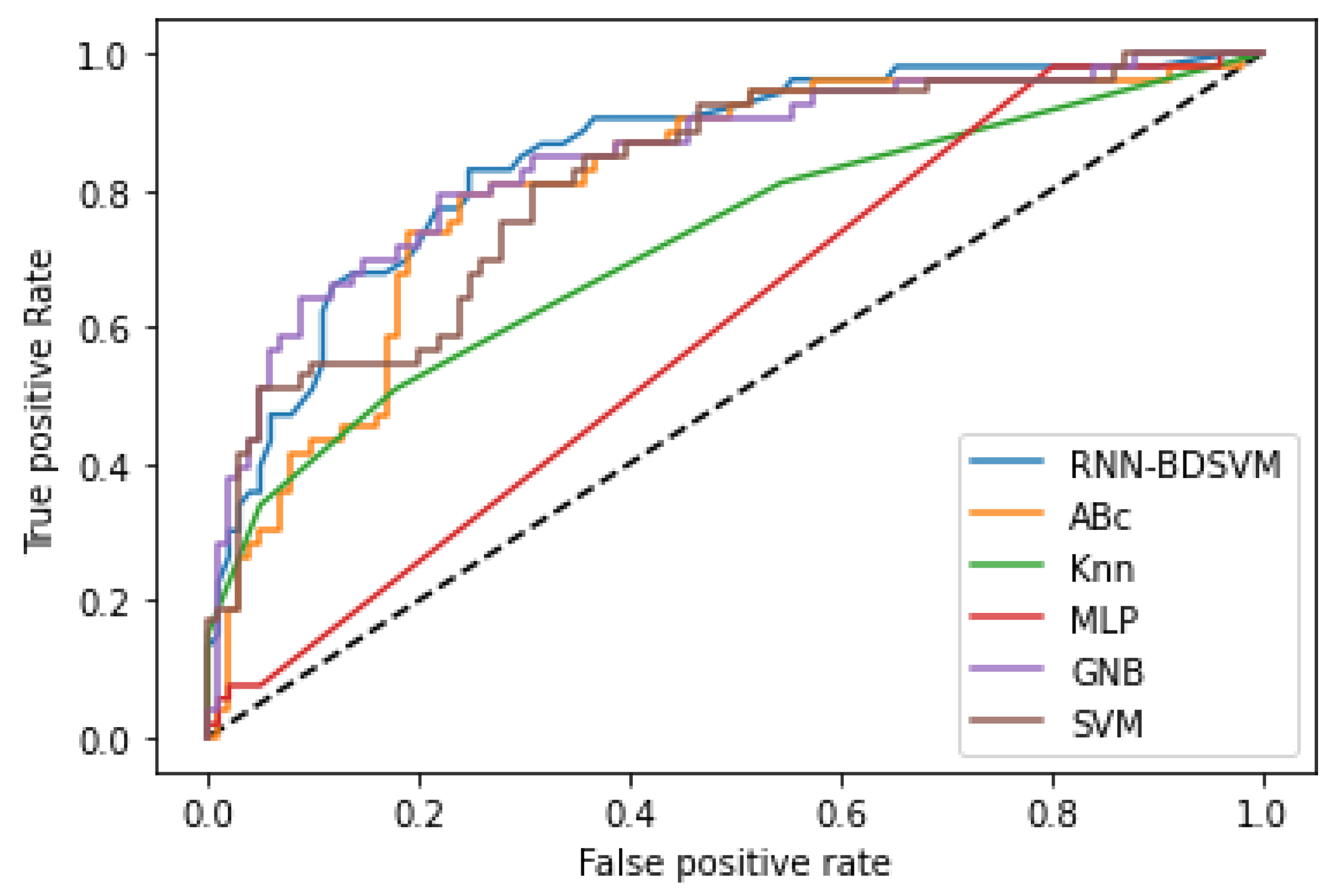
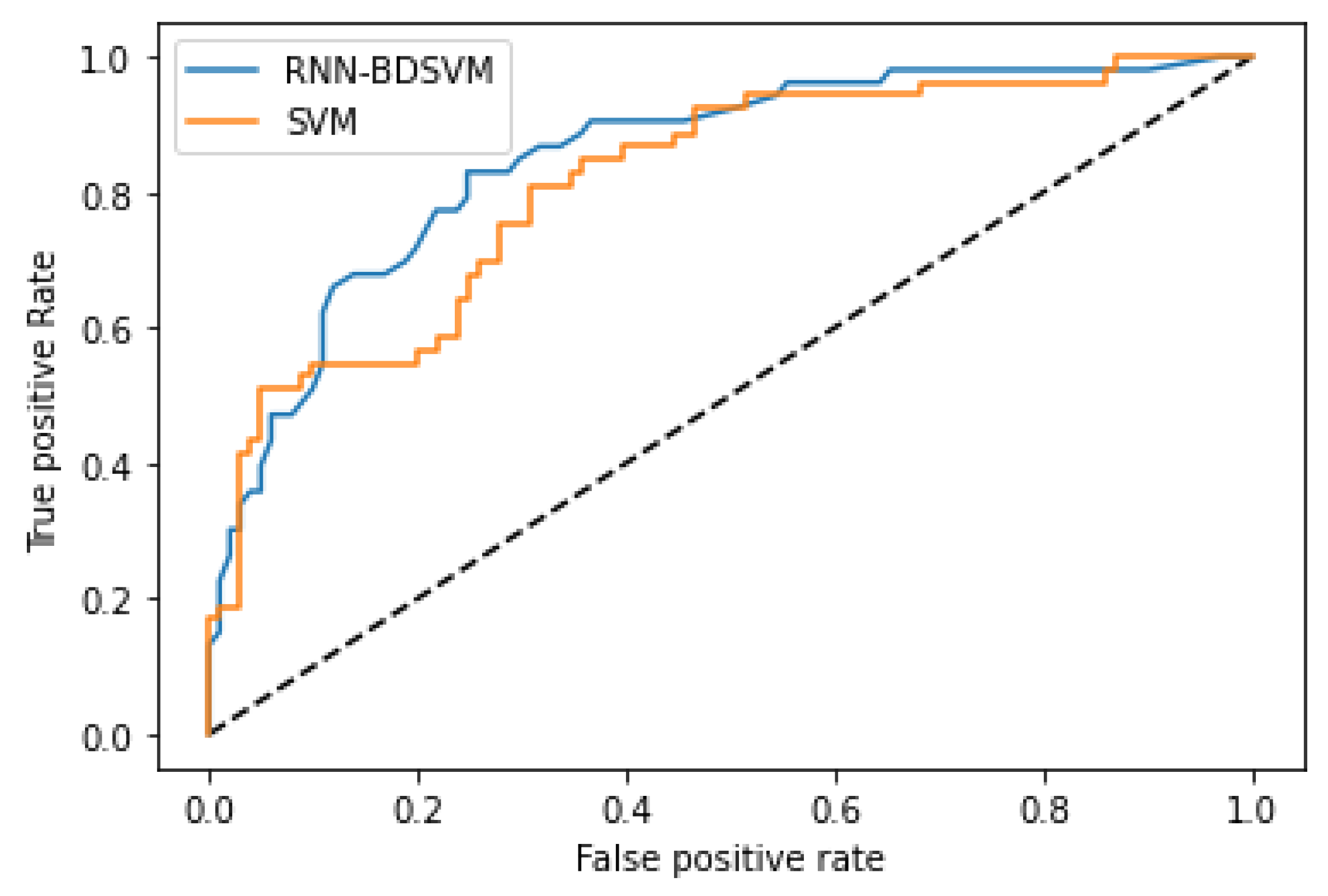
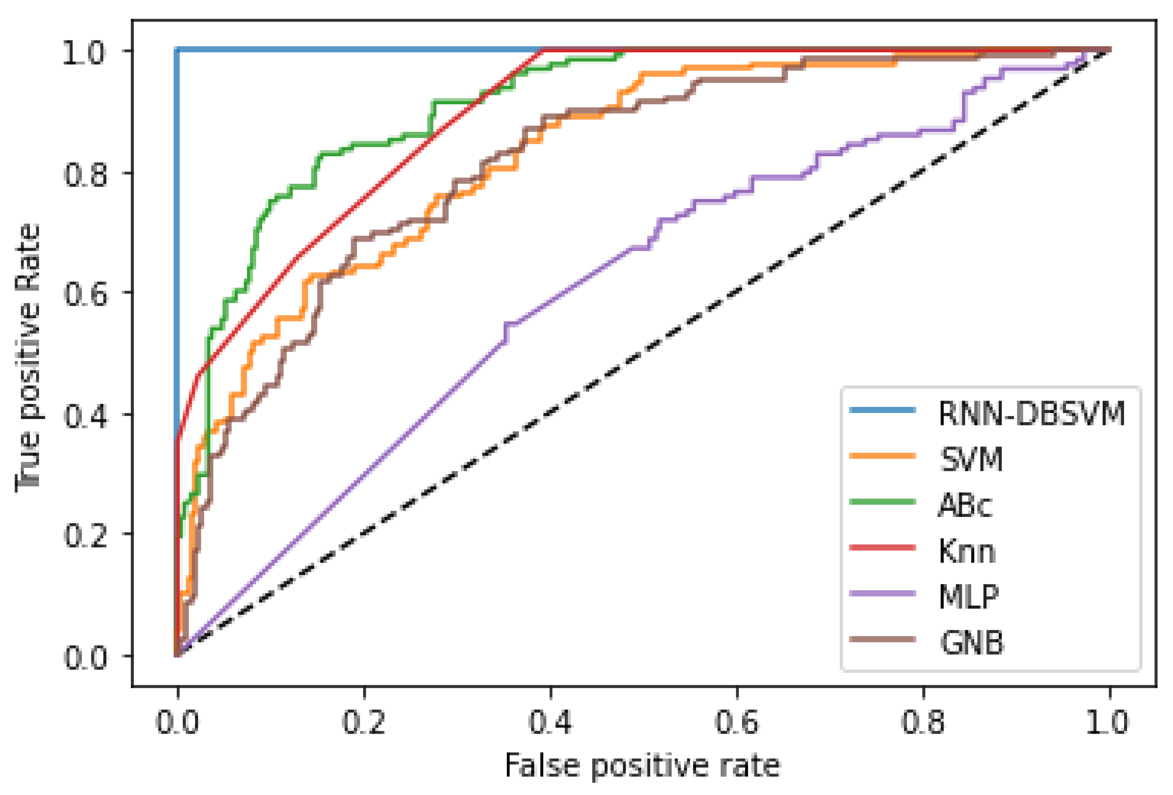
Additional comparison studies were performed on the PIMA and Germany Diabetes datasets and the ROC curves were used to calculate the AUC for the best performance obtained from each non-kernel classifier. Figure A4 and Figure A6 show the comparison of the ROC curves of the classifiers DT, KNN, MLP, NB, etc., and the Opt-RNN-DBSVM method, evaluated on the PIMA dataset. We point out that Opt-RNN-DBSVM quickly converges to the best results and obtains more true positives and a smaller number of false positives compared to several other classification methods.

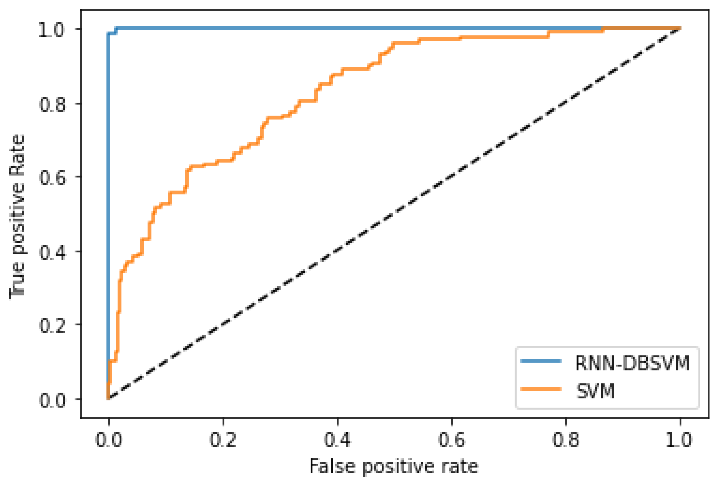
More comparisons are given in Appendix B; Figure A5 and Figure A7 show the comparison of the ROC curves of the classical SVM and Opt-RNN-DBSVM methods, evaluated on the Germany Diabetes dataset. More specifically, considering the performance measures “false positive rate” and “true positive rate”, predictions based on support vectors produced by Opt-RNN-DBSVM dominate predictions based on support vectors produced by other non-kernel classifiers.

6. Conclusions

The main challenges of SVM implementation are the number of local minima and the amount of computer memory required to solve the dual-SVM, which increase exponentially with respect to the size of the dataset. The Kernel-Adatron family of algorithms, ISDA and SMO, has handled very large classification and regression problems. However, these methods treat noise, boundary, and kernel samples in the same way, resulting in a blind search in unpromising areas. In this paper, we have introduced a hybrid approach to deal with these drawbacks, namely Optimal Recurrent Neural Network and Density-Based Support Vector Machine (Opt-RNN-DBSVM), which performs in six phases: the characterization of different samples, the elimination of samples having a weak probability of being support vectors, building an appropriate recurrent neural network based on an original energy function, and solving the differential equation system governing the RNN dynamics, using the Euler–Cauchy method implementing an optimal time step. Data preprocessing reduces the number of local minima in the dual-SVM; this reduction enables real-time decision making in big data problems. The RNN’s recurring architecture avoids the need to explore recently visited areas; this is an implicit tabu search. With the optimal time step, the search moves from the current vectors to the best neighboring support vectors. On one hand, two main, interesting fundamental results were demonstrated: the convergence of RNN-SVM to feasible solutions and the fact that Opt-RNN-DBSVM has very low time complexity compared to Const-RNN-SVM, SMO-SVM, ISDA-SVM, and L1QP-SVM. On the other hand, several experimental studies were conducted based on well-known datasets (IRIS, ABALONE, WINE, ECOLI, BALANCE, LIVER, SPECT, SEED, PIMA). Based on popular performance measures (accuracy, F1-score, precision, recall), Opt-RNN-DBSVM outperformed Const-RNN-SVM, KA-SVM, and some non-kernel models (cited in Table A1). In fact, Opt-RNN-DBSVM improved the accuracy by up to 3.43%, F1-score by up to 2.31%, precision by up to 7.52%, and recall by up to 6.5%. In addition, compared to SMO-SVM, ISDA-SVM, and L1QP-SVM, Opt-RNN-DBSVM provides a reduction in the number of support vectors by up to 32%, which permits us to save memory for large applications that implement several machine learning models. The main problem encountered in the implementation of Opt-RNN-DBSVM is the determination of the Lagrange parameters involved in the SVM energy function. In this sense, a genetic strategy will be introduced to determine these parameters considering each dataset. In future work, extensions of this method may include combining Opt-RNN-DBSVM with big data technologies to accelerate classification tasks on big data and introducing hybrid versions based on Opt-RNN, deep learning, and fuzzy-SVM.