Dynamical Analysis of an Age-Structured SVEIR Model with Imperfect Vaccine

Abstract

Based on the spread of COVID-19, in the present paper, an imperfectly vaccinated SVEIR model for latent age is proposed. At first, the equilibrium points and the basic reproduction number of the model are calculated. Then, we discuss the asymptotic smoothness and uniform persistence of the semiflow generated by the solutions of the system and the existence of an attractor. Moreover, LaSalle’s invariance principle and Volterra type Lyapunov functions are used to prove the global asymptotic stability of both the disease-free equilibrium and the endemic equilibrium of the model. The conclusion is that if the basic reproduction number $R_{\rho }$ is less than one, the disease will gradually disappear. However, if the number is greater than one, the disease will become endemic and persist. In addition, numerical simulations are also carried out to verify the result. Finally, suggestions are made on the measures to control the ongoing transmission of COVID-19.

1. Introduction

Since the proposal of compartmental models and epidemiological theories [1], an increasing number of scholars have applied them in the study of the transmission of epidemics. It is feasible to incorporate the latent period and vaccination strategy into the basic SIR model to establish SVEIR models. Recently, SVEIR models have been extensively studied.

For instance, Li et al. [2] discussed infectious diseases models considering incubation and vaccination periods and permanent immunity following recovery. The results achieved by [3] showed that if the probability of infection in a person was negligible when or before he/she became vaccinated, the disease could be successfully eliminated. This study also warned against overestimating the effectiveness of vaccination. Upadhyay et al. [4] simulated a computer virus model and found that the reinfection rate $\alpha$ was crucial in accurately describing the dynamics of the virus, and that the rate of infection could be reduced by increasing the number of susceptible nodes. Zhang et al. [5] constructed an SVEIR model with two time delays and analyzed the impact of these delay parameters on the system’s dynamic behavior. In addition, several SVEIR models have been developed to assess the influence of incomplete vaccination on epidemics, such as tuberculosis vaccine [6], hepatitis B vaccine [7], SARS vaccine [8], and HIV vaccine [9].

In recent years, many researchers have analyzed the impact of age on the transmission of epidemics. As a result, a number of age-structured epidemic models have been established, and significant progress has been made.

Specifically, Röst [10] built an SEIR model with age-affected infected individuals and discussed the stability of equilibria. Their results demonstrated that $k\left(a\right)$ had a direct impact on the value of $R_0$. Griffiths et al. [11] found that HIV was the most prevalent among individuals aged 20–29, and HIV prevention activities were the most effective in individuals under the age of 35. Magal et al. [12] concluded that if the infectious period coincided with the asymptomatic period for even one day, a complete eradication of the disease was not possible, even with quarantine measures in place. The analysis results in [13] suggested that to reduce the ratio of vector density to host density was the most effective method to suppress vector diffusion. Moreover, a smaller ratio indicated a smaller possibility of backward bifurcation and a lower basic reproduction ratio. Ebenman [14] explained that when density dependence was primarily influenced by young populations, stabilization could be achieved through increased competition between young and old populations. Species of different ages with greater ecological isolation were expected to be more stable. According to the study by [15], tuberculosis (TB) spread could be better controlled by reducing the TB spread coefficient $\beta$ and the TB infectiousness coefficient $\beta \rho$ in individuals undergoing treatment. As reported by Xu et al. [16,17], the conversion rate in the model was age-dependent, and both the conversion rate and the probability of the exposed patients to become infected increased with age. Dai and Zhang [18] claimed that the incidence of eating disorders could be lowered if people continued their education. Kenne et al. [19] demonstrated that birth rates directly affected the stability of diseases and that changing certain parameters triggered periodic epidemics, making it difficult to eradicate them from the population. Li and Wang [20] held that in order to effectively control infectious diseases, it was crucial to recruit few susceptible people, restrict travel, and ban large gatherings of people, in addition to vaccination. In the study by Wang et al. [21], age was reported to be an important factor directly affecting the outbreak time and spread speed of AIDS. In addition to the works mentioned above, more age-structured models have been discussed [22,23,24,25].

The rest of the paper is organized as follows. Section 2 presents an age-structured model, illustrates the existence and uniqueness of equilibrium points, and defines the basic reproduction number of the model. Section 3 studies the asymptotic smoothness and uniform persistence of the semiflow and demonstrates the existence of a global attractor. Section 4 analyzes the global stability of equilibrium states. Section 5 presents simulations for appropriate parameter values. Section 6 draws conclusions and discusses the results.

2. Mathematical Model and Existence of Equilibrium Points

In this section, a COVID-19 model in which the latent period depends on age is established. Additionally, the existence of equilibrium states is demonstrated, and the basic reproduction number of the model is calculated.

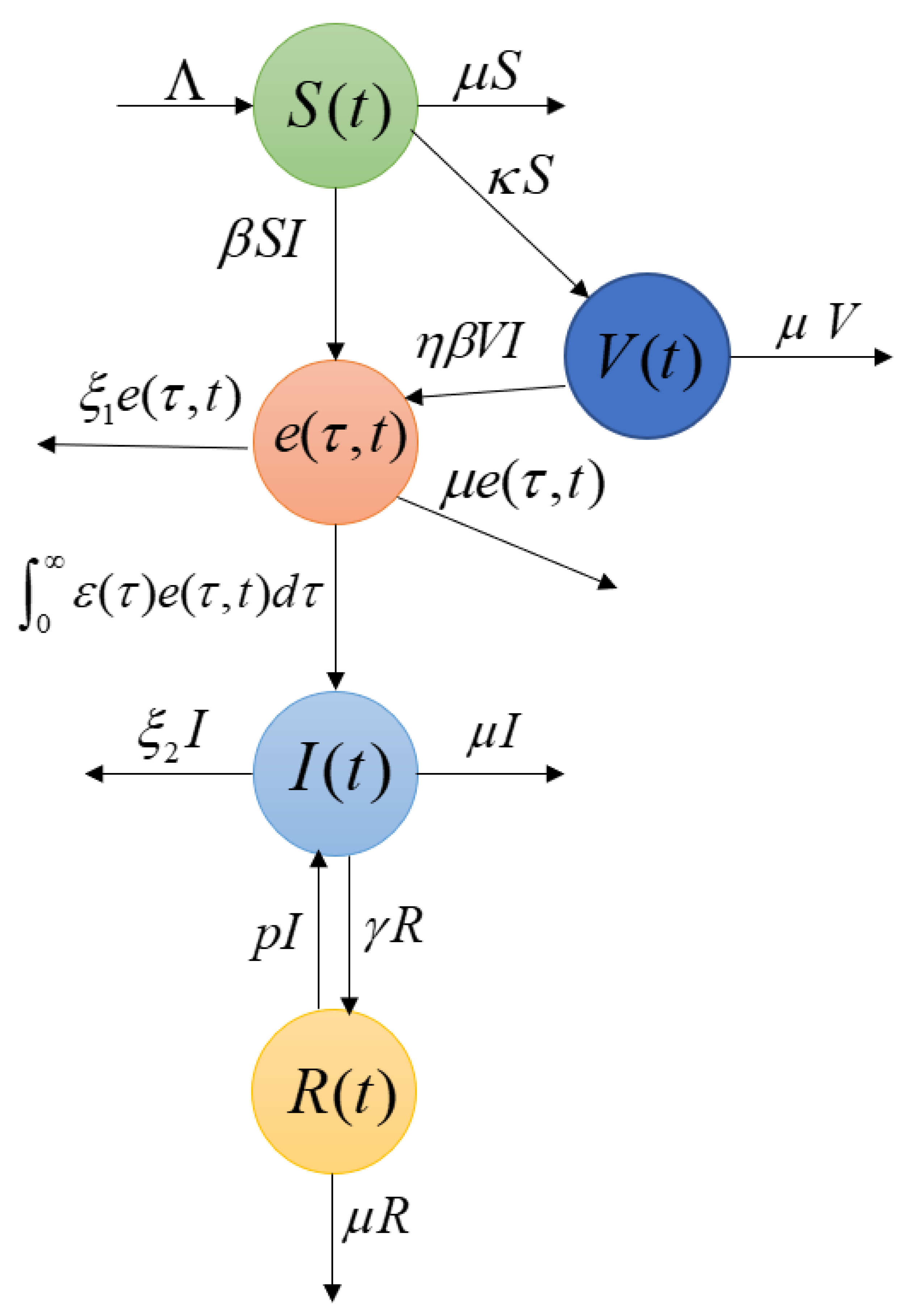
2.1. Mathematical Model

The population is subdivided into five subsets, namely, susceptible, vaccinated, exposed, infected, and recovered. The densities of susceptible individuals, vaccinated individuals, infected individuals, and recovered individuals at time t are represented by $S\left(t\right)$, $V\left(t\right)$, $I\left(t\right)$, and $R\left(t\right)$, respectively. The density of exposed individuals aged $\tau$ at time t is denoted by $e(\tau ,t)$. If a recovered person comes into contact with an infected person, there is a possibility that he or she will relapse and be involved in the transmission process. Even to a lesser degree, vaccinated individuals are assumed to be susceptible. Suppose that $\mathsf{\Lambda }$ is the recruitment rate of susceptible individuals and their vaccination rate is $\kappa$. $\eta \in (0,1)$ indicates the probability of COVID-19 infection in vaccinated individuals. $\beta$ is used to express the contact rate between infected individuals and individuals with susceptibility. Exposed individuals can become infected at an age-dependent rate of $\epsilon \left(\tau \right)$. p and $\gamma$ represent the reinfection rate of the recovered class and the recovery rate of the infected class, respectively. The mortality associated with the latency of the epidemic is ${\xi }_1$ and the epidemic-related mortality in the infected individuals is ${\xi }_2$. $\mu$ is the natural mortality rate of the populations. The interactions between state variables are illustrated in Figure 1.

The dynamics of state variables are characterized by the differential equations below:

$$\left\{\begin{array}{c}{S}^{{}^{\prime }}=\mathsf{\Lambda }-\beta SI-(\mu +\kappa )S,\hfill \\ V^{{}^{\prime }}=\kappa S-\eta \beta VI-\mu V,\hfill \\ e_{\tau }(\tau ,t)+e_t(\tau ,t)=-(\epsilon \left(\tau \right)+{\xi }_1+\mu )e(\tau ,t),\hfill \\ I^{{}^{\prime }}={\int }_0^{\infty }\epsilon \left(\tau \right)e(\tau ,t)d\tau -({\xi }_2+p+\mu )I+\gamma R,\hfill \\ R^{{}^{\prime }}=pI-(\gamma +\mu )R,\hfill \end{array}\right.$$

(1)

which is subject to the following boundary:

$$e\left|{}_{\tau =0}\right.=\beta SI+\eta \beta VI,$$

(2)

and the following initial conditions:

$$S\left|{}_{t=0}\right.=S_0,V\left|{}_{t=0}\right.=V_0,e\left|{}_{t=0}\right.=e_0\left(\tau \right),I\left|{}_{t=0}\right.=I_0,R\left|{}_{t=0}\right.=R_0,\forall \tau \ge 0,$$

(3)

and $S_0,V_0,I_0,R_0\in {\mathit{R}}_{+}$, $e_0\left(\tau \right)\in {\mathit{L}}_{+}^1(0,\infty )$.

To facilitate the calculation, we use:

$$\sigma \left(\tau \right)=\mu +{\xi }_1+\epsilon \left(\tau \right),\pi \left(\tau \right)=e^{-{\int }_0^{\tau }(\mu +{\xi }_1+\epsilon \left(s\right))ds},\theta ={\int }_0^{\infty }\epsilon \left(\tau \right)\pi \left(\tau \right)d\tau ,\forall \tau \ge 0.$$

(4)

2.2. Existence of Equilibrium Points

Firstly, through simple calculations, the disease-free equilibrium state of System (1) is obtained: $\ddot{G}=(\frac{\mathsf{\Lambda }}{\mu +\kappa },\frac{\kappa \mathsf{\Lambda }}{\mu (\mu +\kappa )},0,0,0)$. We define:

$$\frac{\mathsf{\Lambda }}{\mu +\kappa }:=\ddot{S},\frac{\kappa \mathsf{\Lambda }}{\mu (\mu +\kappa )}:=\ddot{V}.$$

(5)

Furthermore, assuming that $\widehat{G}=(\widehat{S},\widehat{V},\widehat{e}(·),\widehat{I},\widehat{R})$ is the steady-state solution of (1), $\widehat{G}$ satisfies:

$$\left\{\begin{array}{c}0=\mathsf{\Lambda }-\mu \widehat{S}-\kappa \widehat{S}-\beta \widehat{S}\widehat{I},\hfill \\ 0=\kappa \widehat{S}-\mu \widehat{V}-\eta \beta \widehat{V}\widehat{I},\hfill \\ {\widehat{e}}_{\tau }\left(\tau \right)=-\sigma \left(\tau \right)\widehat{e}\left(\tau \right),\hfill \\ 0={\int }_0^{\infty }\epsilon \left(\tau \right)\widehat{e}\left(\tau \right)d\tau -(\mu +{\xi }_2+p)\widehat{I}+\gamma \widehat{R},\hfill \\ 0=p\widehat{I}+(\mu +\gamma )\widehat{R},\hfill \\ \widehat{e}\left|{}_{t=0}\right.=(\beta \widehat{S}+\eta \beta \widehat{V})\widehat{I}.\hfill \end{array}\right.$$

(6)

Based on [26], the basic reproduction number $R_{\rho }$ is calculated with:

$$R_{\rho }=\frac{\beta \ddot{S}\theta +\eta \beta \ddot{V}\theta }{(\mu +{\xi }_2+p)-p\gamma /(\mu +\gamma )},$$

(7)

which refers to the average number of new infections generated by a single newly infected individual during the entire infectious period.

By integrating the third equation in (6) from 0 to $\tau$, we have:

$$\widehat{e}\left(\tau \right)=(\beta \widehat{S}+\eta \beta \widehat{V})\widehat{I}{e}^{-{\int }_0^{\tau }\sigma \left(s\right)ds}=(\beta \widehat{S}+\eta \beta \widehat{V})\widehat{I}\pi \left(\tau \right).$$

(8)

The first and second equations in (6) are solved and the results are:

$$\left\{\begin{array}{c}\widehat{S}=\frac{\mathsf{\Lambda }}{\mu +\kappa +\beta \widehat{I}},\hfill \\ \widehat{V}=\frac{\kappa \mathsf{\Lambda }}{(\mu +\eta \beta \widehat{I})(\mu +\kappa +\beta \widehat{I})},\hfill \\ \widehat{R}=\frac{p\widehat{I}}{\mu +\gamma }.\hfill \end{array}\right.$$

(9)

By substituting (7) and (8) into (5), we have:

$$h_0{\left(\widehat{I}\right)}^2+h_1\widehat{I}+h_2=0,$$

where

$$\left\{\begin{array}{c}{h}_0=\eta {\beta }^2[(\mu +p+{\xi }_2)(\mu +\gamma )-p\gamma ],\hfill \\ h_1=[(\mu +p+{\xi }_2)(\mu +\gamma )-p\gamma ][(\mu +\kappa )\eta \beta +\mu \beta ]-\eta {\beta }^2\mathsf{\Lambda }\theta (\mu +\gamma ),\hfill \\ h_2=[(\mu +p+{\xi }_2)(\mu +\gamma )-p\gamma ]\left[\mu (\mu +\gamma )\right]-\beta \mathsf{\Lambda }(\mu +\kappa \eta )(\mu +\gamma )\theta .\hfill \end{array}\right.$$

Let

$$T\left(\widehat{I}\right)=h_0{\left(\widehat{I}\right)}^2+h_1\widehat{I}+h_2.$$

It is evident that $h_0>0$, so we find that $T\left(\widehat{I}\right)\to \infty$ when $\widehat{I}\to \infty$.

$$\begin{array}{cc}\hfill T\left(0\right)& =h_2=[(\mu +p+{\xi }_2)(\mu +\gamma )-p\gamma ]\left[\mu (\mu +\gamma )\right]-\beta \mathsf{\Lambda }(\mu +\kappa \eta )(\mu +\gamma )\theta \hfill \\ \hfill & =\beta \mathsf{\Lambda }\theta (\mu +\gamma )(\mu +\kappa \eta )\left(\frac{1}{R_{\rho }}-1\right).\hfill \end{array}$$

(10)

Obviously, $T\left(0\right)<0$ when $R_{\rho }>1$. As $T\left(\widehat{I}\right)\in (0,\infty )$ is monotonically increasing, $T\left(\widehat{I}\right)=0$ has only one positive root $\widehat{I}$.

3. Preliminary Results

This section discusses some results about the semiflow generated by (1), such as its asymptotic smoothness and uniform persistence.

3.1. Semi-Flow

The characteristic method is used to seek the solution to the third equation in (1):

$$e(\tau ,t)=\left\{\begin{array}{c}{e}_0(\tau -t)\frac{\pi \left(\tau \right)}{\pi (\tau -t)},\tau \ge t\ge 0,\hfill \\ \beta S(t-\tau )+\eta \beta V(t-\tau )\left]I\right(t-\tau \left)\pi \right(\tau ),t>\tau \ge 0.\hfill \end{array}\right.$$

(11)

The following assumptions are made at first, and the state space of System (1) is defined later.

Assumption 1.

We make the following hypotheses:

(a) 

$\epsilon \left(\tau \right)\in {\mathit{L}}_{+}^1(0,\infty )$ and $\overline{\epsilon }=\underset{\tau \in [0,\infty )}{ess.sup}\epsilon \left(\tau \right)<\infty$;

(b) 

$\epsilon \left(\tau \right)$ is Lipschitz continuous on ${\mathit{R}}^{+}$, that is, $\forall m,v\in \epsilon \left(\tau \right)$, $\left|\epsilon \left(m\right)-\epsilon \left(v\right)\right|\le M_{\epsilon }\left|m-v\right|$;

(c) 

There is a ${\mu }_0$ belonging to $(0,\mu ]$ such that $\epsilon \left(\tau \right)\ge {\mu }_0$, $\forall \tau \ge 0$.

Let the state space of (1) be:

$$\mathbf{\Omega }=\left\{S\left(t\right),V\left(t\right),e(·,t),I\left(t\right),R\left(t\right)\in \mathbf{\Sigma }\left|S\left(t\right)+V\left(t\right)+{\int }_0^{\infty }e(\tau ,t)d\tau +I\left(t\right)+R\left(t\right)\le \frac{\mathsf{\Lambda }}{\mu }\right.\right\}.$$

The function space of (1) is defined as:

$$\mathbf{\Sigma }={\mathit{R}}_{+}^2\times {\mathit{L}}_{+}^1(0,\infty )\times {\mathit{R}}_{+}^2,$$

the norm is represented as:

$${∥(x_1,x_2,x_3,x_4,x_5)∥}_{\mathbf{\Sigma }}=\left|x_1\right|+\left|x_2\right|+{\int }_0^{\infty }\left|x_3\left(\tau \right)\right|d\tau +\left|x_4\right|+\left|x_5\right|,$$

(12)

and the initial condition is:

$$x_0=(S_0,V_0,e_0(·),I_0,R_0)\in \mathbf{\Sigma }.$$

(13)

According to [27], System (1) has a unique non-negative solution. Thus, the semiflow generated by (1) is acquired:

$$\Psi \left(t\right)x_0=(S\left(t\right),V\left(t\right),e(·,t),I\left(t\right),R\left(t\right)),fort\ge 0,x_0\in \mathbf{\Sigma },$$

and the norm is similar to (12).

Proposition 1.

For System (1), we have

(a) 

$\forall t\ge 0$, for each $x_0\in \mathbf{\Omega }$, we have $\Psi \left(t\right)x_0\in \mathbf{\Omega }$;

(b) 

Ω attracts all points in Σ, and Ψ is point-dissipative.

Proof. 

Since $\pi \left(0\right)=1$ and $\frac{d}{d\tau }\pi \left(\tau \right)=-\sigma \left(\tau \right)\pi \left(\tau \right)$, the variation of the constant formula, we obtain:

$${∥\Psi \left(t\right)x_0∥}_{\mathbf{\Sigma }}\le \frac{\mathsf{\Lambda }}{\mu }-exp(-\mu t)·\left(\frac{\mathsf{\Lambda }}{\mu }-{∥x_0∥}_{\mathbf{\Sigma }}\right),\forall t\ge 0.$$

(14)

It means that $\Psi \left(t\right)x_0\in \mathbf{\Omega }$ for any solution of (1) satisfying $x_0\in \mathbf{\Omega }$, $\forall t\ge 0$. Moreover, based on (14), ${\displaystyle \underset{t\to \infty }{lim}}∥\Psi \left(t\right)x_0∥\le \mathsf{\Lambda }/\mu$, $\forall x_0\in \mathbf{\Sigma }$. As a result, $\mathbf{\Omega }\subseteq \mathbf{\Sigma }$ attracts all points and $\Psi$ is point-dissipative. This proposition is proved valid. □

According to Assumption 1 and Proposition 1, the following proposition is made.

Proposition 2.

There exists $M\ge \frac{\mathsf{\Lambda }}{\mu }$, and if $x_0\in \mathbf{\Sigma }$ and ${∥x_0∥}_{\mathbf{\Sigma }}\le M$, then for all $t\ge 0$, we have:

(a) 

$S\left(t\right),V\left(t\right),{\int }_0^{\infty }e(\tau ,t)d\tau ,I\left(t\right),R\left(t\right)\in [0,M]$;

(b) 

$e(0,t)\le \beta (1+\eta )M^2$.

3.2. Asymptotic Smoothness

In order to explore the global properties of the semiflow, it is essential to study the asymptotic smoothness of the semiflow ${\left\{\Psi \left(t\right)x_0\right\}}_{t\ge 0}$.

Definition 1

([28]). For any nonempty closed bounded set $\mathit{Z}\subset \mathbf{\Sigma }$ in which $\Psi \left(t\right)\mathit{Z}\subset \mathit{Z}$, if there is a compact set ${\mathit{Z}}_0\subset \mathit{Z}$ such that ${\mathit{Z}}_0$ attracts $\mathit{Z}$, then $\Psi \left(t\right)x_0:{\mathit{R}}_{+}\times \mathbf{\Sigma }\to \mathbf{\Sigma }$ is asymptotically smooth.

Lemma 1

([28]). If the following cases are met:

(a) 

There is a continuous function $u:{\mathit{R}}_{+}\times {\mathit{R}}_{+}\to {\mathit{R}}_{+}$ such that ${\displaystyle \underset{t\to \infty }{lim}}u(c,t)=0$ and ${∥x_0∥}_{\mathbf{\Sigma }}\le h$, ${∥{\phi }_1\left(t\right)x_0∥}_{\mathbf{\Sigma }}\le u(c,t)$;

(b) 

${\phi }_2\left(t\right)x_0$ is fully continuous, where t is non-negative;

then, $\Psi \left(t\right)x_0={\phi }_1\left(t\right)x_0+{\phi }_2\left(t\right)x_0:{\mathit{R}}_{+}\times \mathbf{\Sigma }\to \mathbf{\Sigma }$ is asymptotically smooth in Σ.

Here, we divide $\Psi \left(t\right)x_0$ into two operators as follows:

$${\phi }_1\left(t\right)x_0=(0,0,f_3(·,t),0,0),{\phi }_2\left(t\right)x_0=(S\left(t\right),V\left(t\right),{\stackrel{⌣}{f}}_3(·,t),I\left(t\right),R\left(t\right)),$$

where $f_3(\tau ,t)$ and ${\stackrel{⌣}{f}}_3(\tau ,t)$ can be obtained by (6). It is evident that $\Psi \left(t\right)x_0={\phi }_1\left(t\right)x_0+{\phi }_2\left(t\right)x_0$, where t is non-negative. To prove (a) in Lemma 1, we need to first verify the following proposition.

Proposition 3.

Let $u(c,t)=c{e}^{-(\mu +{\mu }_0)t}$, where $c>0$. Then, ${\displaystyle \underset{t\to \infty }{lim}}u(c,t)=0$, and if ${∥x_0∥}_{\mathbf{\Sigma }}\le c$, ${∥{\phi }_1\left(t\right)x_0∥}_{\mathbf{\Sigma }}\le u(c,t)$.

Proof. 

Obviously, $u(c,t)$ approaches 0 if $t\to \infty$. According to (6), we know:

$$y_3(\tau ,t)=\left\{\begin{array}{c}{e}_0(\tau -t)\frac{\pi \left(\tau \right)}{\pi (\tau -t)},\tau \ge t\ge 0,\hfill \\ 0,t>\tau \ge 0.\hfill \end{array}\right.$$

(15)

For $x_0\in \mathbf{\Omega }$ and ${∥x_0∥}_{\mathbf{\Sigma }}\le c$, we have:

$$\begin{array}{cc}\hfill & {∥{\phi }_1\left(t\right)x_0∥}_{\mathbf{\Sigma }}=\left|0\right|+\left|0\right|+{\int }_0^{\infty }\left|y_3(a,t)\right|da+\left|0\right|+\left|0\right|\hfill \\ \hfill & ={\int }_0^{\infty }\left|e_0\left(\tau \right)\frac{\pi (t+\tau )}{\pi \left(\tau \right)}\right|d\tau \hfill \\ \hfill & ={\int }_0^{\infty }\left|e_0\left(\tau \right)exp\left(-{\int }_{\tau }^{t+\tau }\sigma \left(s\right)ds\right)\right|d\tau .\hfill \end{array}$$

(16)

Note that $\sigma \left(\tau \right)\ge {\mu }_0+\mu +{\xi }_1$, $\forall \tau \ge 0$ holds true, and it is easy to obtain:

$${∥{\phi }_1\left(t\right)x_0∥}_{\mathbf{\Sigma }}\le c{e}^{-(\mu +{\mu }_0)t}.$$

(17)

This proposition is proved true. □

Since ${\mathit{L}}_{+}^1(0,\infty )$ is an integral part of $\mathbf{\Sigma }$, we need a compactness concept in ${\mathit{L}}_{+}^1(0,\infty )$. Subsequently, we verify (b) in Lemma 1.

Based on [29] and the conclusion of Proposition 3, ${\stackrel{⌣}{y}}_3(\tau ,t)$ remains in a precompact subset of ${\mathit{L}}_{+}^1(0,\infty )$, which is independent of $x_0\in \mathbf{\Omega }$. According to (11), we have:

$$0\le {\stackrel{⌣}{f}}_3(\tau ,t)=\left\{\begin{array}{c}0,\tau \ge t\ge 0,\hfill \\ \beta S(t-\tau )+\eta \beta V(t-\tau )\left]I\right(t-\tau \left)\pi \right(\tau ),t>\tau \ge 0.\hfill \end{array}\right.$$

(18)

As $\pi \left(\tau \right)=e^{-{\int }_0^{\tau }\sigma \left(s\right)ds}\le e^{-({\mu }_0+\mu +{\xi }_1)\tau }$, ${\stackrel{⌣}{f}}_3(\tau ,t)\le \beta (1+\eta )M^2{e}^{-({\mu }_0+\mu +{\xi }_1)\tau }$ can be derived from (a) in Proposition 2. This result implies that the condition for the bounded closed set presented in [29] is met. There is a small enough $c\in (0,t)$ such that:

$$\begin{array}{cc}\hfill & {\int }_0^{\infty }\left|{\stackrel{⌣}{f}}_3(\tau +c,t)-{\stackrel{⌣}{f}}_3(\tau ,t)\right|da={\int }_0^t\left|e(\tau +c,t)-e(\tau ,t)\right|d\tau \hfill \\ \hfill & \le {\int }_0^{t-c}e(0,t-\tau -c)\left|\pi (\tau +c)-\pi \left(\tau \right)\right|d\tau \hfill \\ \hfill & +{\int }_{t-c}^t\left|e(0,t-\tau )\pi \left(\tau \right)\right|d\tau \hfill \\ \hfill & +{\int }_0^{t-c}\left|e(0,t-\tau -c)-e(0,t-\tau )\right|\pi \left(\tau \right)d\tau .\hfill \end{array}$$

We define:

$${\int }_0^{t-c}\left|e(0,t-\tau -c)-e(0,t-\tau )\right|\pi \left(\tau \right)d\tau :=\Delta .$$

Note that $0\le \pi \left(\tau \right)\le e^{-({\mu }_0+\mu +{\xi }_1)\tau }\le 1$, and we obtain:

$$\begin{array}{cc}\hfill & {\int }_0^{t-c}\left|\pi (\tau +c)-\pi \left(\tau \right)\right|d\tau ={\int }_0^{t-c}\pi \left(\tau \right)d\tau -{\int }_c^t\pi \left(\tau \right)d\tau \hfill \\ \hfill & ={\int }_0^{t-c}\pi \left(\tau \right)d\tau -{\int }_c^{t-c}\pi \left(\tau \right)d\tau -{\int }_{t-c}^t\pi \left(\tau \right)d\tau \hfill \\ \hfill & ={\int }_0^c\pi \left(\tau \right)d\tau -{\int }_{t-c}^t\pi \left(\tau \right)d\tau \le c.\hfill \end{array}$$

Hence, according to (b) in Proposition 2, we obtain:

$${\int }_0^{\infty }\left|{\stackrel{⌣}{f}}_3(\tau +c,t)-{\stackrel{⌣}{f}}_3(\tau ,t)\right|d\tau \le 2\beta (1+\eta )M^{2}c+\Delta .$$

Combining (1) and Proposition 2, we have:

$$\left|\frac{dS}{dt}\right|\le \mathsf{\Lambda }+(\mu +\kappa )M+\beta M^2,$$

which indicates that $\left|\frac{dS}{dt}\right|$ is bounded by $K_S=\beta M^2+(\mu +\kappa )M+\mathsf{\Lambda }$ and $S\left(t\right)\in [0,\infty )$ is Lipschitz continuous with a coefficient $K_S$. $\left|\frac{dV}{dt}\right|$ is bounded by $K_V=-\eta \beta M^2+(\mu +\kappa )M$, and $V\left(t\right)\in [0,\infty )$ is also Lipschitz continuous with a Lipschitz coefficient $K_V$. Likewise, it can also be deduced from the fourth equation in (1) and Assumption 1 that $\left|\frac{dI}{dt}\right|\le (\mu +{\xi }_2+p)M+\gamma M+\overline{\epsilon }M:=K_I$. It is easy to infer that $I\left(t\right)$ is Lipschitz continuous with a coefficient $K_I$. According to the lemma of Lipschitz continuity [30], $SI\in [0,\infty )$ is Lipschitz continuous with a coefficient $K_{SI}=(K_S+K_I)M$, and $VI\in [0,\infty )$ is also Lipschitz continuous with a coefficient $K_{VI}=(K_V+K_I)M$. Hence,

$$\Delta \le {\int }_0^{t-c}\beta (1+\eta )M(K_S+K_V+2K_I)c{e}^{-({\mu }_0+\mu )\tau }d\tau \le \frac{\beta (1+\eta )(K_{SI}+K_{VI})c}{{\mu }_0+\mu }.$$

Based on the above results, we obtain:

$${\int }_0^{\infty }\left|{\stackrel{⌣}{f}}_3(\tau +c,t)-{\stackrel{⌣}{f}}_3(\tau ,t)\right|d\tau \le \left[2\beta (1+\eta )M^2+\frac{\beta (1+\eta )(K_{SI}+K_{VI})}{{\mu }_0+\mu }\right]c.$$

Therefore, ${\displaystyle \underset{c\to 0}{lim}}{\int }_0^{\infty }\left|{\stackrel{⌣}{f}}_3(\tau +c,t)-{\stackrel{⌣}{f}}_3(\tau ,t)\right|d\tau =0$ is uniform for any $x_0\in \mathit{Z}$, and ${\stackrel{⌣}{f}}_3(\tau ,t)$ remains in a precompact subset ${\mathit{Z}}_{{\stackrel{⌣}{f}}_3}$ of ${\mathit{L}}_{+}^1(0,\infty )$. Moreover, ${\phi }_2\left(t\right)Z\subset [0,M]\times [0,M]\times {\mathit{Z}}_{{\stackrel{⌣}{f}}_3}\times [0,M]\times [0,M]$ is compact in $\mathbf{\Sigma }$. According to the lemma of the bounded and closed compact set [29], ${\phi }_2\left(t\right)x_0$ is fully continuous. Considering the above, Lemma 1 is proved true.

Two important theorems are acquired as follows.

Theorem 1.

${\left\{\Psi \left(t\right)x_0\right\}}_{t\ge 0}$ is asymptotically smooth.

Theorem 2.

${\left\{\Psi \left(t\right)x_0\right\}}_{t\ge 0}$ has a global attractor $\vartheta \in \mathbf{\Sigma }$, which attracts the bounded sets of Σ.

3.3. Uniform Persistence

Lemma 2

([17]). The scalar Volterra integro-differential equation

$$y_t=-hy\left(t\right)+{\int }_0^{\infty }c\left(\alpha \right)y(t-\alpha )d\alpha ,y\left(0\right)>0,$$

where $c(·)\in L_{+}^1(0,\infty )$, $h>0$, and ${\int }_0^{\infty }c\left(\alpha \right)d\alpha >h$, has a unique unbounded solution $y\left(t\right)$.

We denote:

$$\overline{\tau }=inf\left\{\tau :{\int }_{\tau }^{\infty }\epsilon \left(\tau \right)d\tau =0\right\}$$

and define:

$$\stackrel{⌣}{\mathbf{\Sigma }}={\mathit{L}}_{+}^1(0,\infty )\times {\mathit{R}}_{+}^2,$$

$$\stackrel{⌣}{\mathit{B}}=\left\{{\left(e\right(·,t),I(t),R(t\left)\right)}^{{}^{\prime }}\in \stackrel{⌣}{\mathbf{\Sigma }}:{\int }_0^{\tau }e(\tau ,t)d\tau >0orI\left(t\right)>0orR\left(t\right)>0\right\}.$$

In addition, we make $\mathit{B}={\mathit{R}}_{+}^2\times \stackrel{⌣}{\mathit{B}},\partial \mathit{B}=\mathbf{\Sigma }\backslash \mathit{B},\partial \stackrel{⌣}{\mathit{B}}=\stackrel{⌣}{\mathbf{\Sigma }}\backslash \stackrel{⌣}{\mathit{B}}$, where $\mathit{B}$ and $\partial \mathit{B}$ are both positive sets. According to [31], several results can be reached. Before the analysis of the uniform persistence of the semiflow ${\left\{\Psi \left(t\right)x_0\right\}}_{t\ge 0}$, the following theorem should be proved true.

Theorem 3.

For the semiflow ${\left\{\Psi \left(t\right)x_0\right\}}_{t\ge 0}$ restricted to ∂B, the disease-free equilibrium $\ddot{G}$ of System (1) is globally asymptotically stable.

Proof. 

Let $(S_0,V_0,e_0\left(\tau \right),I_0,R_0)\in \partial \mathit{B}$, and we have $(e_0\left(\tau \right),I_0,R_0)\in \partial \stackrel{⌣}{\mathit{B}}$. Then, the following system is obtained:

$$\left\{\begin{array}{c}{e}_{\tau }(\tau ,t)+e_t(\tau ,t)=-(\mu +{\xi }_1+\epsilon \left(\tau \right))e(\tau ,t),\hfill \\ I^{{}^{\prime }}={\int }_0^{\infty }\epsilon \left(\tau \right)e(\tau ,t)d\tau -(\mu +{\xi }_2+p)I+\gamma R,\hfill \\ R^{{}^{\prime }}=pI-(\mu +\gamma )R,\hfill \end{array}\right.$$

(19)

which is subject to the boundary

$$e\left|{}_{\tau =0}\right.=(\beta S+\eta \beta V)I,$$

(20)

and the following initial conditions:

$$e\left|{}_{t=0}\right.=e_0\left(\tau \right),I\left|{}_{t=0}\right.=I_0,R\left|{}_{t=0}\right.=R_0.$$

(21)

As ${\displaystyle \underset{t\to \infty }{lim}}S\left(t\right)\le \frac{\mathsf{\Lambda }}{\mu }$ and ${\displaystyle \underset{t\to \infty }{lim}}V\left(t\right)\le \frac{\mathsf{\Lambda }}{\mu }$, according to the comparison principle, we obtain:

$$e(\tau ,t)\le \stackrel{⌣}{e}(\tau ,t),I\left(t\right)\le \stackrel{⌣}{I}\left(t\right),R\left(t\right)\le \stackrel{⌣}{R}\left(t\right),$$

(22)

where $(\stackrel{⌣}{e}(\tau ,t),\stackrel{⌣}{I}\left(t\right),\stackrel{⌣}{R}\left(t\right))$ satisfies:

$$\left\{\begin{array}{c}{\stackrel{⌣}{e}}_{\tau }(\tau ,t)+\stackrel{⌣}{e}(\tau ,t)=-(\mu +{\xi }_2+\epsilon \left(\tau \right))\stackrel{⌣}{e}(\tau ,t),\hfill \\ {\stackrel{⌣}{I}}^{{}^{\prime }}\left(t\right)={\int }_0^{\infty }\epsilon \left(\tau \right)\stackrel{⌣}{e}(\tau ,t)d\tau -(\mu +{\xi }_2+p)I+\gamma R,\hfill \\ {\stackrel{⌣}{R}}^{{}^{\prime }}\left(t\right)=p\stackrel{⌣}{I}\left(t\right)-(\mu +\gamma )\stackrel{⌣}{R}\left(t\right).\hfill \end{array}\right.$$

(23)

The boundary condition is:

$$\stackrel{⌣}{e}\left|{}_{\tau =0}\right.=\beta (1+\eta )\frac{\mathsf{\Lambda }}{\mu }\stackrel{⌣}{I}\left(t\right),$$

(24)

and the initial conditions are:

$$\stackrel{⌣}{e}\left|{}_{t=0}\right.=e_0\left(\tau \right),I\left|{}_{t=0}\right.=0,R\left|{}_{t=0}\right.=0.$$

(25)

Calculating the first equation in (25) in the same way as (11) and (12), we obtain:

$$\stackrel{⌣}{e}(\tau ,t)=\left\{\begin{array}{c}{\stackrel{⌣}{e}}_0(\tau -t)\frac{\pi \left(\tau \right)}{\pi (\tau -t)},\tau \ge t\ge 0,\hfill \\ \beta (1+\eta )\frac{\mathsf{\Lambda }}{\mu }\stackrel{⌣}{I}(t-\tau )\pi \left(\tau \right),t>\tau \ge 0.\hfill \end{array}\right.$$

(26)

Substituting (26) into the second equation in System (23), we can obtain:

$${\stackrel{⌣}{I}}^{{}^{\prime }}\left(t\right)=Q\left(t\right)+\beta (1+\eta )\frac{\mathsf{\Lambda }}{\mu }{\int }_0^t\epsilon \left(\tau \right)\pi \left(\tau \right)\stackrel{⌣}{I}(t-\tau )d\tau -(\mu +{\xi }_2+p)\stackrel{⌣}{I}\left(t\right)+\gamma \stackrel{⌣}{R}\left(t\right),$$

(27)

where

$$Q\left(t\right)={\int }_t^{\infty }\delta \left(\tau \right)e_0(\tau -t)\frac{\pi \left(\tau \right)}{\pi (\tau -t)}d\tau .$$

Since $(e_0\left(\tau \right),I_0,R_0)\in \partial \stackrel{⌣}{\mathit{B}}$, we have $Q\left(t\right)=0$, for $t\ge 0$. Thus, $\stackrel{⌣}{I}\left(t\right)=0$ is the only solution of the following equation:

$$\left\{\begin{array}{c}{\stackrel{⌣}{I}}^{{}^{\prime }}\left(t\right)=\beta (1+\eta )\frac{\mathsf{\Lambda }}{\mu }{\int }_0^t\epsilon \left(\tau \right)\pi \left(\tau \right)\stackrel{⌣}{I}(t-\tau )d\tau +\gamma R\left(t\right)-(\mu +{\xi }_2+p)\stackrel{⌣}{I}\left(t\right),\hfill \\ {\stackrel{⌣}{R}}^{{}^{\prime }}\left(t\right)=p\stackrel{⌣}{I}\left(t\right)-(\mu +\gamma )\stackrel{⌣}{R}\left(t\right),\hfill \end{array}\right.$$

(28)

and its initial conditions are:

$$\stackrel{⌣}{I}\left|{}_{t=0}\right.=I_0,\stackrel{⌣}{R}\left|{}_{t=0}\right.=R_0.$$

(29)

According to (26), for $0\le \tau <t$, we have $\stackrel{⌣}{e}(\tau ,t)=0$. When $\tau \ge t$, we have:

$${∥\stackrel{⌣}{e}(\tau ,t)∥}_{L^1}={\int }_t^{+\infty }{e}_0(\tau -t)\frac{\pi \left(\tau \right)}{\pi (\tau -t)}d\tau \le e^{-(\mu +{\mu }_0)t}{∥e_0(\tau -t)∥}_{L_{+}^1}.$$

Since $\underset{t\to 0}{lim}\stackrel{⌣}{e}(\tau ,t)=0$, ${\displaystyle \underset{t\to \infty }{lim}}e(\tau ,t)=0$. Furthermore, it can be deduced from System (1) that ${\displaystyle \underset{t\to \infty }{lim}}S\left(t\right)=\ddot{S}$, $\underset{t\to \infty }{lim}V\left(t\right)=\ddot{V}$. Thus, $\ddot{G}$ is globally asymptotically stable in $\partial \mathit{B}$. This theorem is proved valid. □

We now demonstrate the uniform persistence of ${\left\{\Psi \left(t\right)x_0\right\}}_{t\ge 0}$.

Theorem 4.

If $R_{\rho }>1$, then the semiflow ${\left\{\Psi \left(t\right)x_0\right\}}_{t\ge 0}$ is uniformly persistent with respect to $(\mathit{B},\partial \mathit{B})$. It means that there is a $\epsilon >0$ such that ${\displaystyle \underset{t\to \infty }{lim}}{∥\Psi \left(t\right)x_0∥}_{\mathbf{\Sigma }}\ge \epsilon$ for any $x_0\in \mathit{B}$. Furthermore, there is a compact global attractor ${\vartheta }_0\in \mathit{B}$ of ${\left\{\Psi \left(t\right)x_0\right\}}_{t\ge 0}$.

Proof. 

Based on Theorem 3, we only need to demonstrate that there exist $\overline{T}\ge 0$ and $\epsilon >0$ such that $\underset{t\to \infty }{lim}{∥\Psi \left(t\right)x_0∥}_{\mathbf{\Sigma }}\ge \epsilon$, $\forall x_0\in \mathit{B}$. The specific steps are as follows:

$$W^S\left(\ddot{G}\right)\cap B=⌀,$$

where

$$W^S\left(\ddot{G}\right)=\left\{x_0\in \mathit{B}:{\displaystyle \underset{t\to \infty }{lim}}\Psi \left(t\right)x_0=\ddot{G}\right\}.$$

On the contrary, we suppose that $\exists f_0\in \mathit{B}$ such that ${\displaystyle \underset{t\to \infty }{lim}}\Psi \left(t\right)f_0=\ddot{G}$. Then, for t non-negative, there is a sequence $\left\{f_n\right\}\subset \mathit{B}$ such that:

$${∥\Psi \left(t\right)f_n-\ddot{G}∥}_{\mathbf{\Sigma }}\le \frac{1}{n}.$$

We denote:

$$\Psi \left(t\right)f_n=(S_n\left(t\right),V_n\left(t\right),e_n(·,t),I_n\left(t\right),R_n\left(t\right)),$$

$$f_n=(S_n\left(0\right),V_n\left(0\right),e_n\left(0\right),I_n\left(0\right),R_n\left(0\right)).$$

Selecting a sufficiently big $n>0$ such that $\ddot{S}-\frac{1}{n}>0$, $\ddot{V}-\frac{1}{n}>0$, there is a positive $\overline{T}$ for it, and when $t>\overline{T}$, we have:

$$\begin{array}{cc}\hfill \ddot{S}-\frac{1}{n}<S_n\left(t\right)<& \ddot{S}+\frac{1}{n},\hfill \\ \hfill \ddot{V}-\frac{1}{n}<V_n\left(t\right)<& \ddot{V}+\frac{1}{n},\hfill \\ \hfill -\frac{1}{n}<I_n\left(t\right)<& \frac{1}{n},\hfill \\ \hfill -\frac{1}{n}<R_n\left(t\right)<& \frac{1}{n}.\hfill \end{array}$$

(30)

According to (11) and (12), we obtain:

$$e(\tau ,t)\ge \left[\beta S\right(t-\tau )+\eta \beta V(t-\tau \left)\right]I(t-\tau )\pi \left(\tau \right).$$

(31)

Combining (30) and (31) with the fourth equation in (1), we have:

$$I_n\left(t\right)\ge u_n\left(t\right)$$

where $u_n\left(t\right)$ satisfies:

$$\left\{\begin{array}{c}\frac{d{u}_n\left(t\right)}{dt}={\int }_0^{\infty }\beta \left[\left(\ddot{S}-\frac{1}{n}\right)+\eta \beta \left(\ddot{V}-\frac{1}{n}\right)\right]\epsilon \left(\tau \right)\pi \left(\tau \right)u_n(t-\tau )d\tau \hfill \\ +\gamma u_n\left(t\right)-(\mu +{\xi }_2+p)u_n\left(t\right),\hfill \\ u_n\left(t\right)=I_n\left|{}_{t=0}\right.\ge 0.\hfill \end{array}\right.$$

When $u_n\left(0\right)=0$, $u_n\left(t\right)>0$. To prevent the loss of generality, let $u_n\left(0\right)>0$. By $R_{\rho }>1$, we choose a large enough $n\in {\mathit{R}}_{+}$ to satisfy:

$$\frac{\left[\beta \left(\ddot{S}-\frac{1}{n}\right)+\eta \beta \left(\ddot{V}-\frac{1}{n}\right)\right](\mu +\gamma )\theta }{(\mu +{\xi }_2+p)(\mu +\gamma )-p\gamma }>1.$$

Then, we can deduce that:

$${\int }_0^{\tau }\left[\beta \left(\ddot{S}-\frac{1}{n}\right)+\eta \beta \left(\ddot{V}-\frac{1}{n}\right)\right]\epsilon \left(\tau \right)\pi \left(\tau \right)d\tau >(\mu +{\xi }_2+p)-\frac{p\gamma }{\mu +\gamma }.$$

It can be inferred from Lemma 2 that $u_n\left(t\right)$ is unbounded. Since $I_n\left(t\right)\ge u_n\left(t\right)$, it is easy to find that $I_n\left(t\right)$ is unbounded. This result is in contradiction to the fact that $I_n\left(t\right)$ is bounded. Therefore, the hypothesis is false, and $W^S\left(\ddot{G}\right)\cap \mathit{B}=⌀$ holds. According to [32], ${\left\{\Psi \left(t\right)x_0\right\}}_{t\ge 0}$ is uniformly persistent. This theorem is true. □

4. Stability Analysis of the Equilibrium States

We make use of a Volterra type function $g\left(x\right)=-1-lnx+x$, and define the function below:

$$\omega \left(\tau \right)={\int }_0^{\infty }\epsilon \left(s\right)e^{-{\int }_{\tau }^s\sigma \left(\tau \right)d\tau }ds.$$

It should be noted that $\omega \left(\tau \right)>0$ for $\tau \ge 0$ and $\omega \left(0\right)=\theta$.

4.1. Global Stability of the Disease-Free Equilibrium State

Theorem 5.

If $R_{\rho }<1$, $\ddot{G}$ is locally asymptotically stable, or, conversely, it is unstable.

Proof. 

The following variable transformation is performed at first:

$$\begin{array}{cc}\hfill & x_1\left(t\right)=S\left(t\right)-\ddot{S},\hfill \\ \hfill & x_2\left(t\right)=V\left(t\right)-\ddot{V},\hfill \\ \hfill & x_3(\tau ,t)=e(\tau ,t),\hfill \\ \hfill & x_4\left(t\right)=I\left(t\right),\hfill \\ \hfill & x_5\left(t\right)=R\left(t\right).\hfill \end{array}$$

By linearizing (1) at $\ddot{G}$, we obtain:

$$\left\{\begin{array}{c}{x}_1^{{}^{\prime }}\left(t\right)=-(\mu +\kappa )x_1\left(t\right)-\beta \ddot{S}{x}_4\left(t\right),\hfill \\ x_2^{{}^{\prime }}\left(t\right)=\kappa x_1\left(t\right)-\mu x_2\left(t\right)-\eta \beta \ddot{V}{x}_4\left(t\right),\hfill \\ {x_3}_{\tau }(\tau ,t)+{x_3}_t(\tau ,t)=-(\mu +{\xi }_1+\epsilon \left(\tau \right))x_3(\tau ,t),\hfill \\ x_4^{{}^{\prime }}\left(t\right)={\int }_0^{\infty }\epsilon \left(\tau \right)x_3(\tau ,t)da-(\mu +{\xi }_2+p)x_4\left(t\right)+\gamma x_5\left(t\right),\hfill \\ x_5^{{}^{\prime }}\left(t\right)=p{x}_4\left(t\right)-(\mu +\gamma )x_5\left(t\right),\hfill \\ x_3\left|{}_{\tau =0}\right.=(\beta \ddot{S}+\eta \beta \ddot{V})x_4\left(t\right).\hfill \end{array}\right.$$

(32)

Let:

$$\begin{array}{cc}\hfill & x_1\left(t\right)={\tilde{x}}_1{e}^{\lambda t},\hfill \\ \hfill & x_2\left(t\right)={\tilde{x}}_2{e}^{\lambda t},\hfill \\ \hfill & x_3\left(t\right)={\tilde{x}}_3\left(\tau \right)e^{\lambda t},\hfill \\ \hfill & x_4\left(t\right)={\tilde{x}}_4{e}^{\lambda t},\hfill \\ \hfill & x_5\left(t\right)={\tilde{x}}_5{e}^{\lambda t},\hfill \end{array}$$

(33)

where ${\tilde{x}}_1$, ${\tilde{x}}_2$, ${\tilde{x}}_3\left(\tau \right)$, ${\tilde{x}}_4$, and ${\tilde{x}}_5$ are confirmed later. By substituting (33) into (32), we have:

$$\lambda {\tilde{x}}_1=-(\mu +\kappa ){\tilde{x}}_1-\beta \ddot{S}{\tilde{x}}_4,$$

(34)

$$\lambda {\tilde{x}}_2=\kappa {\tilde{x}}_1-\mu {\tilde{x}}_2-\eta \beta \ddot{V}{\tilde{x}}_4,$$

(35)

$$\left\{\begin{array}{c}\lambda {\tilde{x}}_3\left(\tau \right)+{\tilde{x}}_{3\tau }\left(\tau \right)=-(\mu +{\xi }_1+\epsilon \left(\tau \right)){\tilde{x}}_3\left(\tau \right),\hfill \\ {\tilde{x}}_3\left(0\right)=(\beta \ddot{S}+\eta \beta \ddot{V}){\tilde{x}}_4,\hfill \end{array}\right.$$

(36)

$$\lambda {\tilde{x}}_4={\int }_0^{\infty }\epsilon \left(\tau \right){\tilde{x}}_3\left(\tau \right)d\tau -(\mu +{\xi }_2+p){\tilde{x}}_4+\gamma {\tilde{x}}_5,$$

(37)

$$\lambda {\tilde{x}}_5=p{\tilde{x}}_4-(\mu +\gamma ){\tilde{x}}_5.$$

(38)

According to the first equation in (36), we obtain:

$$\begin{array}{cc}\hfill & {\tilde{x}}_3\left(\tau \right)={\tilde{x}}_3\left(0\right)·exp(-\lambda \tau )·exp(-{\int }_0^{\tau }\sigma \left(s\right)ds)\hfill \\ \hfill & =(\beta \ddot{S}+\eta \beta \ddot{V}){\tilde{x}}_4·exp(-\lambda \tau )·exp(-{\int }_0^{\tau }\sigma \left(s\right)ds).\hfill \end{array}$$

(39)

Then, we substitute (39) into (37), and after some calculations, we have:

$${\int }_0^{\infty }\epsilon \left(\tau \right)\frac{\mu \beta \mathsf{\Lambda }+\eta \beta \kappa \mathsf{\Lambda }}{\mu (\mu +\kappa )}·e^{-\lambda \tau }·e^{-{\int }_0^{\tau }\sigma \left(s\right)ds}d\tau -(\mu +{\xi }_2+p)+\frac{\gamma p}{\mu +\gamma +\lambda }-\lambda =0.$$

The characteristic equation is obtained:

$$T\left(\lambda \right)={\int }_0^{\infty }\epsilon \left(\tau \right)\frac{\mu \beta \mathsf{\Lambda }+\eta \beta \kappa \mathsf{\Lambda }}{\mu (\mu +\kappa )}·e^{-\lambda \tau }·e^{-{\int }_0^{\tau }\sigma \left(s\right)ds}d\tau -(\mu +{\xi }_2+p)+\frac{\gamma p}{\mu +\gamma +\lambda }-\lambda .$$

Apparently, $T\left(\lambda \right)$ is continuous and meets:

$$\left\{\begin{array}{c}T\left(\lambda \right)\to -\infty ,as\lambda \to +\infty ;\hfill \\ T\left(\lambda \right)\to +\infty ,as\lambda \to -\infty ;\hfill \\ T^{{}^{\prime }}\left(\lambda \right)<0.\hfill \end{array}\right.$$

(40)

It is noted that:

$$\begin{array}{cc}\hfill & T\left(0\right)=\frac{\mu \beta \mathsf{\Lambda }+\eta \beta \psi \mathsf{\Lambda }}{\mu (\mu +\psi )}\theta -(\mu +{\xi }_2+p)+\frac{\gamma p}{\mu +\gamma }\hfill \\ \hfill & =(R_{\rho }-1)·\frac{[(\mu +{\xi }_2+p)(\mu +\gamma )-p\gamma ]}{\mu +\gamma }.\hfill \end{array}$$

Obviously, when $R_{\rho }<1$, $T\left(0\right)<0$, and when $R_{\rho }>1$, $T\left(0\right)>0$. Hence, according to (40), if $R_{\rho }<1$, the characteristic equation has a unique real root $\widehat{\lambda }<0$, and $\widehat{\lambda }>0$ if $R_{\rho }>1$. Supposing that $\lambda =x+iy$ is an arbitrary complex solution of characteristic $T\left(\lambda \right)=0$, we know that $0=T\left(\lambda \right)=T(x+iy)\le T\left(x\right)$, namely, $x<\widehat{\lambda }$ since $T\left(\lambda \right)$ is monotonically decreasing. Based on the above analysis, we conclude that $\ddot{G}$ is locally asymptotically stable if $R_{\rho }<1$, and $\ddot{G}$ is unstable if $R_{\rho }>1$. This theorem is proved true. □

Theorem 6.

$\ddot{G}$ is globally asymptotically stable when $R_{\rho }<1$.

Proof. 

We consider the Lyapunov function with the following form:

$$L=L_1+L_2+I+L_3,.$$

where

$$\begin{array}{cc}\hfill & L_1=\theta \ddot{S}g\left(\frac{S}{\ddot{S}}\right)+\theta \ddot{V}g\left(\frac{V}{\ddot{V}}\right),\hfill \\ \hfill & L_2={\int }_0^{\infty }\omega \left(\tau \right)e(\tau ,t)d\tau ,\hfill \\ \hfill & L_3=\frac{\gamma }{\mu +\gamma }R.\hfill \end{array}$$

Let:

$$\mathsf{\Lambda }=(\mu +\kappa )\ddot{S},\kappa \ddot{S}=\mu \ddot{V}.$$

To derive $L_1$, we have:

$$\begin{array}{cc}\hfill & \frac{d{L}_1}{dt}=\theta (\mu +\kappa )\ddot{S}-\theta (\mu +\kappa )S-\theta \beta SI-\frac{\theta {\left(\ddot{S}\right)}^2}{S}(\mu +\kappa )+\theta (\mu +\kappa )\ddot{S}+\theta \beta \ddot{S}I\hfill \\ \hfill & +\theta \kappa S-\theta \mu V-\theta \eta \beta VI+\theta \eta \beta \ddot{V}I-\frac{\theta \ddot{V}\kappa S}{V}+\theta \mu \ddot{V}\hfill \\ \hfill & =\theta \mu \ddot{S}\left(2-\frac{\ddot{S}}{S}-\frac{S}{\ddot{S}}\right)+\theta \kappa \ddot{S}\left(3-\frac{\ddot{S}}{S}-\frac{S\ddot{V}}{\ddot{S}V}-\frac{V}{\ddot{V}}\right)\hfill \\ \hfill & +\theta \beta \ddot{S}I-\theta \beta SI+\theta \eta \beta \ddot{V}I-\theta \eta \beta VI.\hfill \end{array}$$

It is noted that $\omega \left(0\right)=\theta$ and $e\left|{}_{\tau =0}\right.=\beta SI+\eta \beta VI$. According to the integration-by-parts formula, we have:

$$\begin{array}{cc}\hfill & \frac{d{L}_2}{dt}=-\omega \left(\tau \right){\left.e(\tau ,t)\right|}_{\tau =\infty }+\omega \left(0\right)·e\left|{}_{\tau =0}\right.+{\int }_0^{\infty }e(\tau ,t)\left[\omega \right(\tau \left)\sigma \right(\tau )-\epsilon (\tau \left)\right]d\tau \hfill \\ \hfill & -{\int }_0^{\infty }\omega \left(\tau \right)\sigma \left(\tau \right)e(\tau ,t)d\tau \hfill \\ \hfill & =-\omega \left(\tau \right){\left.e(\tau ,t)\right|}_{\tau =\infty }+\theta (\beta SI+\eta \beta VI)-{\int }_0^{\infty }\epsilon \left(\tau \right)e(\tau ,t)d\tau .\hfill \end{array}$$

(41)

To derive $L_3$, we have:

$$\frac{d{L}_3}{dt}=\frac{\gamma p}{\mu +\gamma }I-\gamma R.$$

(42)

Combining (40)–(42) with the fourth equation in System (1), we obtain:

$$\begin{array}{cc}\hfill & \frac{dL}{dt}=\theta \mu \ddot{S}\left(2-\frac{\ddot{S}}{S}-\frac{S}{\ddot{S}}\right)+\theta \kappa \ddot{S}\left(3-\frac{\ddot{S}}{S}-\frac{S\ddot{V}}{\ddot{S}V}-\frac{V}{\ddot{V}}\right)\hfill \\ \hfill & +\theta \beta \ddot{S}I+\theta \eta \beta \ddot{V}I+\frac{\gamma p}{\mu +\gamma }I-(\mu +{\xi }_2+p)I\hfill \\ \hfill & =\theta \mu \ddot{S}\left(2-\frac{\ddot{S}}{S}-\frac{S}{\ddot{S}}\right)+\theta \kappa \ddot{S}\left(3-\frac{\ddot{S}}{S}-\frac{S\ddot{V}}{\ddot{S}V}-\frac{V}{\ddot{V}}\right)\hfill \\ \hfill & +(R_{\rho }-1)·I·\frac{[(\mu +{\xi }_2+p)(\mu +\gamma )-p\gamma ]}{\mu +\gamma }.\hfill \end{array}$$

According to the algebra–geometric mean formula, we obtain $\frac{dL}{dt}\le 0$ if $R_{\rho }<1$. Moreover, because $S=\ddot{S}$, $V=\ddot{V}$, $e(\tau ,t)=0$, $I=0$, and $R=0$ is a sufficient condition for $\frac{dL}{dt}<0$, $\ddot{M}=\ddot{G}\subset \mathbf{\Omega }$ is the largest subset of $\frac{dL}{dt}=0$. According to LaSalle’s invariance theorem, we learn that if $R_{\rho }<1$, $\ddot{G}$ is globally asymptotically stable. This theorem is proved valid. □

4.2. Global Stability of the Endemic Equilibrium State

Theorem 7.

If $R_{\rho }>1$, $\widehat{G}$ is globally asymptotically stable.

Proof. 

We construct the Lyapunov function as:

$$W=W_1+W_2+W_3+W_4,$$

where

$$\begin{array}{cc}\hfill & W_1=\theta \widehat{S}g\left(\frac{S}{\widehat{S}}\right)+\theta \widehat{V}g\left(\frac{V}{\widehat{V}}\right),\hfill \\ \hfill & W_2={\int }_0^{\infty }\omega \left(\tau \right)\widehat{e}\left(\tau \right)g\left(\frac{e(\tau ,t)}{\widehat{e}\left(\tau \right)}\right)d\tau ,\hfill \\ \hfill & W_3=\widehat{I}g\left(\frac{I}{\widehat{I}}\right),\hfill \\ \hfill & W_4=\frac{\gamma }{\mu +\gamma }\widehat{R}g\left(\frac{R}{\widehat{R}}\right).\hfill \end{array}$$

It is noted that:

$$\mathsf{\Lambda }=\mu \widehat{S}+\kappa \widehat{S}+\beta \widehat{S}\widehat{I},\kappa \widehat{S}=\mu \widehat{V}+\eta \beta \widehat{V}\widehat{I}.$$

By some simple derivations, the following equations are obtained:

$$\begin{array}{cc}\hfill & \frac{d{W}_1}{dt}=\theta \left(1-\frac{\widehat{S}}{S}\right)[\mathsf{\Lambda }-\mu S-\kappa S-\beta SI]+\theta \left(1-\frac{\widehat{V}}{V}\right)[\kappa S-\mu V-\eta \beta VI]\hfill \\ \hfill & =\theta \left(1-\frac{\widehat{S}}{S}\right)\left[\mu \widehat{S}\left(1-\frac{S}{\widehat{S}}\right)+\kappa \widehat{S}+\beta \widehat{S}\widehat{I}-\kappa S-\beta SI\right]\hfill \\ \hfill & +\theta \left(1-\frac{\widehat{V}}{V}\right)[\kappa S-\mu V-\eta \beta VI]\hfill \\ \hfill & =\theta \mu \widehat{S}\left(-\frac{\widehat{S}}{S}-\frac{S}{\widehat{S}}+2\right)+\theta \kappa \widehat{S}\left(-\frac{\widehat{S}}{S}-\frac{S\widehat{V}}{\widehat{S}V}-\frac{V}{\widehat{V}}+3\right)\hfill \\ \hfill & +\theta \eta \widehat{V}\widehat{I}\left(\frac{V}{\widehat{V}}-\frac{VI}{\widehat{V}\widehat{I}}-1+\frac{I}{\widehat{I}}\right).\hfill \end{array}$$

(43)

$$\begin{array}{cc}\hfill & \frac{d{W}_2}{dt}=-{\int }_0^{\infty }\omega \left(\tau \right)\widehat{e}\left(\tau \right)\left(1-\frac{\widehat{e}\left(\tau \right)}{e(\tau ,t)}\right)\left(e_{\tau }(\tau ,t)+\sigma \left(\tau \right)e(\tau ,t)\right)\frac{1}{\widehat{e}\left(\tau \right)}d\tau \hfill \\ \hfill & =-{\int }_0^{\infty }\omega \left(\tau \right)\widehat{e}\left(\tau \right)\left(\frac{e(\tau ,t)}{\widehat{e}\left(\tau \right)}-1\right)\left(e_{\tau }(\tau ,t)\frac{1}{e(\tau ,t)}+\sigma \left(\tau \right)\right)d\tau .\hfill \end{array}$$

(44)

Then, through applying integration by parts, we obtain:

$$\begin{array}{cc}\hfill & \frac{d{W}_2}{dt}=-{\int }_0^{\infty }\omega \left(\tau \right)\widehat{e}\left(\tau \right)\frac{\partial }{\partial \tau }g\left(\frac{e(\tau ,t)}{e^{*}\left(\tau \right)}\right)d\tau \hfill \\ \hfill & =-\omega \left(\tau \right)\widehat{e}\left(\tau \right){\left.g\left(\frac{e(\tau ,t)}{e^{*}\left(\tau \right)}\right)\right|}_{\tau =\infty }+\theta \widehat{e}\left(0\right)\left(-1-ln\frac{e(0,t)}{\widehat{e}\left(0\right)}+\frac{e(0,t)}{\widehat{e}\left(0\right)}\right)\hfill \\ \hfill & -{\int }_0^{\infty }\delta \left(\tau \right)\widehat{e}\left(\tau \right)\left(-1-ln\frac{e(\tau ,t)}{\widehat{e}\left(\tau \right)}+\frac{e(\tau ,t)}{\widehat{e}\left(\tau \right)}\right)d\tau .\hfill \end{array}$$

(45)

According to ${\int }_0^{\infty }\delta \left(\tau \right)\widehat{e}\left(\tau \right)d\tau +\gamma \widehat{R}=(\mu +{\xi }_2+k)\widehat{I}$, the derivative of $W_3$ is:

$$\begin{array}{cc}\hfill & \frac{d{W}_3}{dt}=\left(1-\frac{\widehat{I}}{I}\right)\left[{\int }_0^{\infty }\epsilon \left(\tau \right)e(\tau ,t)d\tau +\gamma R-\frac{I}{\widehat{I}}\left({\int }_0^{\infty }\epsilon \left(\tau \right)\widehat{e}\left(\tau \right)d\tau +\gamma \widehat{R}\right)\right]\hfill \\ \hfill & ={\int }_0^{\infty }\epsilon \left(\tau \right)\widehat{e}\left(\tau \right)\left(\frac{e(\tau ,t)}{\widehat{e}\left(\tau \right)}-\frac{I}{\widehat{I}}-\frac{\widehat{I}e(\tau ,t)}{I\widehat{e}\left(\tau \right)}+1\right)d\tau +\gamma \widehat{R}\left(\frac{R}{\widehat{R}}-\frac{I}{\widehat{I}}\right)\left(1-\frac{\widehat{I}}{I}\right).\hfill \end{array}$$

(46)

By calculation, the derivative of $W_4$ is:

$$\frac{d{W}_4}{dt}=\frac{\gamma }{\mu +\gamma }\left(1-\frac{\widehat{R}}{R}\right)[pI-(\mu +\gamma )R].$$

(47)

It is noted that:

$${\int }_0^{\infty }\epsilon \left(\tau \right)\widehat{e}\left(\tau \right)d\tau =\theta ·\widehat{e}\left|{}_{\tau =0}\right.=(\beta \widehat{S}\widehat{I}+\eta \beta \widehat{V}\widehat{I})\theta .$$

Then, combining (43) and (45)–(47), we have:

$$\begin{array}{cc}\hfill & \frac{dW}{dt}=\frac{d{W}_1}{dt}+\frac{d{W}_2}{dt}+\frac{d{W}_3}{dt}+\frac{d{W}_4}{dt}\hfill \\ \hfill & =\theta \mu \widehat{S}\left(-\frac{\widehat{S}}{S}-\frac{S}{\widehat{S}}+2\right)+\theta \kappa \widehat{S}\left(-\frac{\widehat{S}}{S}-\frac{S\widehat{V}}{\widehat{S}V}-\frac{V}{\widehat{V}}+3\right)\hfill \\ \hfill & -\omega \left(\tau \right)\widehat{e}\left(\tau \right){\left.g\left(\frac{e(\tau ,t)}{\widehat{e}\left(\tau \right)}\right)\right|}_{\tau =\infty }+J_1+J_2+J_3\hfill \end{array}$$

(48)

where

$$\begin{array}{cc}\hfill & J_1=\theta \beta \widehat{S}\widehat{I}\left(\frac{I}{\widehat{I}}-\frac{SI}{\widehat{S}\widehat{I}}-\frac{\widehat{S}}{S}+1\right)+\eta \beta \widehat{V}\widehat{I}\left(-1+\frac{V}{\widehat{V}}-\frac{VI}{\widehat{V}\widehat{I}}+\frac{I}{\widehat{I}}\right)\hfill \\ \hfill & -\theta \widehat{e}\left(0\right)·\left(1+ln\frac{e(0,t)}{\widehat{e}\left(0\right)}\right)+\theta ·e\left|{}_{\tau =0}\right.,\hfill \\ \hfill & J_2=-{\int }_0^{\infty }\epsilon \left(\tau \right)\widehat{e}\left(\tau \right)\left[\frac{I}{\widehat{I}}-2+\frac{\widehat{I}e(\tau ,t)}{I\widehat{e}\left(\tau \right)}-ln\frac{e(\tau ,t)}{\widehat{e}\left(\tau \right)}\right]d\tau ,\hfill \\ \hfill & J_3=\gamma \widehat{R}\left(\frac{R}{\widehat{R}}-\frac{I}{\widehat{I}}\right)\left(1-\frac{\widehat{I}}{I}\right)+\frac{\gamma }{\mu +\gamma }\left(1-\frac{\widehat{R}}{R}\right)[pI-(\mu +\gamma )R].\hfill \end{array}$$

In fact, we have the following equation holding:

$$J_2=-{\int }_0^{\infty }\epsilon \left(\tau \right)\widehat{e}\left(\tau \right)g\left(\frac{\widehat{I}e(\tau ,t)}{I\widehat{e}\left(\tau \right)}\right)d\tau -\theta ·\widehat{e}\left|{}_{\tau =0}·\right.g\left(\frac{I}{I^{*}}\right).$$

(49)

As $(\mu +\gamma )\widehat{R}=p\widehat{I}$, we have:

$$\begin{array}{cc}\hfill & J_3=\gamma \widehat{R}-\frac{\gamma \widehat{R}I}{\widehat{I}}-\frac{\gamma \widehat{I}R}{I}+\gamma \widehat{R}-\frac{\gamma p\widehat{R}I}{(\mu +\gamma )R}+\frac{\gamma pI}{\mu +\gamma }\hfill \\ \hfill & =2\gamma \widehat{R}-\frac{\gamma \widehat{I}R}{I}-\frac{\gamma p\widehat{R}I}{(\mu +\gamma )R}.\hfill \end{array}$$

(50)

Since $e\left|{}_{\tau =0}\right.=(\beta S+\eta \beta V)I,\widehat{e}\left|{}_{\tau =0}\right.=(\beta \widehat{S}+\eta \beta \widehat{V})\widehat{I}$, we have:

$$\begin{array}{cc}\hfill & J_1=\theta \beta \widehat{S}\widehat{I}\left(1-\frac{\widehat{S}}{S}+\frac{I}{\widehat{I}}\right)+\theta \eta \beta \widehat{V}\widehat{I}\left(-1+\frac{I}{\widehat{I}}+\frac{V}{\widehat{V}}\right)-\theta ·\widehat{e}\left(0\right)·\left[1+ln\frac{e(0,t)}{\widehat{e}\left(0\right)}\right]\hfill \\ \hfill & =\theta \widehat{e}\left(0\right)g\left(\frac{I}{\widehat{I}}\right)-\theta \beta \widehat{S}\widehat{I}g\left(\frac{\widehat{S}}{S}\right)+\theta \eta \beta \widehat{V}\widehat{I}g\left(\frac{V}{\widehat{V}}\right)\hfill \\ \hfill & -\theta \beta \widehat{S}\widehat{I}g\left(\frac{\widehat{e}\left(0\right)SI}{e(0,t)\widehat{S}\widehat{I}}\right)-\theta \eta \beta \widehat{V}\widehat{I}g\left(\frac{\widehat{e}\left(0\right)VI}{e(0,t)\widehat{V}\widehat{I}}\right).\hfill \end{array}$$

(51)

Finally, substituting (49)–(51) into (48), we have:

$$\begin{array}{cc}\hfill & \frac{dW}{dt}=\theta \mu \widehat{S}\left(-\frac{\widehat{S}}{S}-\frac{S}{\widehat{S}}+2\right)+\theta \kappa \widehat{S}\left(-\frac{\widehat{S}}{S}-\frac{S\widehat{V}}{\widehat{S}V}-\frac{V}{\widehat{V}}+3\right)\hfill \\ \hfill & -\omega \left(\tau \right)\widehat{e}\left(\tau \right){\left.g\left(\frac{e(\tau ,t)}{\widehat{e}\left(\tau \right)}\right)\right|}_{\tau =\infty }-\theta \beta \widehat{S}\widehat{I}g\left(\frac{\widehat{S}}{S}\right)+\theta \eta \beta \widehat{V}\widehat{I}g\left(\frac{V}{\widehat{V}}\right)\hfill \\ \hfill & -\theta \beta \widehat{S}\widehat{I}g\left(\frac{\widehat{e}\left(0\right)SI}{e(0,t)\widehat{S}\widehat{I}}\right)-\theta \eta \beta \widehat{V}\widehat{I}g\left(\frac{\widehat{e}\left(0\right)VI}{e(0,t)\widehat{V}\widehat{I}}\right)\hfill \\ \hfill & -{\int }_0^{\infty }\epsilon \left(\tau \right)e\left(\tau \right)g\left(\frac{\widehat{I}e(\tau ,t)}{I\widehat{e}\left(\tau \right)}\right)d\tau -\frac{\gamma \widehat{I}R}{I}-\frac{\gamma p\widehat{R}I}{(\mu +\gamma )R}+2\gamma \widehat{R}.\hfill \end{array}$$

(52)

Based on the equation $\kappa \widehat{S}=\mu \widehat{V}+\eta \beta \widehat{V}\widehat{I}$, we obtain:

$$\begin{array}{cc}\hfill & \theta \kappa \widehat{S}\left(-\frac{\widehat{S}}{S}-\frac{S\widehat{V}}{\widehat{S}V}-\frac{V}{\widehat{V}}+3\right)+\theta \eta \beta \widehat{V}\widehat{I}g\left(\frac{V}{\widehat{V}}\right)\hfill \\ \hfill & \le -\theta \kappa \widehat{S}\left[g\left(\frac{\widehat{S}}{S}\right)+g\left(\frac{S\widehat{V}}{\widehat{S}V}\right)\right].\hfill \end{array}$$

(53)

Through analysis, we learn that:

$$-\frac{\gamma \widehat{I}R}{I}-\frac{\gamma p\widehat{R}I}{(\mu +\gamma )R}+2\gamma \widehat{R}\le -\gamma \widehat{R}\left[g\left(\frac{\widehat{I}R}{I\widehat{R}}\right)+\frac{p}{\mu +\gamma }g\left(\frac{I}{R}\right)\right].$$

(54)

In the end, inserting (53) and (54) into (52), we obtain the derivative of W:

$$\begin{array}{cc}\hfill & \frac{dW}{dt}\le \theta \mu \widehat{S}\left(-\frac{\widehat{S}}{S}-\frac{S}{\widehat{S}}+2\right)-\theta \kappa \widehat{S}\left[g\left(\frac{\widehat{S}}{S}\right)+g\left(\frac{S\widehat{V}}{\widehat{S}V}\right)\right]\hfill \\ \hfill & -\omega \left(\tau \right)\widehat{e}\left(\tau \right){\left.g\left(\frac{e(\tau ,t)}{\widehat{e}\left(\tau \right)}\right)\right|}_{\tau =\infty }-\theta \beta \widehat{S}\widehat{I}g\left(\frac{\widehat{S}}{S}\right)\hfill \\ \hfill & -\theta \beta \widehat{S}\widehat{I}g\left(\frac{\widehat{e}\left(0\right)SI}{e(0,t)\widehat{S}\widehat{I}}\right)-\theta \eta \beta \widehat{V}\widehat{I}g\left(\frac{\widehat{e}\left(0\right)VI}{e(0,t)\widehat{V}\widehat{I}}\right)\hfill \\ \hfill & -{\int }_0^{\infty }\epsilon \left(\tau \right)\widehat{e}\left(\tau \right)g\left(\frac{\widehat{I}e(\tau ,t)}{I\widehat{e}\left(\tau \right)}\right)d\tau -\gamma \widehat{R}\left[\frac{p}{\mu +\gamma }g\left(\frac{I}{R}\right)+g\left(\frac{\widehat{I}R}{I\widehat{R}}\right)\right]\le 0.\hfill \end{array}$$

Thus, $S=\widehat{S},V=\widehat{V},e(\tau ,t)=\widehat{e}\left(\tau \right),I=\widehat{I},R=\widehat{R}$ is a sufficient condition for $\frac{dW}{dt}<0$, and $\widehat{M}=\widehat{G}\subset \mathbf{\Omega }$ is the largest invariant subset of $\frac{dW}{dt}=0$. According to the LaSalle’s invariance theorem, it is concluded that if $R_{\rho }>1$, the endemic equilibrium $\widehat{G}$ is globally asymptotically stable. This theorem is proved true. □

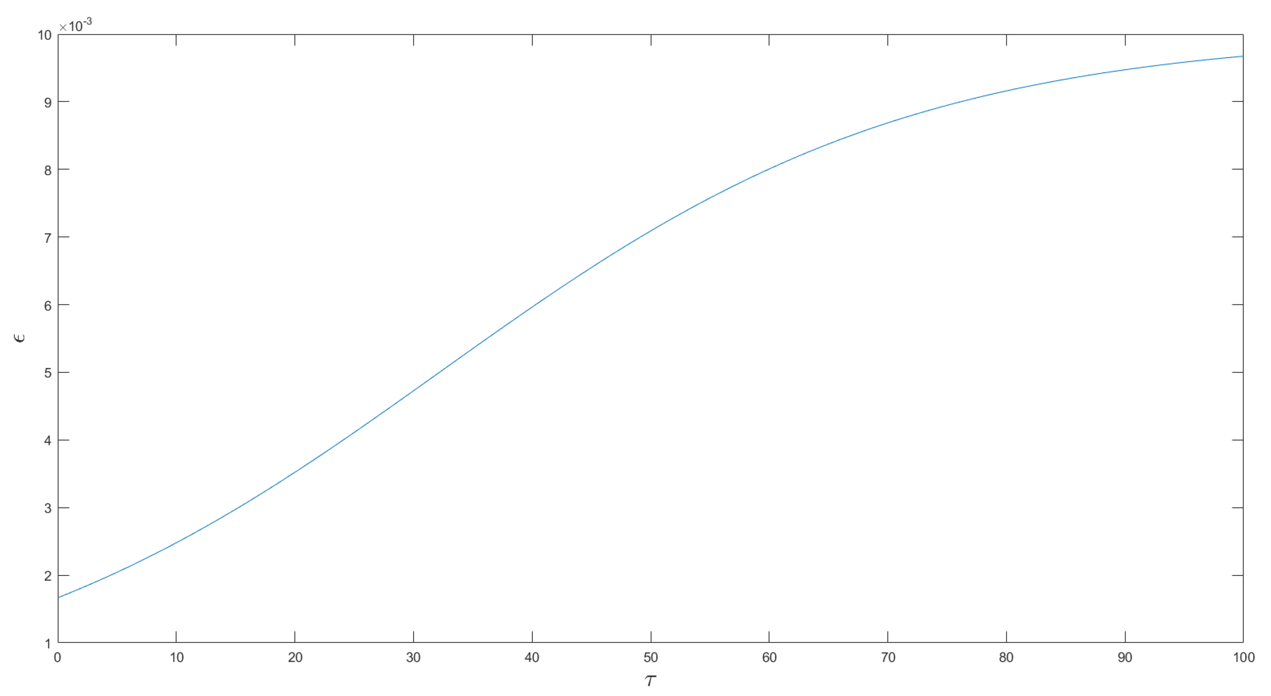
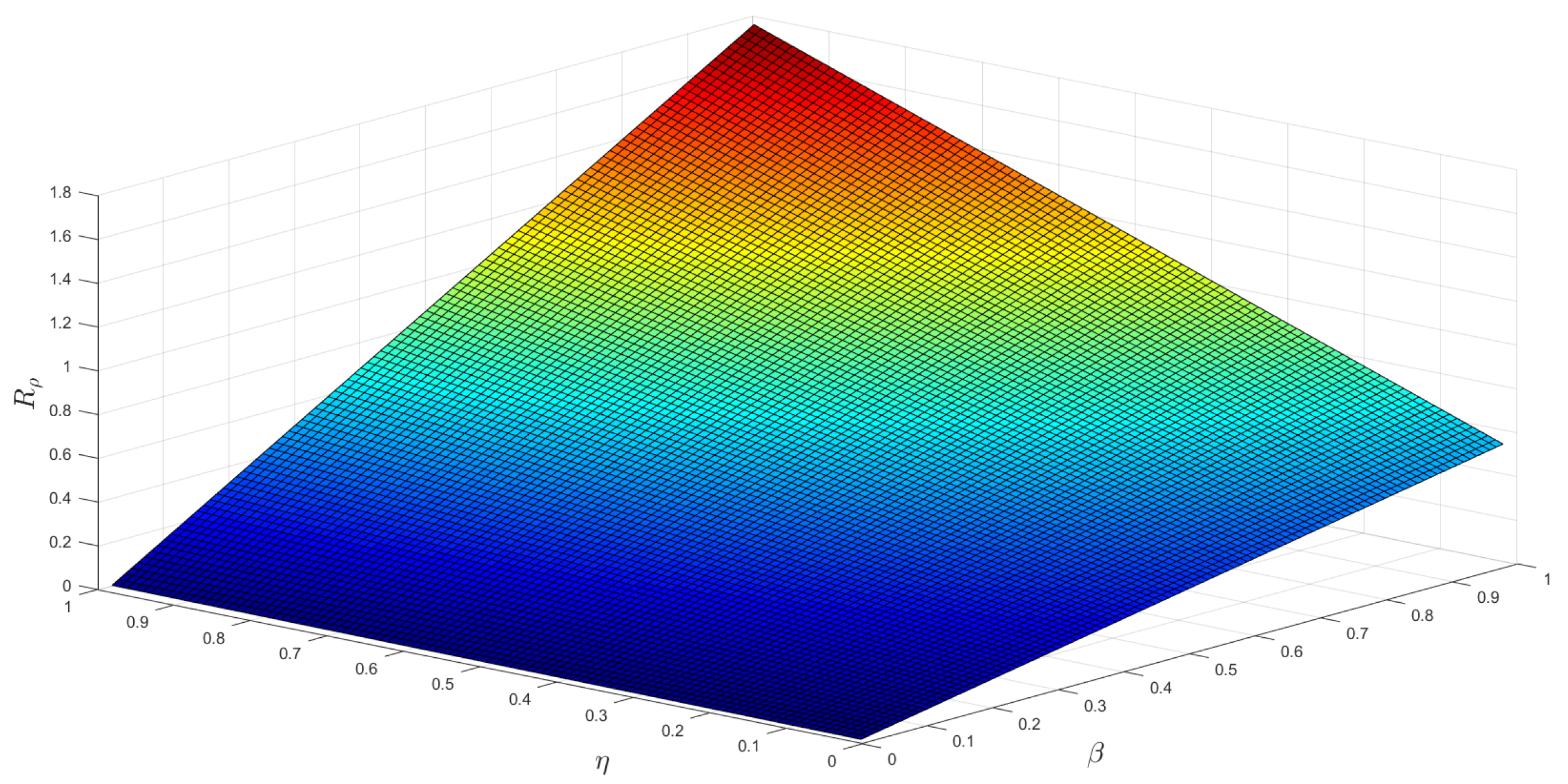
5. Numerical Simulations

In this section, we created a model using MATLAB and simulated the behavior of System (1). First, in order to investigate the relationship between the age-dependent conversion rate $\epsilon$ and age, based on [16,17,26,32], we assumed that the age-dependent conversion rate $\epsilon$ in the model took the following form: $\epsilon =\frac{0.01}{1+5e^{-0.05x}}$.

As depicted in Figure 2, the likelihood of the exposed individuals to become infected increases with age $\tau$.

To further investigate the relationship among the basic reproduction number $R_{\rho }$, the contact rate $\beta$ between infected individuals and individuals with susceptibility to the disease, and the effectiveness of imperfect vaccine $\eta$, we used $\mathsf{\Lambda }=1$, $\mu =0.3$, $\gamma =0.7$, $p=0.4$, ${\xi }_2=0.3$, $\kappa =0.8$, and

$$\epsilon \left(\tau \right)=\left\{\begin{array}{c}0,s\ge \tau \ge 0,\hfill \\ 0.3,\tau \ge s.\hfill \end{array}\right.$$

It can be seen from Figure 3 that the basic reproduction number $R_{\rho }$ is positively correlated with both $\eta$ and $\beta$. The $R_{\rho }$ increases as the probability $\eta$ and $\beta$ increase. Therefore, in order to reduce the infection rate of COVID-19, it is necessary to minimize the possibility of imperfect vaccination, i.e., to improve the effectiveness of the developed vaccine, and to reduce the contact rate of patients to individuals with susceptibility to the disease.

6. Conclusions

Based on the mechanism of COVID-19 infection in susceptible individuals, the present paper presented an SVEIR model considering imperfect vaccination and latent age. The age structure within a latent class was studied, where the latency was described by a variable associated with age, namely, the latent-disease conversion rate $\epsilon \left(\tau \right)$. The theorem of the next generation matrix was used to calculate the basic reproduction number $R_{\rho }$, which served as a crucial threshold for controlling the harm caused by COVID-19. When $R_{\rho }<1$, the disease-free equilibrium $\ddot{G}$ was globally asymptotically stable, which meant that the disease would eventually disappear. On the contrary, when $R_{\rho }>1$, the endemic equilibrium $\widehat{G}$ was globally asymptotically stable, suggesting that the disease would become endemic. Moreover, it was also necessary to analyze the asymptotic smoothness and uniform persistence of the semiflow generated by the system before proving the existence of the global attractor and applying the Lyapunov function method.

The results of this paper provide some suggestions for controlling COVID-19. It is necessary to minimize the likelihood of imperfect vaccination. This can be achieved not only by enhancing the effectiveness of the vaccine, but also by encouraging people to receive booster shots to maintain the long-term effectiveness of the vaccine. It is also essential to reduce the contact rate of patients with individuals who are susceptible to the disease, such as through a timely isolation of infected individuals.

References

1. Kermark, W.O.; Mckendrick, A.G. A contribution to the mathematical theory of epidemics. Proc. R. Soc. Lond. Ser. 1927, 115, 700–721. [Google Scholar]
2. Li, J.Y.; Yang, Y.L.; Zhou, Y.C. Global stability of an epidemic model with latent stage and vaccination. Nonlinear Anal. Real World Appl. 2011, 12, 2163–2173. [Google Scholar] [CrossRef]
3. Wang, J.L.; Huang, G.; Takeuchi, Y.; Liu, S. SVEIR epidemiological model with varying infectivity and distributed delays. Math. Biosci. Eng. 2011, 8, 875–888. [Google Scholar] [PubMed]
4. Upadhyay, R.K.; Kumari, S.; Misra, A.K. Modeling the virus dynamics in computer network with SVEIR model and nonlinear incident rate. J. Appl. Math. Comput. 2017, 54, 485–509. [Google Scholar] [CrossRef]
5. Zhang, Z.; Kundu, S.; Tripathi, J.P.; Bugalia, S. Stability and Hopf bifurcation analysis of an SVEIR epidemic model with vaccination and multiple time delays. Chaos Solitons Fractals 2020, 131, 109483. [Google Scholar] [CrossRef]
6. Castillo-Chavez, C.; Song, B. Dynamical models of tuberculosis and their applications. Math. Biosci. Eng. 2004, 1, 361–404. [Google Scholar] [CrossRef]
7. Zou, L.; Ruan, S.G.; Zhang, W.N. An age-structured model for the transmission dynamics of hepatitis B. Siam J. Appl. Math. 2010, 70, 3121–3139. [Google Scholar] [CrossRef] [Green Version]
8. Gumel, A.B.; McCluskey, C.C.; Watmough, J. An SVEIR Model for Assessing Potential Impact of an Imperfect Anti-Sars Vaccine. Math. Biosci. Eng. 2006, 3, 485–512. [Google Scholar] [PubMed]
9. Gumel, A.B.; McCluskey, C.C.; van den Driessche, P. Mathematical study of a staged progression HIV model with imperfect vaccine. Bull. Math. Biol. 2016, 68, 2105–2128. [Google Scholar] [CrossRef] [PubMed]
10. Röst, G. SEIR epidemiological model with varying infectivity and infinite delay. Math. Biosci. Eng. 2008, 5, 389–402. [Google Scholar]
11. Griffiths, J.; Lowrie, D.; Williams, J. An age-structured model for the AIDS epidemic. Eur. J. Oper. Res. 2000, 124, 1–14. [Google Scholar] [CrossRef]
12. Magal, P.; McCluskey, C.C.; Webb, G.F. Lyapunov functional and global asymptotic stability for an infection-age model. Appl. Anal. 2010, 89, 1109–1140. [Google Scholar] [CrossRef]
13. Inaba, H.; Sekine, H. A mathematical model for Chagas disease with infection-age-dependent infectivity. Math. Biosci. 2004, 190, 39–69. [Google Scholar] [CrossRef] [PubMed]
14. Ebenman, B. Niche differences between age classes and intraspecific competition in age-structured populations. J. Theor. Biol. 1987, 124, 25–33. [Google Scholar] [CrossRef]
15. Guo, Z.K.; Xiang, H.; Huo, H.F. Analysis of an age-structured tuberculosis model with treatment and relapse. J. Math. Biol. 2021, 82, 1–37. [Google Scholar] [CrossRef] [PubMed]
16. Xu, R. Global dynamics of an epidemiological model with age of infection and disease relapse. J. Biol. Dyn. 2018, 12, 118–145. [Google Scholar] [CrossRef] [Green Version]
17. Browne, C.J.; Plyugin, S.S. Global analysis of age-structured within-host virus model. Discret. Contin. Dyn. Syst. Ser. 2013, 18, 1999–2017. [Google Scholar] [CrossRef]
18. Dai, W.H.; Zhang, H.L. Dynamical analysis for an age-structured model of eating disorders. J. Appl. Math. Comput. 2023, 69, 1887–1901. [Google Scholar] [CrossRef]
19. Kenne, C.; Mophou, G.; Dorville, R.; Zongo, P. A model for brucellosis disease incorporating age of infection and waning immunity. Mathematics 2022, 10, 670. [Google Scholar] [CrossRef]
20. Li, H.; Wang, J. Global dynamics of an SEIR model with the age of infection and vaccination. Mathematics 2021, 9, 2195. [Google Scholar] [CrossRef]
21. Wang, Y.P.; Hu, L.; Nie, L.F. Dynamics of a hybrid HIV/AIDS model with age-structured, self-protection and media coverage. Mathematics 2023, 11, 82. [Google Scholar] [CrossRef]
22. He, Z.R.; Zhou, N. Controll ability and stabilization of a nonlinear hierarchical age-structured competing system. Electron. J. Differ. Equ. 2020, 2020, 1–16. [Google Scholar]
23. Liu, L.L.; Liu, X.N. Global stability of an age-structured SVEIR epidemic model with waning immunity, latency and relapse. Int. J. Biomath. 2017, 10, 1750038. [Google Scholar] [CrossRef]
24. Huo, H.F.; Yang, P.; Xiang, H. Dynamics for an SIRS epidemic model with infection age and relapse on a scale-free network. J. Frankl.-Inst.-Eng. Appl. Math. 2019, 356, 7411–7443. [Google Scholar] [CrossRef]
25. Khan, A.; Zaman, G. Optimal control strategy of SEIR endemic model with continuous age-structure in the exposed and infectious classes. Optim. Control. Appl. Methods 2018, 39, 1716–1727. [Google Scholar] [CrossRef]
26. Diekmann, O.; Heesterbeek, J.A.P.; Metz, J.A. On the definition and the computation of the basic reproduction ratio in models for infectious diseases in heterogeneous populations. J. Math. Biol. 1990, 28, 365–382. [Google Scholar] [CrossRef] [Green Version]
27. Hale, J.K. Functional Differential Equations. In Analytic Theory of Differential Equations, Proceedings of the Conference at Western Michigan University, Kalamazoo, MI, USA, 30 April–2 May 1970; Springer: Berlin/Heidelberg, Germany, 1970; pp. 9–22. [Google Scholar]
28. Hale, J.K.; Waltman, P. Persistence in infinite-dimensional systems. Siam J. Math. Anal. 1989, 20, 388–395. [Google Scholar] [CrossRef]
29. Adams, R.A.; Fournier, J.J. Sobolev Space; Academic Press: New York, NY, USA, 2003; pp. 38–40. [Google Scholar]
30. McCluskey, C.C. Global stability for an SEI epidemiological model with continuous age-structure in the exposed and infectious classes. Math. Biosci. Eng. 2005, 9, 819–841. [Google Scholar]
31. Magal, P. Compact attractors for time-periodic age-structured population models. Electron. J. Differ. Equ. 2001, 2001, 1–35. [Google Scholar]
32. Magal, P. Global attractors and steady states for uniformly persistent dynamical systems. Siam J. Math. Anal. 2005, 37, 251–275. [Google Scholar] [CrossRef] [Green Version]
Figure 1. Compartment transfer diagram of the model.
Mathematics 11 03526 g001
Figure 2. Age–dependent conversion rate during latency.
Mathematics 11 03526 g002
Figure 3. Relationships among R ρ , β , and η at fixed parameters.
Mathematics 11 03526 g003
Disclaimer/Publisher’s Note: The statements, opinions and data contained in all publications are solely those of the individual author(s) and contributor(s) and not of MDPI and/or the editor(s). MDPI and/or the editor(s) disclaim responsibility for any injury to people or property resulting from any ideas, methods, instructions or products referred to in the content.