On the Dynamical Behavior of Solitary Waves for Coupled Stochastic Korteweg–De Vries Equations

Abstract

In this paper, we take into account the coupled stochastic Korteweg–De Vries (CSKdV) equations in the Itô sense. Using the mapping method, new trigonometric, rational, hyperbolic, and elliptic stochastic solutions are obtained. These obtained solutions can be applied to the analysis of a wide variety of crucial physical phenomena because the coupled KdV equations have important applications in various fields of physics and engineering. Also, it is used in the design of optical fiber communication systems, which transmit information using soliton-like waves. The dynamic performance of the various obtained solutions are depicted using 3D and 2D curves in order to interpret the effects of multiplicative noise. We conclude that multiplicative noise influences the behavior of the solutions of CSKdV equations and stabilizes them.

1. Introduction

Stochastic partial differential equations (SPDEs) are mathematical models designed to describe the evolution of systems which exhibit randomness. These equations have been developed for a variety of applications across fields in physics, engineering, and finance, among others [1,2]. Unlike deterministic models, SPDEs take into account the presence of random variables, which have a significant impact on the system’s behavior. Therefore, they provide a more comprehensive and realistic representation of the system’s dynamics. This essay will provide an overview of SPDEs, discuss their applications, and highlight some of the challenges associated with their analysis.

The study of SPDEs has gained significant attention due to their wide application across various fields, such as turbulence, climate modeling, financial engineering, materials science, biology, and neuroscience. For instance, SPDEs have been used to model the behavior of turbulent fluids, which are characterized by their chaotic and unpredictable nature. In climate modeling, scientists use SPDEs to account for the impact of uncertain factors, such as solar radiation and greenhouse gas emissions, in the prediction of climate patterns. Similarly, financial engineers use SPDEs to model the fluctuations in stock prices and interest rates, which are subject to unexpected shocks and volatility.

One of the primary challenges of SPDEs is the need to derive exact solutions. Recently, many authors obtained the exact solutions for some SPDEs, such as the Maccari system [3], mKdV equation [4], Davey–Stewartson equation [5], Jimbo–Miwa equation [6], $(4+1)$-dimensional Fokas equation [7], etc.

In this paper, we consider the following coupled stochastic Korteweg–De Vries (CSKdV) equations:

$$\begin{array}{c}{\Phi }_t={\Phi }_{xxx}+6\Phi {\Phi }_x+2\Psi {\Psi }_x+\sigma \Phi {\mathcal{W}}_t,\hfill \\ \\ {\Psi }_t=-{\Psi }_{xxx}-3\Phi {\Psi }_x+\sigma \Psi {\mathcal{W}}_t,\hfill \end{array}$$

(1)

where $\Phi =\Phi (x,t)$ and $\Psi =\Psi (x,t)$ are the wave amplitudes. $\sigma$ is a positive constant, $\mathcal{W}(t)$ is the standard Wiener process (SWP) and ${\mathcal{W}}_t=\frac{\partial \mathcal{W}}{\partial t}$. When Wu et al. [8] investigated a $4\times 4$ matrix spectral problem with three potentials, they obtained Equation (1) with $\sigma =0$. If we put $\Psi =0$, then we obtain the well-known KdV equation. The KdV equation explains the propagation of a single soliton wave in an infinitely long and uniform water channel. However, in a real medium, the waves interact with each other. The coupled KdV equations address this interaction by considering a system of two or more waves propagating in the same medium.

Coupled KdV equations have significant uses in numerous disciplines of physics and engineering. For example, they have been used to study the formation and propagation of ocean waves and atmospheric waves. In addition, they have also been used in the study of Bose–Einstein condensates, which are ultra-cold gases of atoms that behave like waves. Coupled KdV equations have also been used in the design of optical fiber communication systems, which transmit information using soliton-like waves. Due to the importance of coupled KdV equations, many authors have obtained the exact solutions for this equation by using different methods, including the generalized tanh function method [9], F-expansion method [10], improved homogeneous balance method [11], and algebra method [12]. The CSKdV Equation (1) has not been studied until now.

The novelty of this work is the acquisition of the exact stochastic solutions of the CSKdV Equation (1). We employ a mapping method (M-method) to arrive at these solutions. This method is more general than many others, such as the tanh–coth method, the sine–cosine method, and the elliptic function method, because the solutions we derive from this method can take various forms, including trigonometric, rational, hyperbolic, and elliptic functions. Therefore, we generalize some of the previous results stated in [9]. Using the stochastic term in Equation (1), the solutions would be extremely useful to physicists in defining a broad range of critical physical phenomena. To address the influence of the stochastic term on the obtained solution of the CSKdV Equation (1), we give a large number of figures by using MATLAB.

The outline of this study is as follows: The wave equation of CSKdV Equation (1) is obtained in Section 2, while the mapping method is explained in Section 3. In Section 4, we obtain the exact solutions of the CSKdV Equation (1). In Section 5, we are able to examine how the stochastic term influences the solutions that are produced for the CSKdV Equation (1). Finally, the conclusions of this study are given.

2. Traveling Wave Equation for Coupled SKdV Equations

To attain the wave equation for CSKdV Equation (1), we utilize

$$\Phi (x,t)=\phi (\zeta )e^{\sigma \mathcal{W}-\frac{1}{2}{\sigma }^{2}t}\mathrm{and}\Psi (x,t)=\psi (\zeta )e^{\sigma \mathcal{W}-\frac{1}{2}{\sigma }^{2}t},\zeta =kx+\lambda t,$$

(2)

where $\phi$ and $\psi$ are real functions and deterministic, and k and $\lambda$ are non-zero constants. We observe that

$$\begin{array}{ccc}{\Phi }_t\hfill & =& [\lambda {\phi }^{\prime }+\sigma \phi {\mathcal{W}}_t-\frac{1}{2}{\sigma }^2\phi +\frac{1}{2}{\sigma }^2\phi ]e^{\sigma \mathcal{W}-\frac{1}{2}{\sigma }^{2}t}\hfill \\ & =& [\lambda {\phi }^{\prime }+\sigma \phi {\mathcal{W}}_t]e^{\sigma \mathcal{W}-\frac{1}{2}{\sigma }^{2}t},\hfill \\ {\Phi }_x\hfill & =& k{\phi }^{\prime }{e}^{\sigma \mathcal{W}-\frac{1}{2}{\sigma }^{2}t},{\Phi }_{xxx}=k^3{\phi }^{‴}{e}^{\sigma \mathcal{W}-\frac{1}{2}{\sigma }^{2}t},\hfill \end{array}$$

(3)

where $\frac{1}{2}{\sigma }^2\phi$ is the Itô correction term. Similarly,

$${\Psi }_t=[\lambda {\psi }^{\prime }+\sigma \psi {\mathcal{W}}_t]e^{\sigma \mathcal{W}-\frac{1}{2}{\sigma }^{2}t},{\Psi }_x=k{\psi }^{\prime }{e}^{\sigma \mathcal{W}-\frac{1}{2}{\sigma }^{2}t},{\Psi }_{xxx}=k^3{\psi }^{‴}{e}^{\sigma \mathcal{W}-\frac{1}{2}{\sigma }^{2}t}.$$

(4)

Substituting Equations (3) and (4) into Equation (1), we obtain

$$\begin{array}{c}{k}^3{\phi }^{‴}+6k\phi {\phi }^{\prime }{e}^{\sigma \mathcal{W}-\frac{1}{2}{\sigma }^{2}t}+2k\psi {\psi }^{\prime }{e}^{\sigma \mathcal{W}-\frac{1}{2}{\sigma }^{2}t}-\lambda {\phi }^{\prime }=0,\hfill \\ \\ k^3{\psi }^{‴}+3k\phi {\psi }^{\prime }{e}^{\sigma \mathcal{W}-\frac{1}{2}{\sigma }^{2}t}+\lambda {\psi }^{\prime }=0.\hfill \end{array}$$

(5)

Now, we take the expectation on both sides of Equation (5) to obtain

$$\begin{array}{c}{k}^3{\phi }^{‴}+6k\phi {\phi }^{\prime }{e}^{-\frac{1}{2}{\sigma }^{2}t}\mathbb{E}(e^{\sigma \mathcal{W}})-\lambda {\phi }^{\prime }+2k\psi {\psi }^{\prime }{e}^{-\frac{1}{2}{\sigma }^{2}t}\mathbb{E}(e^{\sigma \mathcal{W}})=0,\hfill \\ \\ k^3{\psi }^{‴}+\lambda {\psi }^{\prime }+3k\phi {\psi }^{\prime }{e}^{-\frac{1}{2}{\sigma }^{2}t}\mathbb{E}(e^{\sigma \mathcal{W}})=0.\hfill \end{array}$$

(6)

Since $\mathcal{W}(t)$ is a normal process, then $\mathbb{E}(e^{\sigma \mathcal{W}})=e^{\frac{1}{2}{\sigma }^{2}t}$ for any real number $\sigma$. Hence, Equation (6) takes the form

$$\begin{array}{c}{k}^3{\phi }^{‴}+6k\phi {\phi }^{\prime }-\lambda {\phi }^{\prime }+2k\psi {\psi }^{\prime }=0,\hfill \\ \\ k^3{\psi }^{‴}+\lambda {\psi }^{\prime }+3k\phi {\psi }^{\prime }=0.\hfill \end{array}$$

(7)

Integrating the first equation from Equation (7) once, we obtain

$$\begin{array}{c}{k}^3{\phi }^{″}+3k{\phi }^2-\lambda \phi +k{\psi }^2=0,\hfill \\ \\ k^3{\psi }^{‴}+\lambda {\psi }^{\prime }+3k\phi {\psi }^{\prime }=0.\hfill \end{array}$$

(8)

3. The Clarification of M-Method

Here, the mapping method described in [13] is applied. Let the solutions of Equation (8) take the form

$$\begin{array}{c}\phi (\zeta )=\sum _{i=0}^{N_1}{\mathsf{\ell }}_i{u}^i(\zeta ),\hfill \\ \\ \psi (\zeta )=\sum _{i=0}^{N_2}{\varpi }_i{u}^i(\zeta ),\hfill \end{array}$$

(9)

where ${\mathsf{\ell }}_i$ and ${\varpi }_i$ are undetermined constants to be calculated, and u solves

$$u^{\prime }=\sqrt{q{u}^4+p{u}^2+r},$$

(10)

where the parameters $q,p$, and r are all real numbers. For $r,q$ and $p,$Equation (10) has several solutions as follows:

$sn(\zeta )=sn(\zeta ,m),$ $dn(\zeta )=dn(\zeta ,m),cn(\zeta )=cn(\zeta ,m),$ are the Jacobi elliptic functions (JEFs) for $0<m<1.$

The following trigonometric functions are generated from JEFs when $m\to 0:$

$$\begin{array}{ccc}sn(\zeta )\hfill & \to & sin(\zeta ),cs(\zeta )\to cot(\zeta ),\hfill \\ cn(\zeta )\hfill & \to & cos(\zeta ),ds\to csc(\zeta ),dn(\zeta )\to 1.\hfill \end{array}$$

Furthermore, the following hyperbolic functions are generated from JEFs when $m\to 1$:

$$\begin{array}{ccc}sn(\zeta )\hfill & \to & tanh(\zeta ),cn(\zeta )\to \mathrm{sech}(\zeta ),dn(\zeta )\to \mathrm{sech}(\zeta ),\hfill \\ ds\hfill & \to & \mathrm{csch}(\zeta ),cs(\zeta )\to \mathrm{csch}(\zeta ).\hfill \end{array}$$

4. Exact Solutions of the CSKdV Equations

First, let us balance ${\phi }^{″}$ with ${\phi }^2$ and ${\psi }^{‴}$with $\phi {\psi }^{\prime }$ in Equation (8) to determine the parameter $N_1$ and $N_2$ as

$$N_1=2\mathrm{and}{N}_2=1.$$

With $N_1=2$and $N_2=1$, Equation (9) takes the form

$$\begin{array}{c}\phi (\zeta )={\mathsf{\ell }}_0+{\mathsf{\ell }}_{1}u(\zeta )+{\mathsf{\ell }}_2{u}^2(\zeta ),\hfill \\ \\ \psi (\zeta )={\varpi }_0+{\varpi }_{1}u(\zeta ).\hfill \end{array}$$

(11)

Putting Equation (11) into Equation (8), we obtain

$$\begin{array}{ccc}& & (3k{\mathsf{\ell }}_2^2+6k^3{\mathsf{\ell }}_2)u^4+(6k{\mathsf{\ell }}_0{\mathsf{\ell }}_2+k{\varpi }_1-{\mathsf{\ell }}_2\lambda )u^2+(2k{\varpi }_0{\varpi }_1)u\hfill \\ & & +(2r{\mathsf{\ell }}_2{k}^2+k{\varpi }_0^2+3k{\mathsf{\ell }}_0^2-\lambda {\mathsf{\ell }}_0)=0,\hfill \end{array}$$

and

$$(\lambda {\varpi }_1+3k{\mathsf{\ell }}_0{\varpi }_1+{\varpi }_{1}p{k}^3)u^{\prime }+(3k{\varpi }_1)u{u}^{\prime }+(3k{\mathsf{\ell }}_2{\varpi }_1+6k^{3}q{\varpi }_1)u^2{u}^{\prime }=0.$$

For $j=3,2,1,0,$ we balance each coefficient of $u^j$ and $u^j{u}^{\prime }$ with zero to have

$$3k{\mathsf{\ell }}_2^2+6k^3{\mathsf{\ell }}_2=0,$$

$$6k{\mathsf{\ell }}_0{\mathsf{\ell }}_2+k{\varpi }_1-{\mathsf{\ell }}_2\lambda =0,$$

$$2k{\varpi }_0{\varpi }_1=0,$$

$$2r{\mathsf{\ell }}_2{k}^2+k{\varpi }_0^2+3k{\mathsf{\ell }}_0^2-\lambda {\mathsf{\ell }}_0=0,$$

and

$$3k{\mathsf{\ell }}_2{\varpi }_1+6k^{3}q{\varpi }_1=0,$$

$$3k{\varpi }_1=0,$$

$$\lambda {\varpi }_1+3k{\mathsf{\ell }}_0{\varpi }_1+{\varpi }_{1}p{k}^3=0.$$

We obtain two different families when we solve these equations for $96rq+p^2>0$:

Family-1:

$$\begin{array}{c}{\mathsf{\ell }}_0=\frac{-p{k}^2}{12}+\frac{p{k}^2}{12}\sqrt{96rq+p^2},{\mathsf{\ell }}_1=0,{\mathsf{\ell }}_2=-2q{k}^2,{\varpi }_0=0,\hfill \\ \\ {\varpi }_1=\frac{pq{k}^4}{12}+\frac{3k^4}{2}\sqrt{96rq+p^2},\lambda =\frac{-3p{k}^3}{4}-\frac{k^3}{4}\sqrt{96rq+p^2}.\hfill \end{array}$$

(12)

Family-2:

$$\begin{array}{c}{\mathsf{\ell }}_0=\frac{-p{k}^2}{12}-\frac{p{k}^2}{12}\sqrt{96rq+p^2},{\mathsf{\ell }}_1=0,{\mathsf{\ell }}_2=-2q{k}^2,{\varpi }_0=0,\hfill \\ \\ {\varpi }_1=\frac{pq{k}^4}{12}-\frac{3k^4}{2}\sqrt{96rq+p^2},\lambda =\frac{-3p{k}^3}{4}+\frac{k^3}{4}\sqrt{96rq+p^2}.\hfill \end{array}$$

(13)

Family-1: By utilizing Equations (2), (11) and (12), the solutions of Equation (1) are

$$\Phi (x,t)=[\frac{-p{k}^2}{12}+\frac{p{k}^2}{12}\sqrt{96rq+p^2}-2q{k}^2{u}^2(\zeta )]e^{\sigma \mathcal{W}-\frac{1}{2}{\sigma }^{2}t},$$

(14)

and

$$\Psi (x,t)=[\frac{pq{k}^4}{12}+\frac{3k^4}{2}\sqrt{96rq+p^2}]u(\zeta )e^{\sigma \mathcal{W}-\frac{1}{2}{\sigma }^{2}t},$$

(15)

where $\zeta =kx+(\frac{-3p{k}^3}{4}-\frac{k^3}{4}\sqrt{96rq+p^2})t$. There are many cases depending on $r,q$ and p as shown in Table 1 such that $96rq+p^2>0:$

Table 1. Solutions for Equation (10) for different values of $r,q$ and p.

Case	q	p	r	$\mathit{u}(\mathit{\zeta })$
1	$m^2$	$-(1+m^2)$	1	$sn(\zeta )$
2	1	$2-m^2$	$(1-m^2)$	$cs(\zeta )$
3	$\frac{m^2}{4}$	$\frac{(m^2-2)}{2}$	$\frac{1}{4}$	$\frac{sn(\zeta )}{1+dn(\zeta )}$
4	$\frac{{(1-m^2)}^2}{4}$	$\frac{{(1-m^2)}^2}{2}$	$\frac{1}{4}$	$\frac{sn(\zeta )}{dn+cn(\zeta )}$
5	$\frac{1-m^2}{4}$	$\frac{(1-m^2)}{2}$	$\frac{(1-m^2)}{4}$	$\frac{cn(\zeta )}{1+sn(\zeta )}$
6	$-1$	$2-m^2$	$(m^2-1)$	$dn(\zeta )$
7	$-m^2$	$2m^2-1$	$(1-m^2)$	$cn(\zeta )$
8	$\frac{m^2-1}{4}$	$\frac{(m^2+1)}{2}$	$\frac{(m^2-1)}{4}$	$\frac{dn(\zeta )}{1+sn(\zeta )}$
9	$\frac{-1}{4}$	$\frac{(m^2+1)}{2}$	$\frac{-{(1-m^2)}^2}{4}$	m$cn($$\zeta$$)\pm dn($$\zeta$)

Case 1-1: If $q=m^2,p=-(1+m^2)$ and$r=1,$ then $u(\zeta )=sn(\zeta ).$ Thus, using Equations (14) and (15), the solutions of the CSKdV Equation (1) are

$$\begin{array}{ccc}\Phi (x,t)\hfill & =& [\frac{(1+m^2)k^2}{12}-\frac{(1+m^2)k^2}{12}\sqrt{96m^2+{(1+m^2)}^2}\hfill \\ & & -2m^2{k}^{2}s{n}^2(\zeta )]e^{\sigma \mathcal{W}-\frac{1}{2}{\sigma }^{2}t},\hfill \end{array}$$

(16)

$$\Psi (x,t)=[\frac{-m^2(1+m^2)k^4}{12}+\frac{3k^4}{2}\sqrt{96m^2+{(1+m^2)}^2}]sn(\zeta )e^{\sigma \mathcal{W}-\frac{1}{2}{\sigma }^{2}t}.$$

(17)

If $m\to 1,$ Equations (16) and (17) become

$$\Phi (x,t)=[\frac{-3k^2}{2}-2k^2{tanh}^2(kx-k^{3}t)]e^{\sigma \mathcal{W}-\frac{1}{2}{\sigma }^{2}t},$$

(18)

$$\Psi (x,t)=\frac{89k^4}{6}tanh(kx-k^{3}t)e^{\sigma \mathcal{W}-\frac{1}{2}{\sigma }^{2}t}.$$

(19)

Case 1-2: If $q=1,p=2-m^2$ and$r=(1-m^2),$ then $u(\zeta )=cs(\zeta ).$ Thus, using Equations (14) and (15), the solutions of the CSKdV Equation (1) are

$$\begin{array}{ccc}\Phi (x,t)\hfill & =& [\frac{-(2-m^2)k^2}{12}+\frac{(2-m^2)k^2}{12}\sqrt{96(1-m^2)+{(2-m^2)}^2}\hfill \\ & & -2k^{2}c{s}^2(\zeta )]e^{\sigma \mathcal{W}-\frac{1}{2}{\sigma }^{2}t},\hfill \end{array}$$

(20)

$$\Psi (x,t)=[\frac{(2-m^2)k^4}{12}+\frac{3k^4}{2}\sqrt{96(1-m^2)+{(2-m^2)}^2}]cs(\zeta )e^{\sigma \mathcal{W}-\frac{1}{2}{\sigma }^{2}t}.$$

(21)

If $m\to 1,$ Equations (20) and (21) become

$$\Phi (x,t)=-2k^2{\mathrm{csch}}^2(kx-k^{3}t)e^{\sigma \mathcal{W}-\frac{1}{2}{\sigma }^{2}t},$$

(22)

$$\Psi (x,t)=\frac{19k^4}{12}\mathrm{csch}(kx-k^{3}t)e^{\sigma \mathcal{W}-\frac{1}{2}{\sigma }^{2}t}.$$

(23)

If $m\to 0,$ Equations (20) and (21) become

$$\Phi (x,t)=[\frac{3k^2}{2}-2k^2{cot}^2(kx-4k^{3}t)]e^{\sigma \mathcal{W}-\frac{1}{2}{\sigma }^{2}t},$$

(24)

$$\Psi (x,t)=\frac{91k^4}{6}cot(kx-4k^{3}t)e^{\sigma \mathcal{W}-\frac{1}{2}{\sigma }^{2}t}.$$

(25)

Case 1-3: If $q=\frac{m^2}{4},p=\frac{(m^2-2)}{2}$ and$r=\frac{1}{4},$ then $u(\zeta )=\frac{sn(\zeta )}{1+dn(\zeta )}.$ Thus, using Equations (14) and (15), the solutions of the CSKdV Equation (1) are

$$\begin{array}{ccc}\Phi (x,t)\hfill & =& [\frac{-(m^2-2)k^2}{24}+\frac{(m^2-2)k^2}{24}\sqrt{6m^2+\frac{{(m^2-2)}^2}{4}}\hfill \\ & & -\frac{m^2}{2}{k}^2{(\frac{sn(\zeta )}{1+dn(\zeta )})}^2]e^{\sigma \mathcal{W}-\frac{1}{2}{\sigma }^{2}t},\hfill \end{array}$$

(26)

$$\Psi (x,t)=[\frac{m^2(m^2-2)k^4}{96}+\frac{3k^4}{2}\sqrt{6m^2+\frac{{(m^2-2)}^2}{4}}](\frac{sn(\zeta )}{1+dn(\zeta )})e^{\sigma \mathcal{W}-\frac{1}{2}{\sigma }^{2}t}.$$

(27)

If $m\to 1,$ then Equations (26) and (27) tend to

$$\Phi (x,t)=[\frac{-k^2}{16}-\frac{1}{2}{k}^2{(\frac{tanh(kx-\frac{11}{24}{k}^{3}t)}{1+\mathrm{sech}(kx-\frac{11}{24}{k}^{3}t)})}^2]e^{\sigma \mathcal{W}-\frac{1}{2}{\sigma }^{2}t},$$

(28)

$$\Psi (x,t)=\frac{359k^4}{96}(\frac{tanh(kx-\frac{11}{24}{k}^{3}t)}{1+\mathrm{sech}(kx-\frac{11}{24}{k}^{3}t)})e^{\sigma \mathcal{W}-\frac{1}{2}{\sigma }^{2}t}.$$

(29)

Case 1-4: If $p=\frac{{(1-m^2)}^2}{4},q=\frac{{(1-m^2)}^2}{2}$ and$r=\frac{1}{4},$ then $u(\zeta )=\frac{sn(\zeta )}{dn(\zeta )+cn(\zeta )}.$ Thus, using Equations (14) and (15), the solutions of the CSKdV Equation (1) are

$$\begin{array}{ccc}\Phi (x,t)\hfill & =& k^2{(1-m^2)}^2[\frac{-1}{48}+\frac{1}{48}\sqrt{12{(1-m^2)}^2+\frac{{(1-m^2)}^4}{16}}\hfill \\ & & -{(\frac{sn(\zeta )}{dn(\zeta )+cn(\zeta )})}^2]e^{\sigma \mathcal{W}-\frac{1}{2}{\sigma }^{2}t},\hfill \end{array}$$

(30)

$$\begin{array}{ccc}\Psi (x,t)\hfill & =& e^{\sigma \mathcal{W}-\frac{1}{2}{\sigma }^{2}t}[\frac{{(1-m^2)}^2{k}^4}{96}+\hfill \\ & & +\frac{3k^4}{2}\sqrt{12{(1-m^2)}^2+\frac{{(1-m^2)}^4}{16}}](\frac{sn(\zeta )}{dn(\zeta )+cn(\zeta )}).\hfill \end{array}$$

(31)

When $m\to 0$, Equations (30) and (31) tend to

$$\Phi (x,t)=[\frac{-k^2}{48}+\frac{k^2}{192}\sqrt{193}-k^2{(\frac{sin(kx-\frac{k^3}{16}(3+\sqrt{193})t)}{1+cos(kx-\frac{k^3}{16}(3+\sqrt{193})t)})}^2]e^{\sigma \mathcal{W}-\frac{1}{2}{\sigma }^{2}t},$$

(32)

$$\Psi (x,t)=[\frac{k^4}{96}+\frac{3k^4}{8}\sqrt{193}](\frac{sin(kx-\frac{k^3}{16}(3+\sqrt{193})t)}{1+cos(kx-\frac{k^3}{16}(3+\sqrt{193})t)})e^{\sigma \mathcal{W}-\frac{1}{2}{\sigma }^{2}t}.$$

(33)

Case 1-5: If $q=\frac{1-m^2}{4},p=\frac{(1-m^2)}{2}$ and$r=\frac{1-m^2}{4},$ then $u(\zeta )=\frac{cn(\zeta )}{1+sn(\zeta )}.$Thus, using Equations (14) and (15), the solutions of the CSKdV Equation (1) are

$$\begin{array}{ccc}\Phi (x,t)\hfill & =& \frac{k^2(1-m^2)}{4}[\frac{-1}{6}+\frac{1}{6}\sqrt{6{(1-m^2)}^2+\frac{{(1-m^2)}^2}{4}}\hfill \\ & & -2{(\frac{cn(\zeta )}{1+sn(\zeta )})}^2]e^{\sigma \mathcal{W}-\frac{1}{2}{\sigma }^{2}t},\hfill \end{array}$$

(34)

$$\Psi (x,t)=[\frac{{(1-m^2)}^2{k}^4}{96}+\frac{3k^4}{2}\sqrt{6{(1-m^2)}^2+\frac{{(1-m^2)}^2}{4}}](\frac{cn(\zeta )}{1+sn(\zeta )})e^{\sigma \mathcal{W}-\frac{1}{2}{\sigma }^{2}t}.$$

(35)

When $m\to 0,$ Equations (34) and (35) tend to

$$\Phi (x,t)=[\frac{k^2}{4}-2q{k}^2{(\frac{cos(kx-\frac{1}{2}{k}^{3}t)}{1+sin(kx-\frac{1}{2}{k}^{3}t)})}^2]e^{\sigma \mathcal{W}-\frac{1}{2}{\sigma }^{2}t},$$

(36)

$$\Psi (x,t)=\frac{361k^4}{96}(\frac{cos(kx-\frac{1}{2}{k}^{3}t)}{1+sin(kx-\frac{1}{2}{k}^{3}t)})e^{\sigma \mathcal{W}-\frac{1}{2}{\sigma }^{2}t}.$$

(37)

Case 1-6: If $q=-1,p=(2-m^2)$ and$r=m^2-1,$ then $u(\zeta )=dn(\zeta ).$Thus, using Equations (14) and (15), the solutions of the CSKdV Equation (1) are

$$\begin{array}{ccc}\Phi (x,t)\hfill & =& [\frac{-(2-m^2)k^2}{12}+\frac{(2-m^2)k^2}{12}\sqrt{96(1-m^2)+{(2-m^2)}^2}\hfill \\ & & +2k^2{(dn(\zeta ))}^2]e^{\sigma \mathcal{W}-\frac{1}{2}{\sigma }^{2}t},\hfill \end{array}$$

(38)

$$\Psi (x,t)=[\frac{(m^2-2)k^4}{12}+\frac{3k^4}{2}\sqrt{96(1-m^2)+{(2-m^2)}^2}]dn(\zeta )e^{\sigma \mathcal{W}-\frac{1}{2}{\sigma }^{2}t}.$$

(39)

If $m\to 1,$ then Equations (38) and (39) tend to

$$\Phi (x,t)=[2k^2{\mathrm{sech}}^2(kx-k^{3}t)]e^{\sigma \mathcal{W}-\frac{1}{2}{\sigma }^{2}t},$$

(40)

$$\Psi (x,t)=\frac{17k^4}{12}\mathrm{sech}(kx-k^{3}t)e^{\sigma \mathcal{W}-\frac{1}{2}{\sigma }^{2}t}.$$

(41)

When $m\to 0,$ Equations (38) and (39) tend to

$$\Phi (x,t)=\frac{7k^2}{2}{e}^{\sigma \mathcal{W}-\frac{1}{2}{\sigma }^{2}t},$$

(42)

$$\Psi (x,t)=\frac{89k^4}{6}{e}^{\sigma \mathcal{W}-\frac{1}{2}{\sigma }^{2}t},$$

(43)

Case 1-7: If $q=-m^2,p=(2m^2-1)$ and$r=1-m^2,$ then $u(\zeta )=cn(\zeta ).$Thus, using Equations (14) and (15), the solutions of the CSKdV Equation (1) are

$$\begin{array}{ccc}\Phi (x,t)\hfill & =& e^{\sigma \mathcal{W}-\frac{1}{2}{\sigma }^{2}t}[\frac{-(2m^2-1)k^2}{12}+\hfill \\ & & +\frac{(2m^2-1)k^2}{12}\sqrt{100m^4-100m^2+1}+2m^2{k}^{2}c{n}^2(\zeta )],\hfill \end{array}$$

(44)

and

$$\Psi (x,t)=[\frac{(m^2-2m^4)k^4}{12}+\frac{3k^4}{2}\sqrt{100m^4-100m^2+1}]cn(\zeta )e^{\sigma \mathcal{W}-\frac{1}{2}{\sigma }^{2}t}.$$

(45)

If $m\to 1,$ then Equations (44) and (45) tend to

$$\Phi (x,t)=2k^2{\mathrm{sech}}^2(kx-k^{3}t)e^{\sigma \mathcal{W}-\frac{1}{2}{\sigma }^{2}t},$$

(46)

$$\Psi (x,t)=\frac{17k^4}{12}\mathrm{sech}(kx-k^{3}t)e^{\sigma \mathcal{W}-\frac{1}{2}{\sigma }^{2}t}.$$

(47)

Case 1-8: If $q=\frac{m^2-1}{4},p=\frac{m^2+1}{4}$ and$r=\frac{m^2-1}{4},$ then $u(\zeta )=\frac{dn(\zeta )}{1+sn(\zeta )}.$Thus, using Equations (14) and (15), the solutions of the CSKdV Equations (1) are

$$\begin{array}{ccc}\Phi (x,t)\hfill & =& [\frac{-(m^2+1)k^2}{48}+\frac{(m^2+1)k^2}{48}\sqrt{6{(m^2-1)}^2+\frac{{(m^2+1)}^2}{16}}-\hfill \\ & & -\frac{k^2(m^2-1)}{2}{(\frac{dn(\zeta )}{1+sn(\zeta )})}^2]e^{\sigma \mathcal{W}-\frac{1}{2}{\sigma }^{2}t},\hfill \end{array}$$

(48)

and

$$\begin{array}{ccc}\Psi (x,t)\hfill & =& e^{\sigma \mathcal{W}-\frac{1}{2}{\sigma }^{2}t}[\frac{(m^2+1)(m^2-1)k^4}{192}+\hfill \\ & & +\frac{3k^4}{2}\sqrt{6{(m^2-1)}^2+\frac{{(m^2+1)}^2}{16}}](\frac{dn(\zeta )}{1+sn(\zeta )}).\hfill \end{array}$$

(49)

When $m\to 0,$ Equations (48) and (49) tend to

$$\Phi (x,t)=[\frac{-k^2}{48}+\frac{k^2}{192}\sqrt{97}+\frac{1}{2}{k}^2{(\frac{1}{1+sin(\frac{3k^3}{4}-\frac{k^3}{16}\sqrt{97})})}^2]e^{\sigma \mathcal{W}-\frac{1}{2}{\sigma }^{2}t},$$

(50)

$$\Psi (x,t)=[\frac{-k^4}{192}+\frac{3k^4}{8}\sqrt{97}](\frac{1}{1+sin(\frac{3k^3}{4}-\frac{k^3}{16}\sqrt{97})})e^{\sigma \mathcal{W}-\frac{1}{2}{\sigma }^{2}t}.$$

(51)

Case 1-9: If $q=\frac{-1}{4},p=\frac{m^2+1}{2}$ and$r=\frac{-{(1-m^2)}^2}{4},$ then $u(\zeta )=mcn(\zeta )+dn(\zeta ).$Thus, using Equations (14) and (15), the solutions of the CSKdV Equation (1) are

$$\begin{array}{ccc}\Phi (x,t)\hfill & =& e^{\sigma \mathcal{W}-\frac{1}{2}{\sigma }^{2}t}[\frac{-(m^2+1)k^2}{12}+\frac{(m^2+1)k^2}{12}\sqrt{6{(1-m^2)}^2+\frac{{(m^2+1)}^2}{4}}\hfill \\ & & +\frac{1}{2}{k}^2{(mcn(\zeta )+dn(\zeta ))}^2],\hfill \end{array}$$

(52)

and

$$\begin{array}{ccc}\Psi (x,t)\hfill & =& e^{\sigma \mathcal{W}-\frac{1}{2}{\sigma }^{2}t}[\frac{-(m^2+1)k^4}{96}+\hfill \\ & & \frac{3k^4}{2}\sqrt{6{(1-m^2)}^2+\frac{{(m^2+1)}^2}{4}}](mcn(\zeta )+dn(\zeta )).\hfill \end{array}$$

(53)

Family-2: By using Equations (2), (11) and (13), the solution of Equation (8) is

$$\Phi (x,t)=[\frac{-p{k}^2}{12}-\frac{p{k}^2}{12}\sqrt{96rq+p^2}-2q{k}^2{u}^2(\zeta )]e^{\sigma \mathcal{W}-\frac{1}{2}{\sigma }^{2}t},$$

(54)

and

$$\Psi (x,t)=[\frac{pq{k}^4}{12}-\frac{3k^4}{2}\sqrt{96rq+p^2}]u(\zeta )e^{\sigma \mathcal{W}-\frac{1}{2}{\sigma }^{2}t},$$

(55)

where $\zeta =kx+(\frac{-3p{k}^3}{4}+\frac{k^3}{4}\sqrt{96rq+p^2})t$. There are many cases depending on $r,q$ and p as shown in Table 1 such that $96rq+p^2>0:$

Case 2-1: If $q=m^2,p=-(1+m^2)$ and$r=1,$ then $u(\zeta )=sn(\zeta ).$ Thus, using Equations (54) and (55), the solutions of the CSKdV Equation (1) are

$$\begin{array}{ccc}\Phi (x,t)\hfill & =& e^{\sigma \mathcal{W}-\frac{1}{2}{\sigma }^{2}t}[\frac{(1+m^2)k^2}{12}+\hfill \\ & & +\frac{(1+m^2)k^2}{12}\sqrt{96m^2+{(1+m^2)}^2}-2m^2{k}^{2}s{n}^2(\zeta )],\hfill \end{array}$$

(56)

$$\Psi (x,t)=[\frac{-m^2(1+m^2)k^4}{12}-\frac{3k^4}{2}\sqrt{96m^2+{(1+m^2)}^2}]sn(\zeta )e^{\sigma \mathcal{W}-\frac{1}{2}{\sigma }^{2}t}.$$

(57)

If $m\to 1,$ then Equations (56) and (57) become

$$\Phi (x,t)=[\frac{11}{6}{k}^2-2k^2{tanh}^2(kx+4k^3)]e^{\sigma \mathcal{W}-\frac{1}{2}{\sigma }^{2}t},$$

(58)

$$\Psi (x,t)=\frac{-91k^4}{6}tanh(kx+4k^3)e^{\sigma \mathcal{W}-\frac{1}{2}{\sigma }^{2}t}.$$

(59)

Case 2-2: If $q=1,p=2-m^2$ and$r=(1-m^2),$ then $u(\zeta )=cs(\zeta ).$ Thus, using Equations (54) and (55), the solutions of the CSKdV Equation (1) are

$$\begin{array}{ccc}\Phi (x,t)\hfill & =& [\frac{-(2-m^2)k^2}{12}-\frac{(2-m^2)k^2}{12}\sqrt{96(1-m^2)+{(2-m^2)}^2}\hfill \\ & & -2k^{2}c{s}^2(\zeta )]e^{\sigma \mathcal{W}-\frac{1}{2}{\sigma }^{2}t},\hfill \end{array}$$

(60)

$$\Psi (x,t)=[\frac{(2-m^2)k^4}{12}-\frac{3k^4}{2}\sqrt{96(1-m^2)+{(2-m^2)}^2}]cs(\zeta )e^{\sigma \mathcal{W}-\frac{1}{2}{\sigma }^{2}t}.$$

(61)

If $m\to 1,$ then Equations (60) and (61) become

$$\Phi (x,t)=\frac{-k^2}{6}-2k^2{\mathrm{csch}}^2(kx-\frac{1}{2}{k}^{3}t)e^{\sigma \mathcal{W}-\frac{1}{2}{\sigma }^{2}t},$$

(62)

$$\Psi (x,t)=\frac{-17k^4}{12}\mathrm{csch}(kx-\frac{1}{2}{k}^{3}t)e^{\sigma \mathcal{W}-\frac{1}{2}{\sigma }^{2}t}.$$

(63)

If $m\to 0,$ then Equations (60) and (61) become

$$\Phi (x,t)=[\frac{3k^2}{2}-2k^2{cot}^2(kx+k^{3}t)]e^{\sigma \mathcal{W}-\frac{1}{2}{\sigma }^{2}t},$$

(64)

$$\Psi (x,t)=\frac{-11k^4}{6}cot(kx+k^{3}t)e^{\sigma \mathcal{W}-\frac{1}{2}{\sigma }^{2}t}.$$

(65)

Case 2-3: If $q=\frac{m^2}{4},p=\frac{(m^2-2)}{2}$ and$r=\frac{1}{4},$ then $u(\zeta )=\frac{sn(\zeta )}{1+dn(\zeta )}.$ Thus, using Equations (54) and (55), the solutions of the CSKdV Equation (1) are

$$\begin{array}{ccc}\Phi (x,t)\hfill & =& [\frac{-(m^2-2)k^2}{24}-\frac{(m^2-2)k^2}{24}\sqrt{6m^2+\frac{{(m^2-2)}^2}{4}}\hfill \\ & & -\frac{m^2}{2}{k}^2{(\frac{sn(\zeta )}{1+dn(\zeta )})}^2]e^{\sigma \mathcal{W}-\frac{1}{2}{\sigma }^{2}t},\hfill \end{array}$$

(66)

$$\Psi (x,t)=[\frac{m^2(m^2-2)k^4}{96}-\frac{3k^4}{2}\sqrt{6m^2+\frac{{(m^2-2)}^2}{4}}](\frac{sn(\zeta )}{1+dn(\zeta )})e^{\sigma \mathcal{W}-\frac{1}{2}{\sigma }^{2}t}.$$

(67)

If $m\to 1,$ then Equations (66) and (67) tend to

$$\Phi (x,t)=[\frac{-k^2}{16}-\frac{1}{2}{k}^2{(\frac{tanh(kx+\frac{7}{16}{k}^{3}t)}{1+\mathrm{sech}(kx+\frac{7}{16}{k}^{3}t)})}^2]e^{\sigma \mathcal{W}-\frac{1}{2}{\sigma }^{2}t},$$

(68)

$$\Psi (x,t)=\frac{-361k^4}{96}(\frac{tanh(kx+\frac{7}{16}{k}^{3}t)}{1+\mathrm{sech}(kx+\frac{7}{16}{k}^{3}t)})e^{\sigma \mathcal{W}-\frac{1}{2}{\sigma }^{2}t}.$$

(69)

Case 2-4: If $q=\frac{{(1-m^2)}^2}{4},p=\frac{{(1-m^2)}^2}{2}$ and$r=\frac{1}{4},$ then $u(\zeta )=\frac{sn(\zeta )}{dn(\zeta )+cn(\zeta )}.$ Thus, using Equations (54) and (55), the solutions of the CSKdV Equation (1) are

$$\begin{array}{ccc}\Phi (x,t)\hfill & =& k^2{(1-m^2)}^2[\frac{-1}{48}-\frac{1}{48}\sqrt{12{(1-m^2)}^2+\frac{{(1-m^2)}^4}{16}}\hfill \\ & & -{(\frac{sn(\zeta )}{dn(\zeta )+cn(\zeta )})}^2]e^{\sigma \mathcal{W}-\frac{1}{2}{\sigma }^{2}t},\hfill \end{array}$$

(70)

$$\begin{array}{ccc}\Psi (x,t)\hfill & =& e^{\sigma \mathcal{W}-\frac{1}{2}{\sigma }^{2}t}[\frac{{(1-m^2)}^2{k}^4}{96}\hfill \\ & & -\frac{3k^4}{2}\sqrt{12{(1-m^2)}^2+\frac{{(1-m^2)}^4}{16}}](\frac{sn(\zeta )}{dn(\zeta )+cn(\zeta )}).\hfill \end{array}$$

(71)

When $m\to 0,$ Equations (70) and (71) tend to

$$\Phi (x,t)=[\frac{-7k^2}{96}-k^2{(\frac{sin(kx+\frac{11}{16}{k}^{3}t)}{1+cos(kx+\frac{11}{16}{k}^{3}t)})}^2]e^{\sigma \mathcal{W}-\frac{1}{2}{\sigma }^{2}t},$$

(72)

$$\Psi (x,t)=[\frac{-179k^4}{48}](\frac{sin(kx+\frac{11}{16}{k}^{3}t)}{1+cos(kx+\frac{11}{16}{k}^{3}t)})e^{\sigma \mathcal{W}-\frac{1}{2}{\sigma }^{2}t}.$$

(73)

Case 2-5: If $q=\frac{1-m^2}{4},p=\frac{(1-m^2)}{2}$ and$r=\frac{1-m^2}{4},$ then $u(\zeta )=\frac{cn(\zeta )}{1+sn(\zeta )}.$Thus, using Equations (54) and (55), the solutions of the CSKdV Equations (1) are

$$\begin{array}{ccc}\Phi (x,t)\hfill & =& \frac{k^2(1-m^2)}{4}[\frac{-1}{6}-\frac{1}{6}\sqrt{6{(1-m^2)}^2+\frac{{(1-m^2)}^2}{4}}\hfill \\ & & -2{(\frac{cn(\zeta )}{1+sn(\zeta )})}^2]e^{\sigma \mathcal{W}-\frac{1}{2}{\sigma }^{2}t},\hfill \end{array}$$

(74)

$$\Psi (x,t)=[\frac{{(1-m^2)}^2{k}^4}{96}-\frac{3k^4}{2}\sqrt{6{(1-m^2)}^2+\frac{{(1-m^2)}^2}{4}}](\frac{cn(\zeta )}{1+sn(\zeta )})e^{\sigma \mathcal{W}-\frac{1}{2}{\sigma }^{2}t}.$$

(75)

When $m\to 0,$ Equations (74) and (75) tend to

$$\Phi (x,t)=[\frac{-7k^2}{48}-\frac{1}{2}{k}^2{(\frac{cos(kx+k^{3}t)}{1+sin(kx+k^{3}t)})}^2]e^{\sigma \mathcal{W}-\frac{1}{2}{\sigma }^{2}t},$$

(76)

$$\Psi (x,t)=[\frac{-359k^4}{96}](\frac{cos(kx+k^{3}t)}{1+sin(kx+k^{3}t)})e^{\sigma \mathcal{W}-\frac{1}{2}{\sigma }^{2}t}.$$

(77)

Case 2-6: If $q=-1,p=(2-m^2)$ and$r=m^2-1,$ then $u(\zeta )=dn(\zeta ).$Thus, using Equations (54) and (55), the solutions of the CSKdV Equation (1) are

$$\begin{array}{ccc}\Phi (x,t)\hfill & =& [\frac{-(2-m^2)k^2}{12}-\frac{(2-m^2)k^2}{12}\sqrt{96(1-m^2)+{(2-m^2)}^2}\hfill \\ & & +2k^2{(dn(\zeta ))}^2]e^{\sigma \mathcal{W}-\frac{1}{2}{\sigma }^{2}t},\hfill \end{array}$$

(78)

$$\Psi (x,t)=[\frac{(m^2-2)k^4}{12}-\frac{3k^4}{2}\sqrt{96(1-m^2)+{(2-m^2)}^2}]dn(\zeta )e^{\sigma \mathcal{W}-\frac{1}{2}{\sigma }^{2}t}.$$

(79)

If $m\to 1,$ then Equations (78) and (79) tend to

$$\Phi (x,t)=[\frac{-k^2}{6}+2k^2{\mathrm{sech}}^2(kx-\frac{1}{2}{k}^{3}t)]e^{\sigma \mathcal{W}-\frac{1}{2}{\sigma }^{2}t},$$

(80)

$$\Psi (x,t)=\frac{-19k^4}{12}\mathrm{sech}(kx-\frac{1}{2}{k}^{3}t)e^{\sigma \mathcal{W}-\frac{1}{2}{\sigma }^{2}t}.$$

(81)

When $m\to 0,$ Equations (78) and (79) tend to

$$\Phi (x,t)=\frac{k^2}{6}{e}^{\sigma \mathcal{W}-\frac{1}{2}{\sigma }^{2}t},$$

(82)

$$\Psi (x,t)=[\frac{-181k^4}{12}]e^{\sigma \mathcal{W}-\frac{1}{2}{\sigma }^{2}t}.$$

(83)

Case 2-7: If $q=-m^2,p=(2m^2-1)$ and$r=1-m^2,$ then $u(\zeta )=cn(\zeta ).$Thus, using Equations (54) and (55), the solutions of the CSKdV Equation (1) are

$$\begin{array}{ccc}\Phi (x,t)\hfill & =& [\frac{-(2m^2-1)k^2}{12}-\frac{(2m^2-1)k^2}{12}\sqrt{100m^4-100m^2+1}\hfill \\ & & +2m^2{k}^{2}c{n}^2(\zeta )]e^{\sigma \mathcal{W}-\frac{1}{2}{\sigma }^{2}t},\hfill \end{array}$$

(84)

and

$$\Psi (x,t)=[\frac{(m^2-2m^4)k^4}{12}-\frac{3k^4}{2}\sqrt{100m^4-100m^2+1}]cn(\zeta )e^{\sigma \mathcal{W}-\frac{1}{2}{\sigma }^{2}t}.$$

(85)

If $m\to 1,$ then Equations (84) and (85) tend to

$$\Phi (x,t)=-\frac{k^2}{6}+2k^2{\mathrm{sech}}^2(kx-\frac{1}{2}{k}^{3}t)e^{\sigma \mathcal{W}-\frac{1}{2}{\sigma }^{2}t},$$

(86)

$$\Psi (x,t)=\frac{-19k^4}{12}\mathrm{sech}(kx-\frac{1}{2}{k}^{3}t)e^{\sigma \mathcal{W}-\frac{1}{2}{\sigma }^{2}t}.$$

(87)

Case 2-8: If $q=\frac{m^2-1}{4},p=\frac{m^2+1}{4}$ and$r=\frac{m^2-1}{4},$ then $u(\zeta )=\frac{dn(\zeta )}{1+sn(\zeta )}.$Thus, using Equations (54) and (55), the solutions of the CSKdV Equation (1) are

$$\begin{array}{ccc}\Phi (x,t)\hfill & =& [\frac{-(m^2+1)k^2}{48}-\frac{(m^2+1)k^2}{48}\sqrt{6{(m^2-1)}^2+\frac{{(m^2+1)}^2}{16}}\hfill \\ & & -\frac{(m^2-1)}{2}{k}^2{(\frac{dn(\zeta )}{1+sn(\zeta )})}^2]e^{\sigma \mathcal{W}-\frac{1}{2}{\sigma }^{2}t},\hfill \end{array}$$

(88)

and

$$\begin{array}{ccc}\Psi (x,t)\hfill & =& e^{\sigma \mathcal{W}-\frac{1}{2}{\sigma }^{2}t}[\frac{(m^2+1)(m^2-1)k^4}{192}\hfill \\ & & -\frac{3k^4}{2}\sqrt{6{(m^2-1)}^2+\frac{{(m^2+1)}^2}{16}}](\frac{dn(\zeta )}{1+sn(\zeta )}).\hfill \end{array}$$

(89)

When $m\to 0,$ Equations (88) and (89) tend to

$$\Phi (x,t)=[\frac{-k^2}{48}-\frac{k^2}{192}\sqrt{97}+\frac{1}{2}{k}^2{(\frac{1}{1+sin(kx+(\frac{-3k^3}{16}+\frac{k^3}{16}\sqrt{97})t)})}^2]e^{\sigma \mathcal{W}-\frac{1}{2}{\sigma }^{2}t},$$

(90)

$$\Psi (x,t)=[\frac{-k^4}{192}-\frac{3k^4}{8}\sqrt{97}](\frac{1}{1+sin(kx+(\frac{-3k^3}{16}+\frac{k^3}{16}\sqrt{97})t)})e^{\sigma \mathcal{W}-\frac{1}{2}{\sigma }^{2}t}.$$

(91)

Case 2-9: If $q=\frac{-1}{4},p=\frac{m^2+1}{2}$ and$r=\frac{-{(1-m^2)}^2}{4},$ then $u(\zeta )=mcn(\zeta )+dn(\zeta ).$Thus, using Equations (54) and (55), the solutions of the CSKdV Equation (1) are

$$\begin{array}{ccc}\Phi (x,t)\hfill & =& [\frac{-(m^2+1)k^2}{12}-\frac{(m^2+1)k^2}{12}\sqrt{6{(1-m^2)}^2+\frac{{(m^2+1)}^2}{4}}\hfill \\ & & +\frac{1}{2}{k}^2{(mcn(\zeta )+dn(\zeta ))}^2(\zeta )]e^{\sigma \mathcal{W}-\frac{1}{2}{\sigma }^{2}t},\hfill \end{array}$$

(92)

and

$$\begin{array}{ccc}\Psi (x,t)\hfill & =& e^{\sigma \mathcal{W}-\frac{1}{2}{\sigma }^{2}t}[\frac{-(m^2+1)k^4}{96}\hfill \\ & & -\frac{3k^4}{2}\sqrt{6{(1-m^2)}^2+\frac{{(m^2+1)}^2}{4}}](mcn(\zeta )+dn(\zeta )).\hfill \end{array}$$

(93)

Remark 1.

If we put $\sigma =0$ in ((18), (19), (58) and (59)), ((64) and (65)), ((72) and (73)), ((76) and (77)) and ((68) and (69)), then we obtain the identical solutions (12), (11), (13), (14) and (15), respectively, reported in [9].

5. Physical Situation and Impacts of Noise

Physical situation: Noise is an intrinsic part of our environment, and its impact on various physical phenomena has been the subject of extensive research. One such area of interest is the effect of noise on the exact solutions of coupled Korteweg–De Vries (KdV) equations. The KdV equations are powerful tools in studying nonlinear wave motion, and understanding the influence of noise on their solutions is crucial for accurately predicting real-world phenomena.

Coupled KdV equations arise when considering the interaction of multiple waves in certain physical systems. These equations describe the evolution of these waves, and their solutions provide valuable insights into the behavior of the system. However, noise can profoundly affect the accuracy of these solutions.

The effect of noise on coupled KdV equations can be detrimental in some cases. The disturbance caused by noise can lead to the loss of soliton solutions—an essential feature of the original noise-free equations. The interactions between waves become unpredictable, resulting in an intricate web of behaviors that can be challenging to decipher. The presence of noise introduces additional difficulties in characterizing the behavior of the system, limiting its predictive power.

However, it is worth noting that noise does not always have a negative impact on the solutions of coupled KdV equations. In certain cases, the introduction of noise can actually enhance the stability of the system. Noise can act as a stabilizing factor, preventing the amplification of instabilities and suppressing the generation of rogue waves. These intriguing phenomena highlight the complex relationship between noise and the solutions of coupled KdV equations, necessitating further investigation.

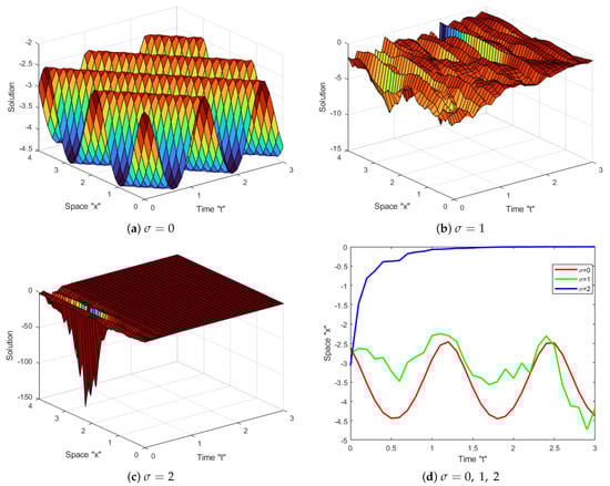
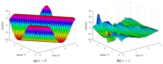
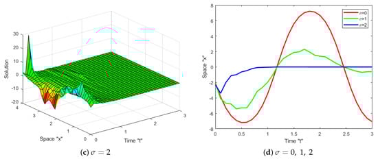
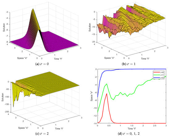
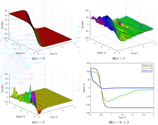
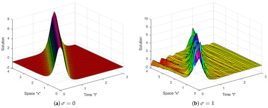
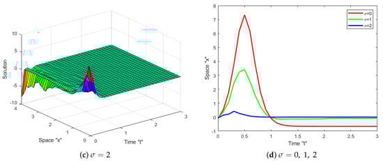
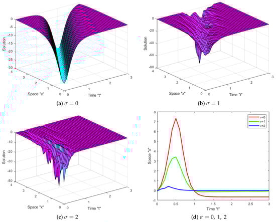
Impact of Noise: Now, let us investigate the impact of SWP on the exact solution of the coupled SKdV Equation (1). Several diagrams are given to clarify the behavior of some obtained solutions, such as (16)–(19), (34) and (35). Let us fix the parameters $x\in [0, 4]$ and $t\in [0, 3]$ to simulate these diagrams.

Now, we can notice from Figure 1, Figure 2, Figure 3, Figure 4, Figure 5 and Figure 6 that when the multiplicative noise is ignored (i.e., when $\sigma =0$), there are many other types of solutions, such as periodic solutions, kink solutions, and so on. After short transit patterns, the surface becomes flatter when noise is incorporated, and its amplitude is increased by $\sigma =1,2$. This demonstrates that SWP plays a significant role in shaping the behavior of the exact solutions of CSKdV equations and keeps them stable around zero, preventing the generation of rogue waves.

Figure 1. (a–c) display 3D style of solution $\Phi (x,t)$ in Equation (16) with $k=1.5$ and $\sigma =0,1,2$ (d) shows 2D style of Equation (16) with different $\sigma$.

Figure 2. (a–c) display 3D style of solution $\Psi (x,t)$ in Equation (17) with $k=1.5$ and $\sigma =0,1,2$ (d) shows 2D style of Equation (17) with different $\sigma$.

Figure 3. (a–c) display 3D style of solution $\Phi (x,t)$ in Equation (18) with $k=2$ and $\sigma =0,1,2$ (d) shows 2D style of Equation (18) with different $\sigma$.

Figure 4. (a–c) display 3D style of solution $\Psi (x,t)$ in Equation (19) with $k=2$ and $\sigma =0,1,2$ (d) shows 2D style of Equation (19) with different $\sigma$.

Figure 5. (a–c) display 3D style of solution $\Phi (x,t)$ in Equation (80) with $k=2$ and $\sigma =0,1,2$ (d) shows 2D style of Equation (80) with different $\sigma$.

Figure 6. (a–c) display 3D style of solution $\Psi (x,t)$ in Equation (81) with $k=2$ and $\sigma =0,1,2$ (d) shows 2D style of Equation (81) with different $\sigma$.

6. Conclusions

In this study, the CSKdV Equation (1) forced by the multiplicative Wiener process in the Itô sense is considered. Utilizing a mapping method, we able to obtain new trigonometric, rational, hyperbolic, and elliptic stochastic solutions. Also, we can apply other methods, such as the extended trial equation, Hirota bilinear method, complex hyperbolic-function method, $exp(-\phi )$-expansion method, and so on, to obtain some various solutions. These obtained solutions can be applied to the analysis of a wide variety of crucial physical phenomena because the coupled KdV equations have important applications in various fields of physics and engineering. Furthermore, the SWP impacts on the analytical solution of CSKdV Equation (1) are shown using MATLAB software. We establish that the Wiener process stabilizes the solutions at zero. In future work, we can find the exact solutions for other SPDEs with multiplicative color noise. Also, we can study coupled KdV equations with additive noise.

References

- Arnold, L. Random Dynamical Systems; Springer: Berlin/Heidelberg, Germany, 1998. [Google Scholar]
- Imkeller, P.; Monahan, A.H. Conceptual stochastic climate models. Stoch. Dyn. 2002, 2, 311–326. [Google Scholar] [CrossRef]
- Al-Askar, F.M.; Mohammed, W.W.; Aly, E.S.; EL-Morshedy, M. Exact solutions of the stochastic Maccari system forced by multiplicative noise. ZAMM J. Appl. Math. Mech. 2022, 103, e202100199. [Google Scholar] [CrossRef]
- Mohammed, W.W.; Al-Askar, F.M.; Cesarano, C. The analytical solutions of the stochastic mKdV equation via the mapping method. Mathematics 2022, 10, 4212. [Google Scholar] [CrossRef]
- Al-Askar, F.M.; Cesarano, C.; Mohammed, W.W. Multiplicative Brownian Motion stabilizes the exact stochastic Solutions of the Davey–Stewartson equations. Symmetry 2022, 14, 2176. [Google Scholar] [CrossRef]
- Al-Askar, F.M.; Cesarano, C.; Mohammed, W.W. The Solitary Solutions for the Stochastic Jimbo–Miwa Equation Perturbed by White Noise. Symmetry 2023, 15, 1153. [Google Scholar] [CrossRef]
- Mohammed, W.W.; Cesarano, C. The soliton solutions for the (4 + 1)-dimensional stochastic Fokas equation. Math. Methods Appl. Sci. 2023, 46, 7589–7597. [Google Scholar] [CrossRef]
- Wu, Y.T.; Geng, X.G.; Hu, X.B.; Zhu, S.M. A generalized Hirota-Satsuma coupled Korteweg-de Vries equation and Miura transformations. Phys. Lett. A 1999, 255, 259–264. [Google Scholar] [CrossRef]
- Inan, I.E. Exact solutions for coupled KdV equation and KdV equations. Phys. Lett. A 2007, 371, 90–95. [Google Scholar] [CrossRef]
- Zhou, Y.; Wang, M.; Wang, Y. Periodic wave solutions to a coupled KdV equations with variable coefficients. Phys. Lett. A 2003, 308, 31–36. [Google Scholar] [CrossRef]
- Fan, E.; Zhang, H. New exact solutions to a system of coupled KdV equations. Phys. Lett. A 1998, 245, 389–392. [Google Scholar] [CrossRef]
- Hon, Y.C.; Fan, E.G. A series of new exact solutions for a complex coupled KdV system. Chaos Solitons Fractals 2004, 19, 515–525. [Google Scholar] [CrossRef]
- Bhrawy, A.H.; Abdelkawy, M.A.; Kumar, S.; Johnson, S.; Biswas, A. Solitons and other solutions to quantum Zakharov–Kuznetsov equation in quantum magneto-plasmas. Indian J. Phys. 2013, 87, 455–463. [Google Scholar] [CrossRef]
Disclaimer/Publisher’s Note: The statements, opinions and data contained in all publications are solely those of the individual author(s) and contributor(s) and not of MDPI and/or the editor(s). MDPI and/or the editor(s) disclaim responsibility for any injury to people or property resulting from any ideas, methods, instructions or products referred to in the content. |
© 2023 by the authors. Licensee MDPI, Basel, Switzerland. This article is an open access article distributed under the terms and conditions of the Creative Commons Attribution (CC BY) license (https://creativecommons.org/licenses/by/4.0/).