1. Introduction
Rehabilitation robots have become an increasingly important area of research in recent years due to their potential to provide personalized and effective rehabilitation for individuals with mobility impairments resulting from neurological disorders such as stroke, spinal cord injury, or brain injury [
1,
2]. The development of rehabilitation robots offers a new approach to address the limitations of traditional rehabilitation methods. These robots can provide more intensive and repetitive training, which is essential for the formation of new neural pathways in the brain [
3,
4]. The importance of rehabilitation robots is underscored by their ability to address several challenges that traditional rehabilitation methods cannot adequately address. For example, they can provide customized and targeted training to specific areas of the body, which is difficult to achieve with traditional methods [
5,
6,
7]. Additionally, they can provide objective measurements of patient progress, allowing clinicians to monitor progress and adapt treatment regimens to meet individual needs [
8]. Also, rehabilitation robots can offer a safe and controlled environment for patients to exercise and recover, minimizing the risk of further injury [
9,
10].
Rehabilitation robots present a significant challenge for researchers due to their dynamic complexity. These systems involve numerous degrees of freedom and exhibit nonlinear and time-varying behaviors, which can make them difficult to model and control [
11]. Furthermore, they require real-time monitoring and control, which is essential for providing safe and effective rehabilitation. The complex nature of these systems also leads to challenges in identifying and predicting unknown dynamics, which can limit the effectiveness of control strategies [
12,
13]. In [
14], a new method has been introduced for identifying the dynamic parameters of robots with any number of degrees of freedom using Lie theory. Traditional methods have been perceived as cumbersome and have not been considered universally applicable. In this approach, the robot dynamics model has been represented as a matrix equation, having been reorganized from the Newton–Euler formula. With the use of the Kronecker product, important dynamics components like inertia tensors, masses, and friction coefficients have been extracted. The Kronecker–Sylvester identification equation has been presented as an optimization challenge and has been addressed using matrix techniques based on various joint data. Although such methods show promise, there is still room for improvement using new technologies. Hence, as technology continues to advance, the potential for rehabilitation robots to provide even more personalized and effective rehabilitation increases.
The presence of unknown dynamics in rehabilitation robots can negatively impact the performance of the system and lead to safety concerns for the patient. Therefore, the accurate identification and estimation of these disturbances are crucial for developing effective control strategies that can mitigate their effects [
15,
16]. Estimating the disturbances in rehabilitation robots can be challenging due to the complex and nonlinear nature of the system. The identification of disturbances typically involves developing mathematical models of the system and measuring the difference between the model prediction and actual behavior of the system [
17,
18]. However, in rehabilitation robots, it can be difficult to obtain accurate models due to the presence of uncertainties and unknown dynamics.
The importance of disturbance identification and estimation in rehabilitation robots cannot be overstated. The accurate identification and estimation of disturbances are crucial for ensuring safe and effective rehabilitation for patients. Despite the challenges, conventional techniques have been widely used to estimate and predict disturbances in rehabilitation robots. These techniques include adaptive control strategies [
19,
20], neural networks [
21,
22], and Kalman filters [
23,
24]. While these methods can help to improve the accuracy of disturbance estimation and lead to more effective control strategies that can adapt to the dynamic behavior of the system, it is important to note that most of the existing algorithms rely on conventional methods and do not incorporate state-of-the-art techniques. Therefore, there is still room for improvement in the field of disturbance estimation in rehabilitation robotics.
One of the state-of-the-art techniques that is barely used for identification in rehabilitation robots is the Gaussian process. Gaussian process regression is a powerful statistical technique that has shown promise in identifying and predicting unknown dynamics of complex systems [
25,
26]. This technique is particularly useful in systems where mathematical models are difficult to obtain due to uncertainties and nonlinearities. Gaussian process regression can model complex functions without assuming a specific functional form, making it well-suited for identifying unknown dynamics in rehabilitation robots. By modeling the system’s response to various inputs, Gaussian process regression can identify the unknown dynamics of the system and predict its behavior in response to new inputs.
The sampling process is a critical issue in the dynamic identification of rehabilitation systems, as obtaining accurate samples from the unknown dynamic of these systems is a challenging task. Consequently, most studies in this field treat the unknown dynamics of these systems as disturbances in control applications rather than identifying them [
27,
28]. However, with the advent of new techniques, it is possible to accurately estimate the unknown dynamics of these systems, and the resulting information can be used in the downstream tasks of these robots. Therefore, incorporating these advanced techniques in dynamic identification can potentially enhance the control and overall performance of rehabilitation robots.
Advancements in research and development in the area of rehabilitation robots hold great potential for enhancing patients’ quality of life. With the goal of contributing to this matter, our study proposes a novel algorithm that utilizes a finite-time estimator and Gaussian process to identify the unknown dynamics of rehabilitation robots. By developing more sophisticated and widely used rehabilitation robots, we can improve the effectiveness of rehabilitation treatments and enhance the overall well-being of patients. The proposed algorithm is a robust algorithm that takes samples of the model, and the accuracy of samples is guaranteed through the Lyapunov stability theorem. The use of finite-time observers in combination with Gaussian process regression further improves the accuracy of estimation by providing real-time estimates of the system’s state. Also, the proposed algorithm takes advantage of the probabilistic nature of Gaussian process regression in disturbance estimation for rehabilitation robots, which is a promising area of research that has the potential to significantly improve the accuracy and effectiveness of control strategies for these complex systems.
The structure of the current study is outlined as follows.
Section 2 provides an overview of the dynamical model used for a 2-DoF knee rehabilitation robot.
Section 3 presents a background on Gaussian processes to provide a comprehensive understanding of the methodology utilized in this study. Then in
Section 4, we propose a finite-time estimator and an identification algorithm based on finite-time sampling and a Gaussian process for the identification of the unknown dynamics of the rehabilitation robot. In
Section 5, we test the proposed algorithm in various scenarios and apply it to the system in combination with feedback linearization control to demonstrate its excellent performance. Finally,
Section 6 concludes the study by presenting our findings and future research directions.
2. Problem Formulation
The mathematical modeling of a rehabilitation robotic system consisting of
links is given by [
29]
Here,
represents the joint angles,
denotes the rate of change in these angles (joint velocities), and
signifies the acceleration of the joints. The terms
and
encapsulate the inertia of the robot and the combined centripetal and Coriolis forces, respectively. The vector
stands for the gravitational torques acting on the robot’s joints. On the other hand,
embodies the input torques that drive the robot’s motion. Additionally, the Jacobian matrix
links the joint velocities to the velocity of the robot’s end-effector. Lastly,
signifies the external forces applied to the robot, such as those from the user. This equation, grounded in standard robotic conventions, captures the intricate interplay of various forces and responses in a robotic system. It is noteworthy that the
matrix satisfies the conditions of symmetry [
30] and the dynamic equation’s left-hand side can be expressed as a linear parameterization:
where
is the vector of dynamic parameters of the system and
is the regression matrix, which contains unknown functions of the signals
, and
. It is assumed that the constrained force
is uniformly bounded. This assumption is deemed reasonable from an engineering standpoint since the time-varying constrained force
is expected to be bounded.
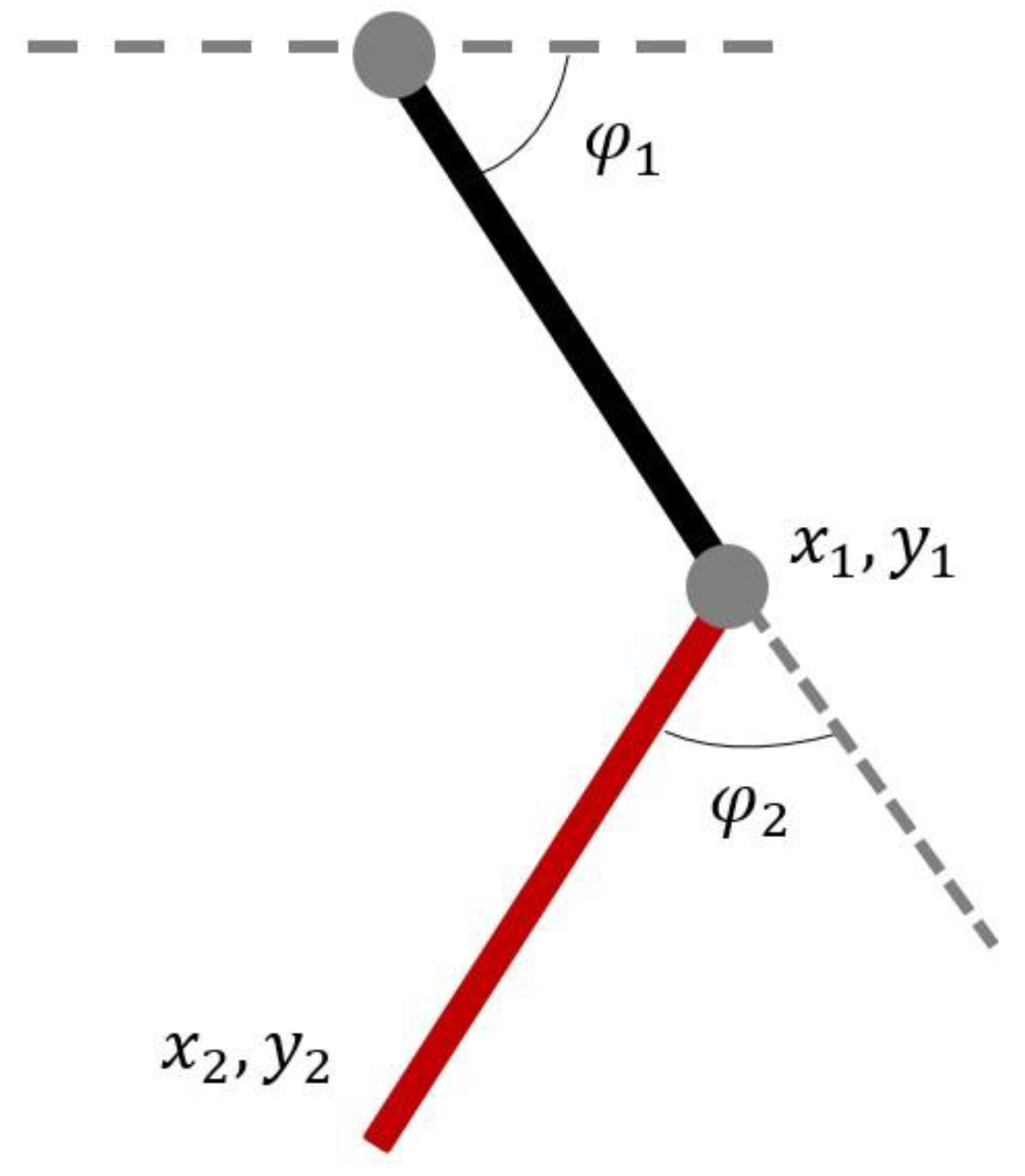
Figure 1 shows a 2-DoF knee rehabilitation robot with two revolute joints in the vertical plane. The system consists of a mechanical structure that resembles a human leg, with two degrees of freedom at the knee joint. Two motors actuate the joint through a transmission system that includes a ball screw and a timing belt. The motors are controlled by a computer, which receives feedback from sensors located at various points in the system. The sensors measure joint position, velocity, and acceleration, as well as motor torque and current. The computer calculates the desired torque inputs to achieve a desired trajectory and sends them to the motors.
To derive the equation of motion that yields the parameters of Equation (1), we utilize the Euler–Lagrange equations. We consider
as generalized coordinates. The kinetic energy can be expressed as:
where the distance between joint
and the center of mass of link
is represented by
. Furthermore,
denotes the moment of inertia of link
about an axis that extends out of the page and passes through the center of mass of link
, where
takes on values of 1 and 2. The potential energy is written as:
Using the Lagrange equation, the dynamic of the system is obtained by:
The kinematics of the robot and the Jacobian matrix are given by:
Remark 1. In evaluating robotic complexity, it is intuitive to assume that a 2-DoF robot offers fewer challenges than its 6-DoF counterpart. However, when contextualized within the domain of rehabilitation robotics, this perspective demands a more detailed interpretation by considering the following factors: (1) Direct human–robot interactions impose inherently unpredictable dynamics, necessitating rigorous safety protocols to mitigate potential harm. (2) The heterogeneity in individual human physiological responses compels the need for robots to possess extensive adaptability mechanisms. (3) Contrary to interfaces with rigid substrates, rehabilitation robots engage with the multifaceted dynamics of human soft tissues, muscles, and joints. (4) A concurrent challenge is the requisite integration with broader health-monitoring frameworks, introducing additional layers of operational complexity. Consequently, the intricacies inherent to a 2-DoF rehabilitation robot, given its symbiotic relation with human biomechanics, can arguably rival the complexities encountered in high-DoF industrial robotic applications.
3. Gaussian Processes
Simulators, which are frequently used to model intricate real-world phenomena in various fields of science and technology, often rely on mathematical models. However, these models can be computationally demanding due to the complexity of the systems being simulated. Emulators, which aim to construct a mathematical representation of these systems and processes, offer a potential solution to this problem. Among the methods used to create emulators, Gaussian processes are widely employed due to their effectiveness and popularity [
31,
32,
33].
3.1. Gaussian Processes Formulation
Data obtained from laboratory experiments or computer simulations may be subject to noise. This can result in variations in the input–output relation, which can be viewed as a single realization from a random process
:
In this context, the inputs in the training data are represented by vector
. The mean function is defined using a pre-determined set of basis functions and the unknown coefficient of the mean function which respectively are denoted by
and
. A zero-mean Gaussian process (
) is also involved, and its parametric covariance function is defined by
The variance of the process is denoted by
, and the correlation function is represented by
, where
, is a measure of similarity between
and
. Numerous correlation functions have been put forward in scholarly works; however, the Gaussian correlation function stands as the most frequently utilized one. This function can be expressed as follows:
The hyperparameters are denoted by
and
in which
is a scalar and
is a diagonal matrix. To perform Gaussian process modeling, the estimation of parameters
and
is essential. This can be performed through maximum likelihood estimation [
34,
35,
36]. Maximum likelihood estimation is a statistical method used to estimate the parameters of a model by maximizing the likelihood function. In the case of Gaussian process modeling, the multivariate Gaussian likelihood function is used. This function is defined as the probability density function of a multivariate Gaussian distribution, which is determined by the mean vector and the covariance matrix. The likelihood function is expressed as follows:
Using the natural logarithm represented by , the correlation matrix, with elements for , and the outputs of the training data are denoted by the vector . Also, is the matrix with the element .
In order to obtain an estimate of the hyperparameters
, and
, one can minimize Equation (10) using numerical optimization techniques. Many global optimization methods have been utilized for this purpose, such as particle swarm optimization, the genetic algorithm (GA), pattern searches, and gradient-based optimization [
37,
38,
39,
40,
41]. Nevertheless, gradient-based optimization methods are often the preferred choice for maximum likelihood estimation in Gaussian process models due to their computational efficiency and ability to efficiently optimize the many model parameters involved in these models.
Applying Gaussian process modeling enables us to obtain the mean and variance of the predicted probability distribution at any input point
. Specifically, the mean prediction is given by the posterior mean function, which is a linear combination of the training data with weights determined by the covariance between the training data and the test point. The variance of the prediction, on the other hand, is determined by the posterior covariance function, which measures the uncertainty in the prediction due to the noise in the data and the choice of the kernel function. The mean and variance of the prediction are respectively given by
where for each training data point
, we compute a value
, and collecting these values for all
training data points, we obtain a column vector
which measures the similarity of
with all training data. Also, using the similarity values between the training data points, we can construct a covariance matrix
, where the
element is given by
.
3.2. Comparison with Other Techniques
In the realm of algorithmic methodologies, GPs stand apart from techniques like neural networks, deep learning, particle swarm optimization (PSO), and genetic algorithms (GAs) not necessarily in novelty but in their foundational approaches and areas of applicability. While deep learning methods excel in tasks involving high-dimensional data and have revolutionized domains such as image processing, GPs, being non-parametric, offer a probabilistic lens to both supervised and unsupervised learning scenarios. Conversely, optimization strategies like PSO and GA shine in environments characterized by complex, non-continuous search spaces, where traditional gradient-based techniques might be inadequate.
The main benefits of Gaussian processes include (1) Interpretability: GPs inherently furnish an interpretative framework, elucidating uncertainties associated with predictions. (2) Data efficiency: owing to their probabilistic nature, GPs can render credible predictions with limited data, circumventing the voluminous data prerequisites often seen with deep architectures. (3) Optimization synergy: in contexts such as Bayesian optimization, the inherent uncertainty quantification of GPs renders them particularly effective. (4) Resilience to overfitting: with judicious kernel and hyperparameter selection, GPs demonstrate a reduced predisposition to overfit, especially in scenarios where data might be scarce.
4. The Proposed Identification Algorithm
In this section, we propose a finite-time estimator for the rehabilitation robot and prove its convergence based on the Lyapunov stability theory. Then, we introduce our algorithm to identify the time-varying unknown dynamics of the rehabilitation robot.
4.1. Finite-Time Estimator
To reformulate the equation of motion of a multi-input multi-output rehabilitation robot with 2-DoF in the state space form, we define
=
and
=
as
, and the robot dynamics can be described as follows:
in which, based on Equation (1), one can obtain:
To account for both the uncertain terms of the system and the unknown dynamic as a single term, we use which should be estimated.
Lemmas 1 and 2 are utilized to introduce the finite-time estimator for the nonlinear rehabilitation robot.
Lemma 1. Consider a continuously differentiable positive definite function that satisfies the following inequality: Given that , and > 0 while , the function exhibits convergence to the equilibrium point within a finite time duration.
Lemma 2. The triangle inequality holds if and > 0 for then: In order to develop a finite-time estimator for the rehabilitation robot, we introduce the following auxiliary variables: where the variable is defined as follows: The variable is expressed using the design parameters , which are positive, and is greater than the 1-norm of vector , denoted as . Here, the symbol ‖.‖ represents the 1-norm. Additionally, we have odd positive integers and , where is less than . The estimated value of the uncertain dynamic (
)
is then determined as follows:
By taking into account Equations (13), (18), and (19), we arrive at the following equation: Based on Equations (13), (20), and (21), we obtain:
Theorem 1. By applying the proposed estimator, defined by Equations (18)–(20), to the MIMO uncertain nonlinear system expressed by Equation (14), the error of estimation, denoted by the variable , converges to zero within a finite time.
Proof. Let us consider the positive definite Lyapunov function candidate as follows:
The time derivative of the function
can be expressed as:
Lemma 3 was used to derive the final line of Equation (24).
Lemma 3. Taking the following functionthe following equation is obtained As we know =
, we obtain the following as a result: Accordingly, the finite-time convergence of the estimation error to zero has been proven for the proposed disturbance estimator using Lemmas 1, 2, and 3 along with Equation (27), which satisfies the Lyapunov condition. □
4.2. The Algorithm
In the previous section, we discussed the use of Gaussian processes to predict the value of dynamic uncertainties in rehabilitation robots. However, there is a significant challenge in obtaining samples from these uncertainties and unknown dynamics in reality. This challenge must be addressed in order to make any meta-modeling technique like Gaussian processes or neural networks practical in real-world applications.
For rehabilitation robots, we have inputs and outputs, and if we design the system’s states in an observable manner, we can obtain the system’s states as well. However, these meta-modeling techniques can only model the relationship between the given input and output and cannot model a part of the system. Furthermore, they only work perfectly under ideal conditions. This is a major obstacle and an open question in the field of robotics and identification. To address this challenge, we propose a Gaussian process based on a finite-time estimator. We propose a finite-time estimator and prove its finite-time convergence using the Lyapunov theorem. As delineated in
Section 3.1, we define the estimator to only identify the unknown and unmodeled dynamics. Then, using the samples and information obtained from the estimator, we fit a Gaussian process and model the unknown dynamics of the system.
The strength of our model lies in its finite-time guaranteed convergence, which ensures the existence of trustworthy samples for the Gaussian process. In summary, our approach uses a Gaussian process based on a finite-time estimator to model the unknown and unmodeled dynamics of rehabilitation robots. Our method provides trustworthy samples for the Gaussian process, ensuring practical applicability in real-world settings. Our approach addresses an open question in the field of robotics and identification and contributes to the development of rehabilitation robots.
4.3. Feedback Linearization Augmented by the Proposed Algorithm
In this part, we provide feedback linearization control for rehabilitation robots augmented by our proposed approach. By integrating a robust estimator with feedback linearization, we are essentially combining model-based control with model-free learning, aiming for the best of both worlds.
Using feedback linearization, the control objective is to cancel out the nonlinearities and derive a control input
to stabilize the system. The system dynamics are presented in Equations (13)–(15), where
is estimated using the proposed algorithms as
and represents the uncertain and unknown dynamics. To linearize the system, we define the control input
as:
here
is the auxiliary control input which will be designed to stabilize the linearized system. Inserting this into the system dynamics, we obtain:
which resembles a double integrator system. A common choice for
in the feedback linearization technique is:
where
and
are positive constants. To prove stability, we can use a Lyapunov function. A common choice for a double integrator system is:
Taking its time derivative:
Theorem 1 guarantees the fact that the estimation error
converges to zero in a finite time. Therefore, after a finite time we have
Inserting the proposed control law in Equation (33), we have:
This derivative is negative definite, implying that the origin is stable and the system asymptotically converges to it.
4.4. Details for Implementing the Proposed Algorithm
The process initiates with the acquisition of electromyographic (EMG) signals. These signals are captured using advanced EMG sensors, which are part of a comprehensive data acquisition system specifically designed for biomechanical applications. The sensors are strategically positioned on the lower limb to ensure optimal signal capture. The positioning takes into account muscle groups of primary interest, and the sensors are usually attached to the skin using hypoallergenic adhesive pads to maintain stable contact throughout the procedure.
To ensure the fidelity of the captured signals, the data acquisition system is equipped with high-resolution analog-to-digital converters and signal filtering mechanisms, and it is synchronized with a computer interface for real-time data visualization and storage. This setup not only guarantees accurate data collection but also enables immediate feedback and calibration if required.
Once these EMG signals are acquired and pre-processed, they are sent to a meticulously calibrated transformer. This transformer converts the EMG signals into the desired positions to which the rehabilitation robot’s limbs should navigate. Following this transformation phase, a controller—outfitted with the proposed identifier—actively drives the links of the robotic system to align with these predetermined desired values. This methodology ensures precision and ease of application, and it optimizes the robot’s performance in rehabilitation contexts.
5. Numerical Results
In this section, we evaluate the effectiveness of the proposed algorithm through three different examples. Specifically, in Examples 1 and 2, we illustrate the performance of the proposed method in the identification of the unknown complex dynamics of the system. In Example 3, we utilize the information obtained from the algorithm for control purposes.
5.1. Identifying Time-Varying Continuous Dynamic
In this example, we aim to investigate the effectiveness of the proposed algorithm in estimating the unknown dynamics of a system. Specifically, the unknown dynamic is given by:
where
is the constrained force exerted by the user and
is the Jacobian matrix of the system and is defined in Equation (6).
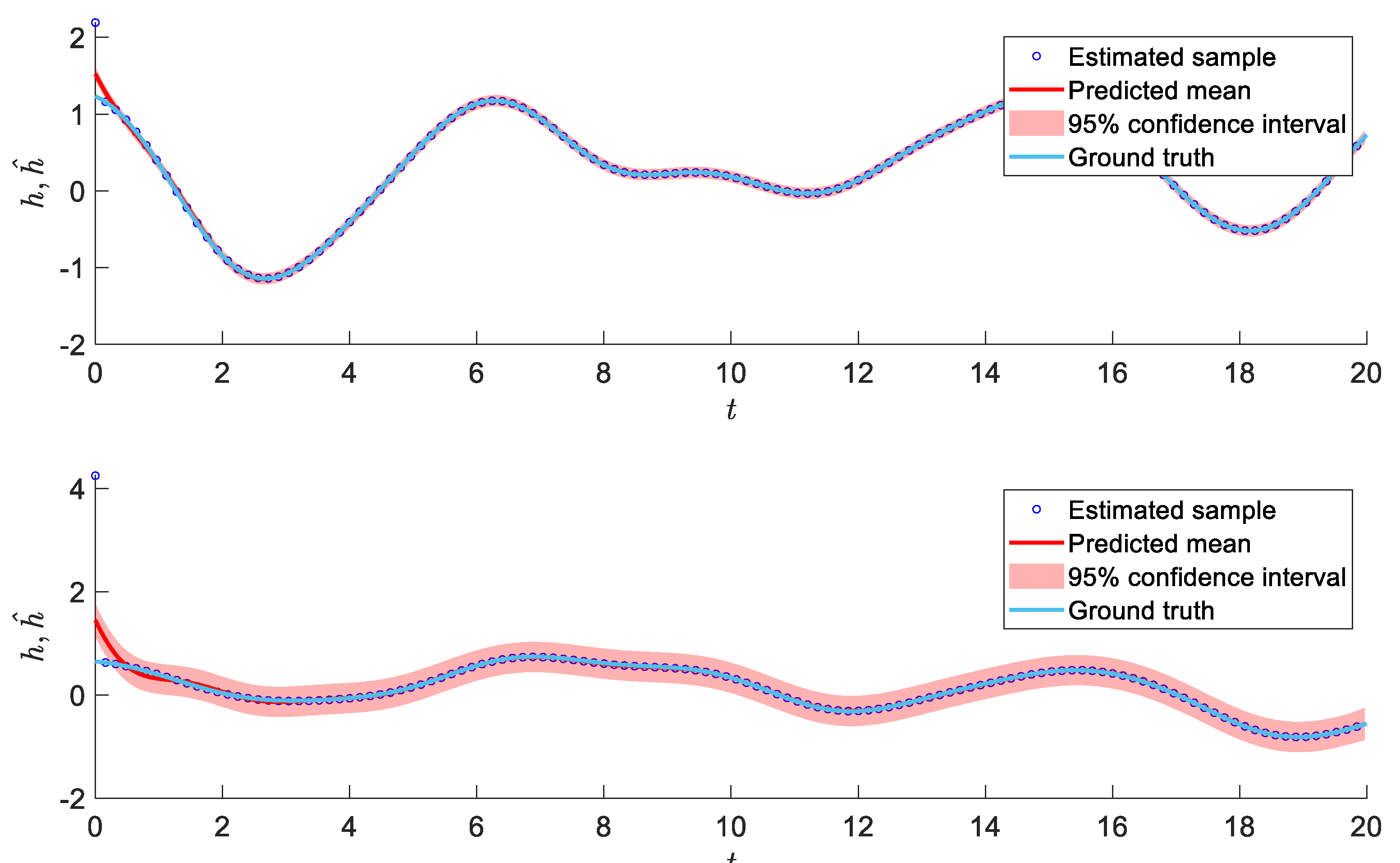
Figure 2 and
Figure 3 depict the states of the system and the applied torque of the rehabilitation robot under the proposed algorithm. As shown in
Figure 2, the proposed finite-time estimator extracted accurate samples and the Gaussian process was able to learn the complex unknown dynamics effectively, and its performance in predicting the test set was remarkable. Also,
Figure 3 demonstrates that the applied torque remains within a practical range, which guarantees the effectiveness of the proposed method. Therefore, it is evident that the proposed algorithm can efficiently enhance the down-stream tasks in rehabilitation robots.
It is noteworthy that despite the presence of noise in the estimated data, the Gaussian process successfully eliminated the noise and yielded precise data predictions. Notably, the outcomes demonstrate an excellent agreement with the actual value of the unknown dynamic of the systems, as evidenced by the close alignment between the red line and the blue line in
Figure 2. An additional benefit of the proposed algorithm is the uncertainty bounds provided by Gaussian processes. These bounds can be highly advantageous in the design of controllers and the determination of their stable ranges for system parameters. The estimated uncertainties can help to address the challenge of determining the stability range for system control in practice.
5.2. Identifying Time-Varying Discontinuous Dynamic
Traditional methods have difficulty in identifying discontinuous dynamics that involve sudden changes, but our proposed method can handle such dynamics due to its probabilistic nature. This makes it possible to accurately predict unknown dynamic functions that are not possible to identify using traditional methods. To further demonstrate the effectiveness of our proposed algorithm, we consider an example with a discontinuous unknown dynamic function as follows:
where the
function generates discontinuous signals which are hard to estimate.
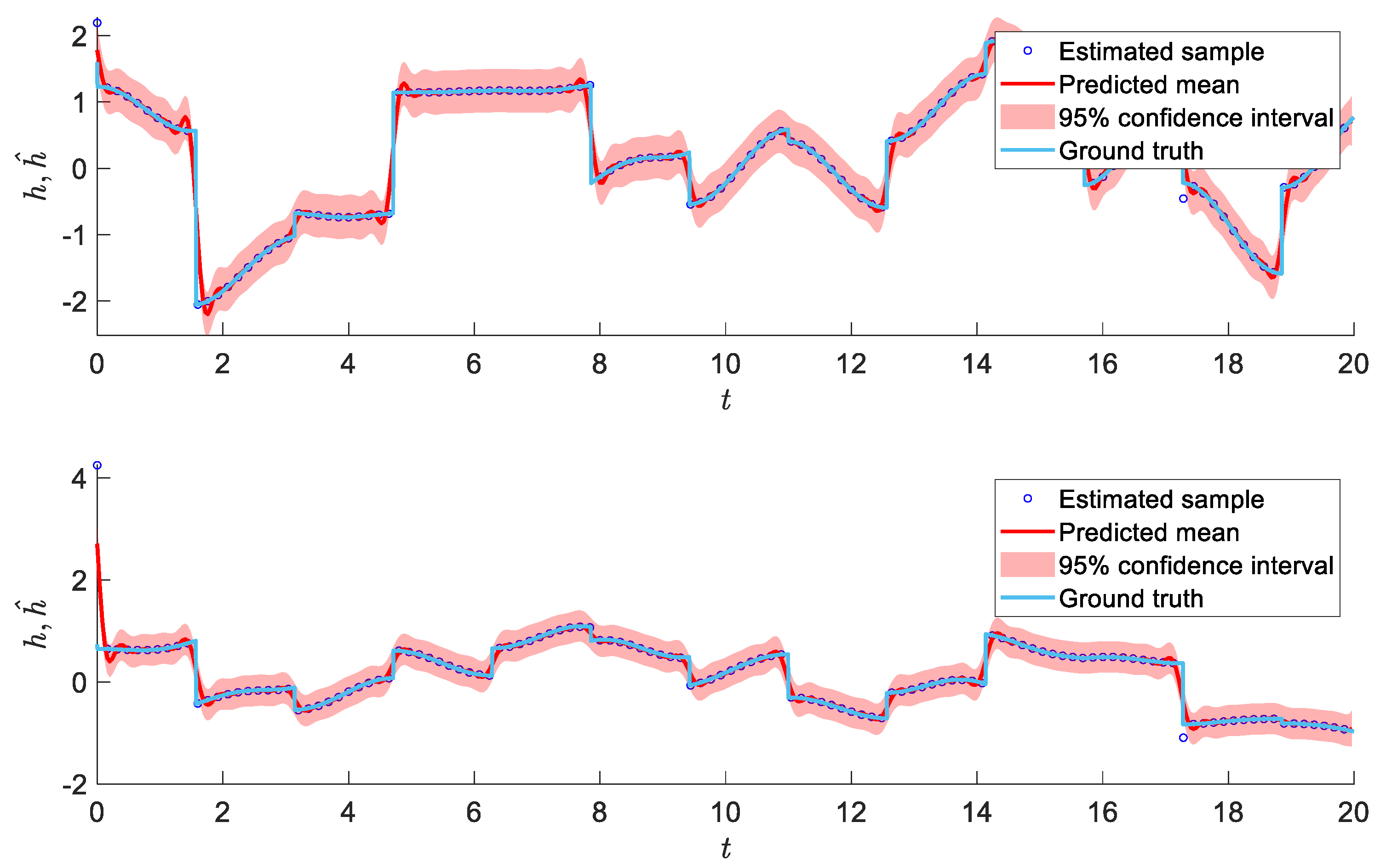
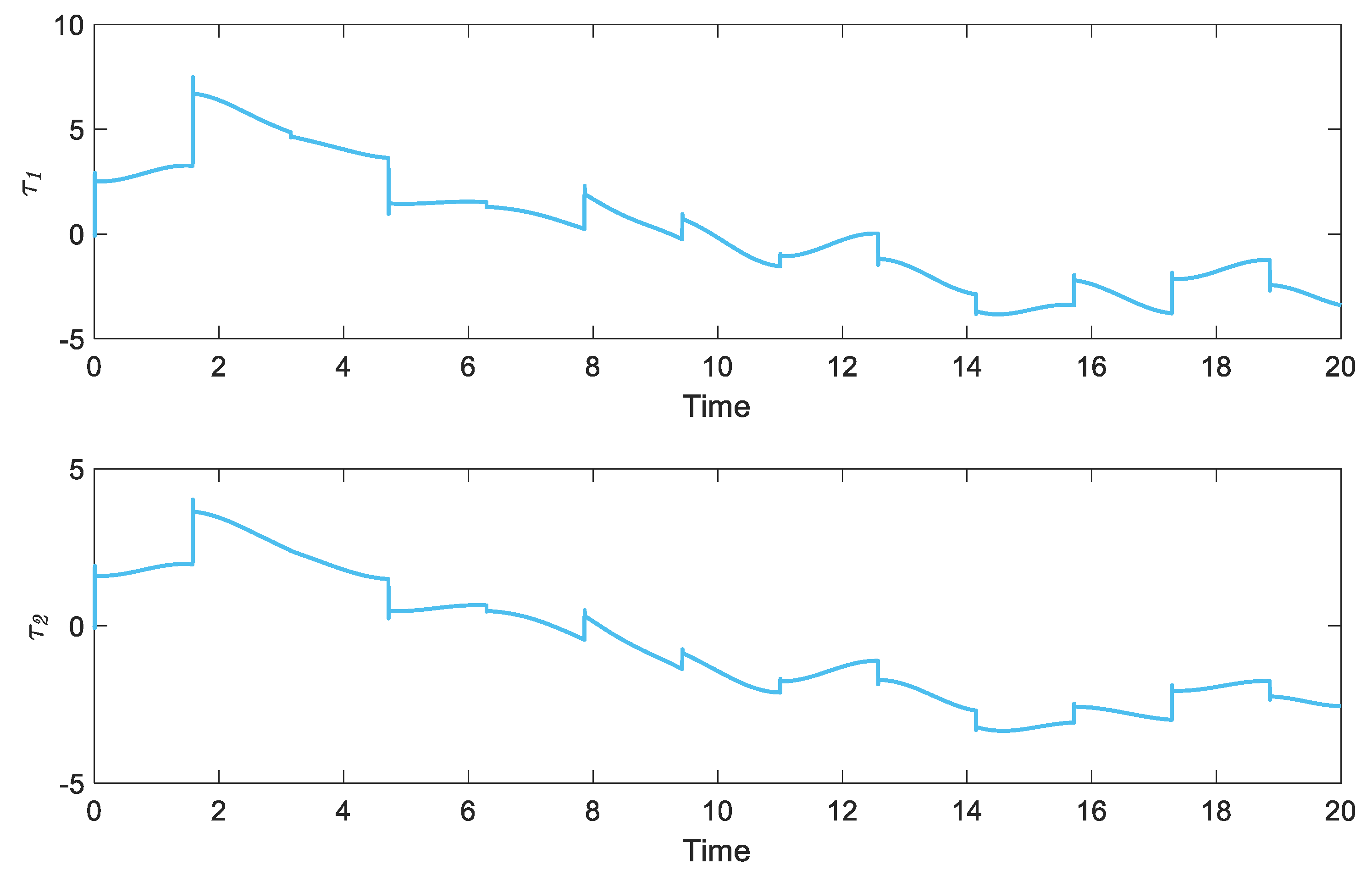
Figure 4 and
Figure 5 show the identification results and applied torque to the system. The results presented in
Figure 4 highlight the outstanding performance of the proposed algorithm in dynamic identification. Despite the highly discontinuous nature of the unknown dynamic, characterized by sudden changes resulting from the sign function, the proposed algorithm demonstrated an exceptional ability to learn the system’s complex and unknown dynamics accurately.
Moreover, the ability of the algorithm to maintain the system states and applied torque within practical ranges further highlights its effectiveness. The fact that the algorithm was able to achieve such accurate identification and prediction even in the presence of complex and variable dynamics is a testament to its robustness and reliability.
5.3. Using Identified Dynamic for Control of the Rehabilitation Robot
Now, we use the information obtained from the proposed algorithm and apply a feedback linearization controller to control the system. In light of the challenges posed by uncertainties, the suitability of a feedback linearization controller for controlling rehabilitation robots may be compromised. However, thanks to the effectiveness of the proposed algorithm in accurately estimating uncertainties, as demonstrated in the previous examples, we can now confidently apply the feedback linearization controller to the rehabilitation robot. By leveraging the precise estimation of uncertainties provided by the algorithm, we can harness the benefits of the feedback linearization controller, enabling an improved control performance in the presence of uncertainties.
The proposed feedback linearization control discussed in
Section 4.3 is applied with
and
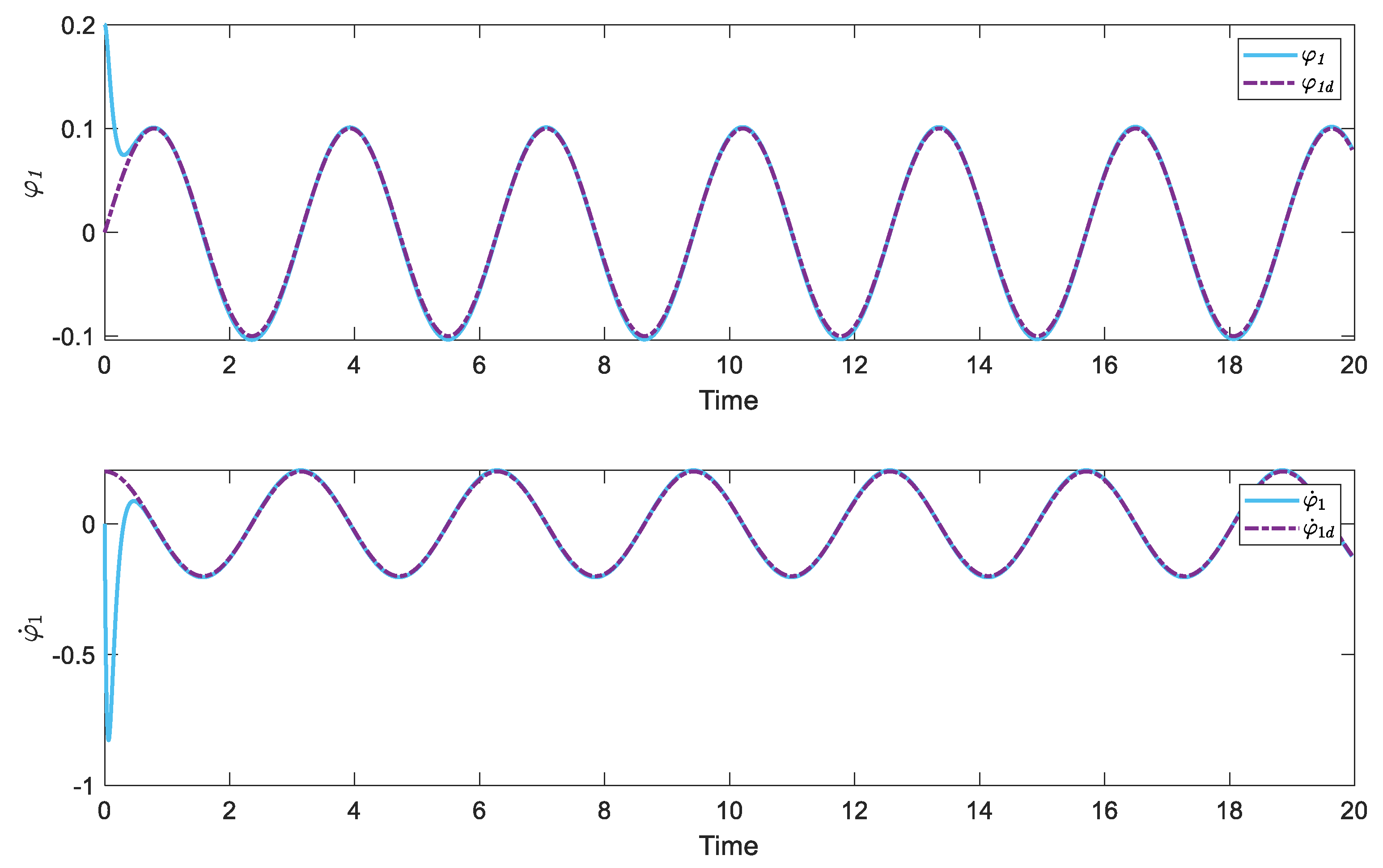
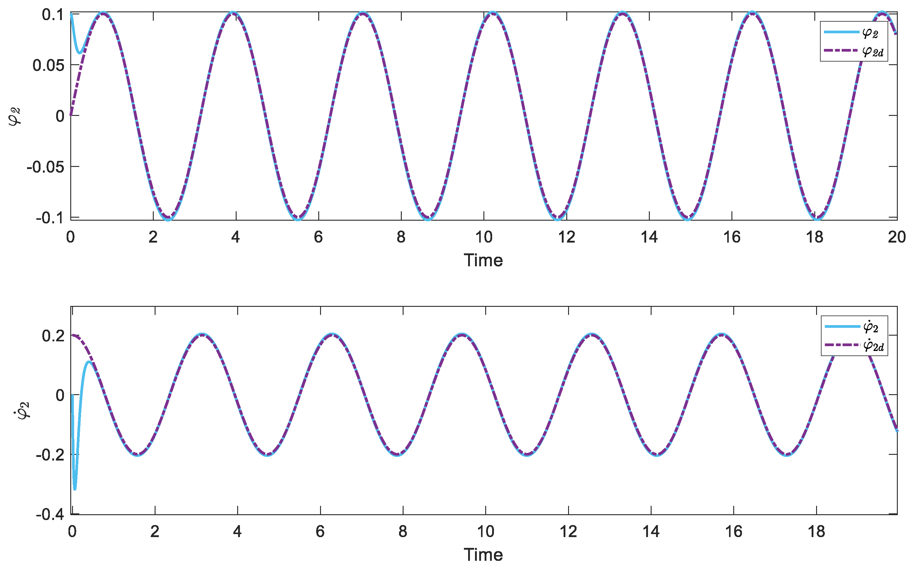
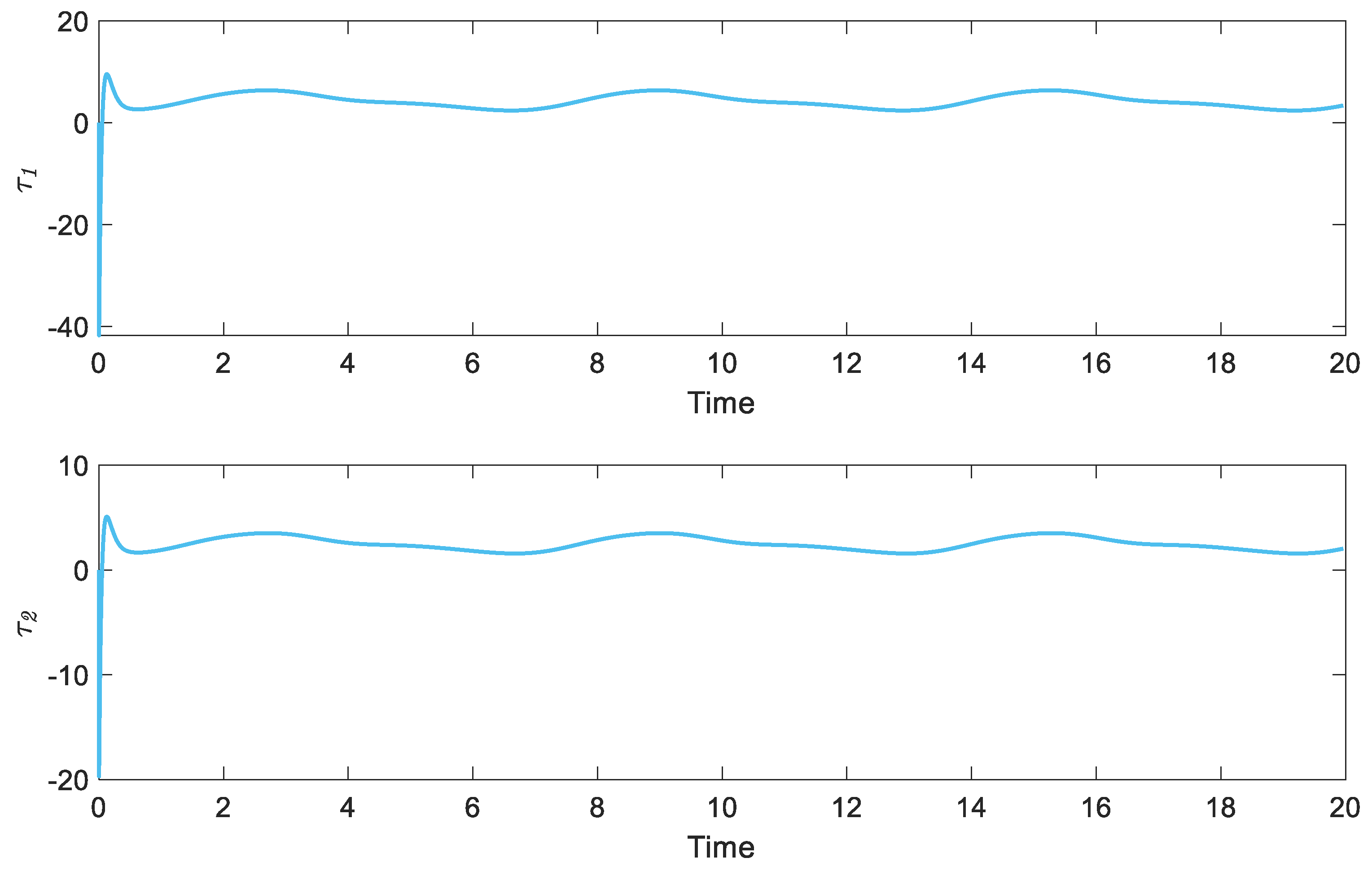
. The unknown dynamic of the system here is considered the same as Equation (28), and the identified dynamic using the proposed algorithm is used in the feedback linearization control. We consider the following desired trajectories.
Figure 6 and
Figure 7 depict the state of the system. Despite the considerable unknown dynamic in the control of the system, the proposed algorithm provides crucial information that enables feedback realization control to rapidly drive the system’s states toward the desired values. In addition,
Figure 8 illustrates the applied control torque, which exhibits an appropriate bound. Overall, the study’s outcomes provide compelling evidence that the proposed algorithm is remarkably efficient in identifying and predicting variable orders in the rehabilitation system, which makes it a valuable tool for developing advanced control strategies for this system.
6. Conclusions
In this study, we introduced a novel method for identifying the unknown dynamic of rehabilitation robots. Our proposed algorithm is a combination of finite-time estimators and a Gaussian process, which takes advantage of the probabilistic strength of Gaussian processes. We present the mathematical equations of a 2-DoF knee rehabilitation robot. Then, the proposed algorithm is presented and the accuracy of the sampling process is guaranteed using the Lyapunov theorem. After that, the proposed algorithm is applied to a 2-DoF knee rehabilitation robotic through three different examples. We illustrate the performance of the proposed method in identifying continuous and discontinuous unknown dynamics. The numerical results demonstrate that the proposed algorithm is able to handle both continuous and discontinuous unknown dynamics effectively, indicating the potential for this approach to be applied in various rehabilitation settings. Finally, we utilize the information obtained from the proposed algorithm for feedback linearization control. The numerical results of our study provide clear evidence of the excellent performance of our proposed algorithm. Overall, our approach has a great potential to significantly improve the performance of rehabilitation technologies, ultimately improving patient outcomes and quality of life. In control systems, uncertainty bounds are crucial for stability. Our GP-based framework offers these bounds, which are key for enhanced control. To continue advancing this field, we plan to leverage these bounds in our future work. Furthermore, the proposed method can be implemented in an experimental setup.
