Article

Motion-Tracking Control of Mobile Manipulation Robotic Systems Using Artificial Neural Networks for Manufacturing Applications

by
Daniel Galvan-Perez
1,
Francisco Beltran-Carbajal
2,*,
Ivan Rivas-Cambero
1,
Hugo Yañez-Badillo
3,
Antonio Favela-Contreras
4 and
Ruben Tapia-Olvera
5
1
Departamento de Posgrado, Universidad Politécnica de Tulancingo, Tulancingo de Bravo 43629, Mexico
2
Departamento de Energía, Universidad Autónoma Metropolitana, Unidad Azcapotzalco, Mexico City 02200, Mexico
3
Departamento de Investigación, TecNM—Tecnológico de Estudios Superiores de Tianguistenco, Tianguistenco 52650, Mexico
4
Tecnologico de Monterrey, School of Engineering and Sciences, Monterrey 64849, Mexico
5
Departamento de Energía Eléctrica, Universidad Nacional Autónoma de México, Mexico City 04510, Mexico
*
Author to whom correspondence should be addressed.
Mathematics 2023, 11(16), 3489; https://doi.org/10.3390/math11163489
Submission received: 25 June 2023 / Revised: 8 August 2023 / Accepted: 9 August 2023 / Published: 12 August 2023

Abstract

:
Robotic systems have experienced exponential growth in their utilization for manufacturing applications over recent decades. Control systems responsible for executing desired robot motion planning face increasingly stringent performance requirements. These demands encompass high precision, efficiency, stability, robustness, ease of use, and simplicity of the user interface. Furthermore, diverse modern manufacturing applications primarily employ robotic systems within disturbed operating scenarios. This paper presents a novel neural motion-tracking control scheme for mobile manipulation robotic systems. Dynamic position output error feedback and B–Spline artificial neural networks are integrated in the design process of the introduced adaptive robust control strategy to perform efficient and robust tracking of motion-planning trajectories in robotic systems. Integration of artificial neural networks demonstrates performance improvements in the control scheme while effectively addressing common issues encountered in manufacturing environments. Parametric uncertainty, unmodeled dynamics, and unknown disturbance torque terms represent some adverse influences to be compensated for by the robust control scheme. Several case studies prove the robustness of the adaptive neural control scheme in highly coupled nonlinear six-degree-of-freedom mobile manipulation robotic systems. Case studies provide valuable insights and validate the efficacy of the proposed adaptive multivariable control scheme in manufacturing applications.

1. Introduction

The robotics industry has experienced unprecedented growth in recent decades, transforming manufacturing operations completely [1,2,3]. Mobile manipulation robotic systems have emerged as efficient and versatile tools for automating various tasks in industrial environments [4,5,6]. This progress, however, has presented challenges in controlling the motion of robotic systems in manufacturing applications that require high levels of precision and reliability [7]. The need for enhanced accuracy in robotics comes from the requirement for precise manipulation of objects in manufacturing scenarios [8]. Accurately planned motion-tracking control represents a crucial part in ensuring the efficiency and quality of manufacturing operations [9,10,11]. As performance requirements become increasingly demanding—with stability, operating velocity, and high precision in tracking of motion profiles required in manufacturing operations—significant challenges arise in the design of advanced motion control systems [12]. Controlling robotic systems spans a broad spectrum, including complex assembly [13] and laser-based manufacturing [14]. Control systems must accurately orchestrate robot motions to ensure skillful performance. Precision is essential for tasks that demand intricate maneuvers and precise positioning [15,16,17]. In scenarios where speed and efficiency are imperative, high-velocity capabilities become equally crucial [18]. The robot’s ability to swiftly execute tasks and maneuver can significantly impact the productivity and cycle times of the overall manufacturing processes [19].
Improving a robotic system’s velocity and trajectory planning contributes to streamlined operations and production efficiency [20]. Nevertheless, achieving precise control and high velocity is one of many performance metrics for robotic systems, which depend on the specific application criteria of every sector. In addition, stability during operation is vital to maintaining the robot’s balance and prevent oscillations or disturbances that could compromise performance and safety, especially during tasks where the robot interacts with its environment or handles delicate objects [21,22,23]. Ensuring stability in front of parameter uncertainty, unmodeled dynamics, and unknown disturbance torques allows the system to operate efficiently, minimizing the risk of accidents or disruptions in the manufacturing process [24]. Designing control systems to meet manufacturing applications’ demanding precision, velocity, and stability requirements is complex. The challenge lies in integrating these three essential aspects and addressing the issues encountered in manufacturing environments, including parametric uncertainty, unmodeled dynamics, and disturbance torques [25,26,27]. Disturbances might introduce errors in motion-reference trajectory tracking. Deviations from desired trajectories and paths due to uncertainties in system parameters can negatively affect the overall performance of the robotic system as well.
Mobile manipulation robotic systems combine the manipulation dexterity provided by fixed-base manipulator robots with the mobility of mobile robots [28]. As a result, these coupled systems can perform complex tasks in changing environments, making them ideal for use in various applications, from manipulating objects in space [29] to factory automation [6] and home care [30]. Based on this, and considering the requirements of a robotic control system listed previously, it is necessary to highlight that mobile manipulation robotic systems must have precise and reliable motion control to achieve tasks effectively [13]. Therefore, motion-tracking control schemes are essential to ensure that mobile manipulator robots perform their assignments efficiently and safely [31]. Furthermore, the ability to control and adjust their position and velocity in real-time is essential to complete precise and complex duties involving manipulating objects and following predefined trajectories. In addition, motion-control schemes are also essential to ensure the stability and safety of mobile manipulation robotic systems, especially in dynamic and cluttered environments [32].
In light of numerous research developments addressing the efficient motion-control problem of mobile manipulation robotic systems, various perspectives have come to the fore. Ref. [33] offers a resolution for the motion control of a mobile manipulation system based on a two-stage algorithm to describe system motion in two phases. It utilizes a nonlinear control scheme grounded in Lyapunov theory. Ref. [34] introduces an approach centered on decentralized control for tracking the motion of a mobile manipulator in Cartesian space. The approach organizes the dynamic model into two interlinked subsystems and formulates separate kinematic controllers for the mobile and manipulator subsystems. Ref. [35] introduces a control scheme for a nonholonomic mobile manipulation framework with disturbances and unknown inertia parameters. The scheme uses an adaptive sliding mode control with parameter evaluation to ensure that the system follows the references without vibrations and with a quick convergence time to equilibrium. Ref. [36] presents a nonlinear robust control strategy incorporating an uncertainty estimator to manage the position tracking of a mobile manipulator in its task space. The scheme includes a feedforward control component to enhance control actions using the desired acceleration vector; a disturbance predictor to offset unfamiliar environmental factors such as parametric uncertainty, external disturbances, and unmodeled dynamics; and a decentralized PID controller within a feedback loop to enhance system stability. Ref. [37] unveils a control technique for mobile manipulators leveraging a fuzzy neural network and a Kalman filter for trajectory tracking. The study underscores the application of a fuzzy neural network to produce a feedforward torque while utilizing the Kalman filter to boost the computational effectiveness and precision of the learning algorithm. Ref. [38] outlines the application of an adaptable tracking control scheme for a nonholonomic mobile manipulator robot leveraging a hybrid PID approach. The control strategy comprises a conventional PID method with online self-teaching for adjusting the controller gains, an adaptive fuzzy neural network estimator, an adaptive robust controller-type compensator, and an adaptable control technique that takes into account the nonholonomic constraint force stability of the robotic system. Ref. [39] introduces a framework that enables a mobile manipulator to learn from human demonstrations, adapting to varied production and processing tasks in an unstructured environment. The approach comprises high-level path learning and low-level trajectory tracking control. Ref. [40] presents a trajectory tracking control structure for nonholonomic mobile manipulators with full-output limitations, where a velocity observer is described.
Furthermore, artificial intelligence has emerged as a transformative force in the manufacturing sector [41,42,43], primarily through its integration with controlled advanced robotic systems [44,45,46]. Particular emphasis is placed on applying intelligent control methods to robotic systems [47,48,49]. Central to this approach are artificial neural networks [50], which serve as a conduit between machine learning and deep learning [51]. Incorporating artificial neural networks into motion control of robotic systems can improve the efficiency, robustness, and adaptability of these systems, particularly in dynamic environments characterized by high complexity [52]. Artificial neural networks can be an excellent choice for enhancing the effectiveness of motion-control schemes for robotic systems [53]. Further, they offer numerous advantages, such as their ability to approximate mathematical models [54], robustness against disturbances [55], machine learning capabilities [56], ability to handle uncertainty [57], and reduced computational costs for identification and control applications [58]. B-Spline artificial neural networks been applied in this context and embody significant advancements in motion control of robotic systems such as aerial quadrotor robots [59,60,61] and anthropomorphic manipulator robots [62]. B-Spline artificial neural networks have also been exploited to derive control techniques for different types of electric motors like induction motors [63], DC shunt motors [64], and switched reluctance motors [65]. B-Spline artificial neural networks have been incorporated in controllers of electric power systems as well [66]. Robust trajectory tracking control of electromagnetic suspension represents another novel application of B-Spline artificial neural networks [67]. Nonetheless, there is no evidence of previous direct implementation of B-Spline artificial neural networks to control mobile manipulation robotic systems with high-precision motion-planning–trajectory-tracking requirements under substantially disturbed scenarios.
This paper introduces a novel adaptive neural robust dynamic control scheme to efficiently perform desired motion-planning–trajectory-tracking tasks for an important class of multi-input–multi-output nonlinear mobile manipulation robotic systems under significant disturbing influences in manufacturing applications. In contrast to other important control design methodologies, B-Spline artificial neural networks are capitalized to substantially improve the efficiency and robustness of robotic system control for a wide spectrum of uncertain disturbances. The main motivation for the inclusion of B-Spline artificial neural networks in the control scheme is to enhance its adaptive capability to compensate for parametric uncertainties, variable exogenous disturbances, and unmodeled dynamics using information about the position reference trajectory tracking error only. Dependence on detailed and accurate complex nonlinear mathematical modeling of the mobile manipulation robotic system is reduced in this fashion. Control parameters are tuned online according to operational conditions of the nonlinear robotic system. High-gain control actions that could lead to performance degradation and system instability are intelligently avoided. Moreover, different from other robust control techniques, asymptotic velocity observers as well as accurate real-time estimation of several types of uncertainties and disturbances on uncertain nonlinear dynamic systems are not required in the presented different control design perspective. Several case studies are developed to highlight the achieved robustness of the motion-tracking control scheme in highly coupled nonlinear six-degree-of-freedom mobile manipulation robotic systems. The case studies provide valuable insights and validate the efficacy of the control scheme in manufacturing applications.
A brief overview of the manuscript is as follows. A simplified mathematical representation of six-degree-of-freedom nonlinear mobile manipulation robotic systems for analysis and design of adaptive robust control is described in Section 2. A robust output feedback multivariable control approach for nonlinear mobile manipulation robotic systems is presented in Section 3. B-Spline artificial neural networks are then incorporated in the adaptive control scheme as described in Section 4. Tracking control efficacy of a considerably disturbed nonlinear mobile manipulation robotic system is highlighted in Section 5. Several numerical simulation experiments are developed to spotlight the neural control robustness capability. Finally, the conclusions in Section 6 provide critical findings and noteworthy observations.

2. Mathematical Modeling of the Mobile Manipulation Robotic System

The combination of a fixed-base manipulator robot and a mobile robot notably amplifies its skill. When functioning together, these robots can combine locomotion and manipulation, surpassing the mobility and operation limitations encountered when operating independently. A mathematical model that describes the kinematic and dynamic behavior of the robotic system is described in this section.

2.1. System Description

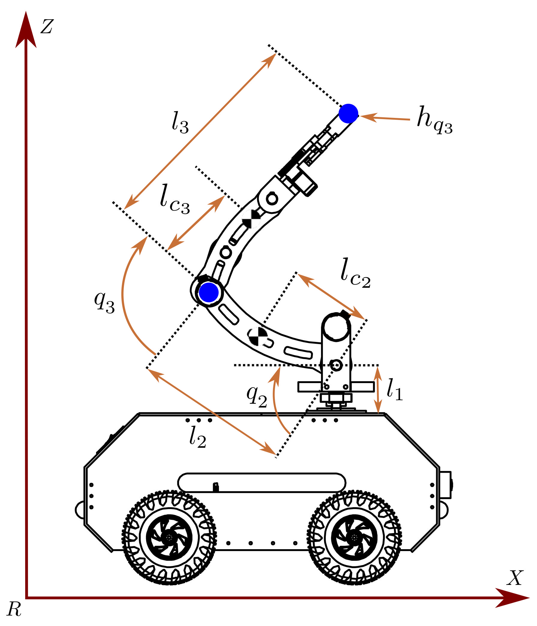
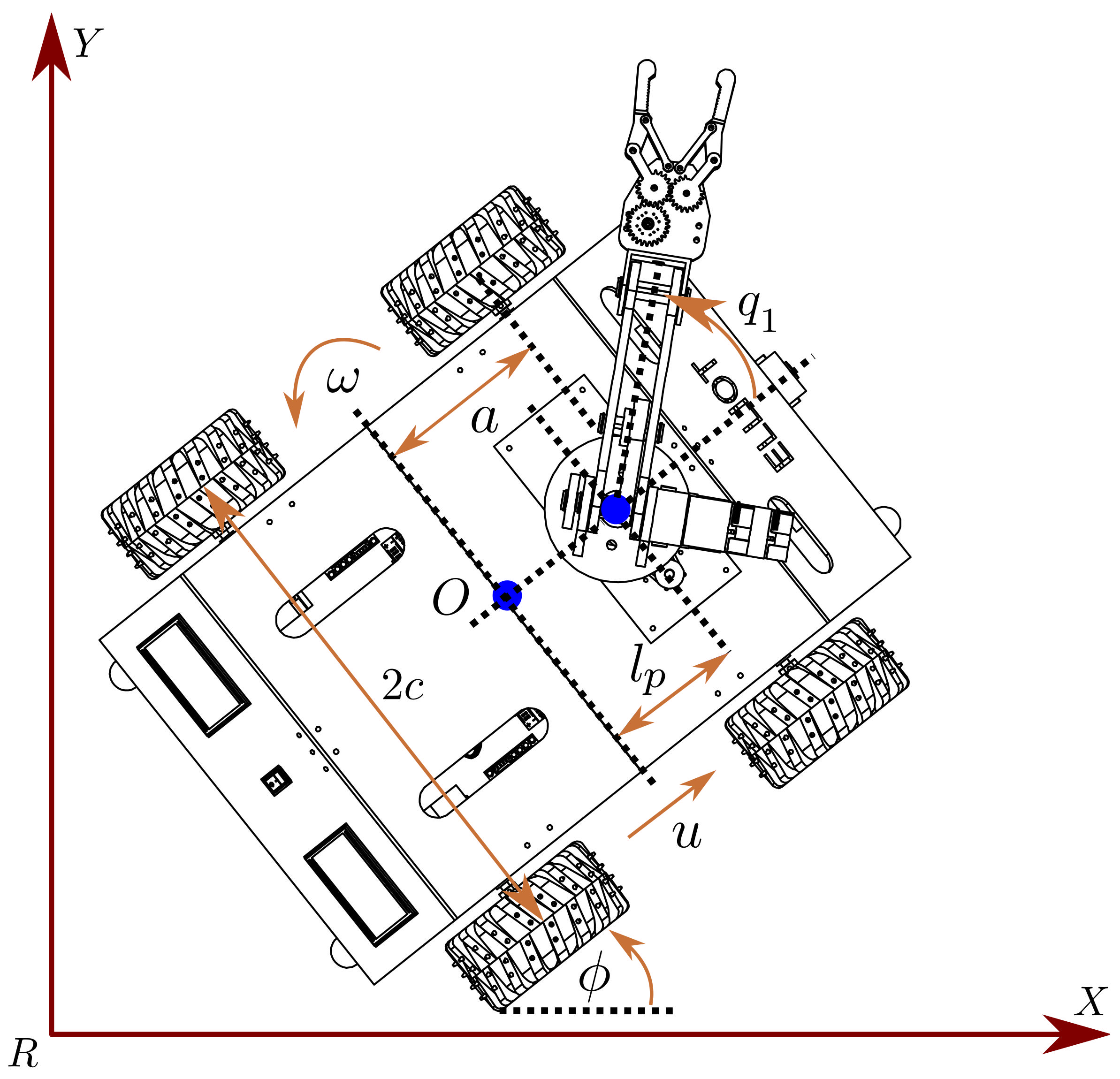
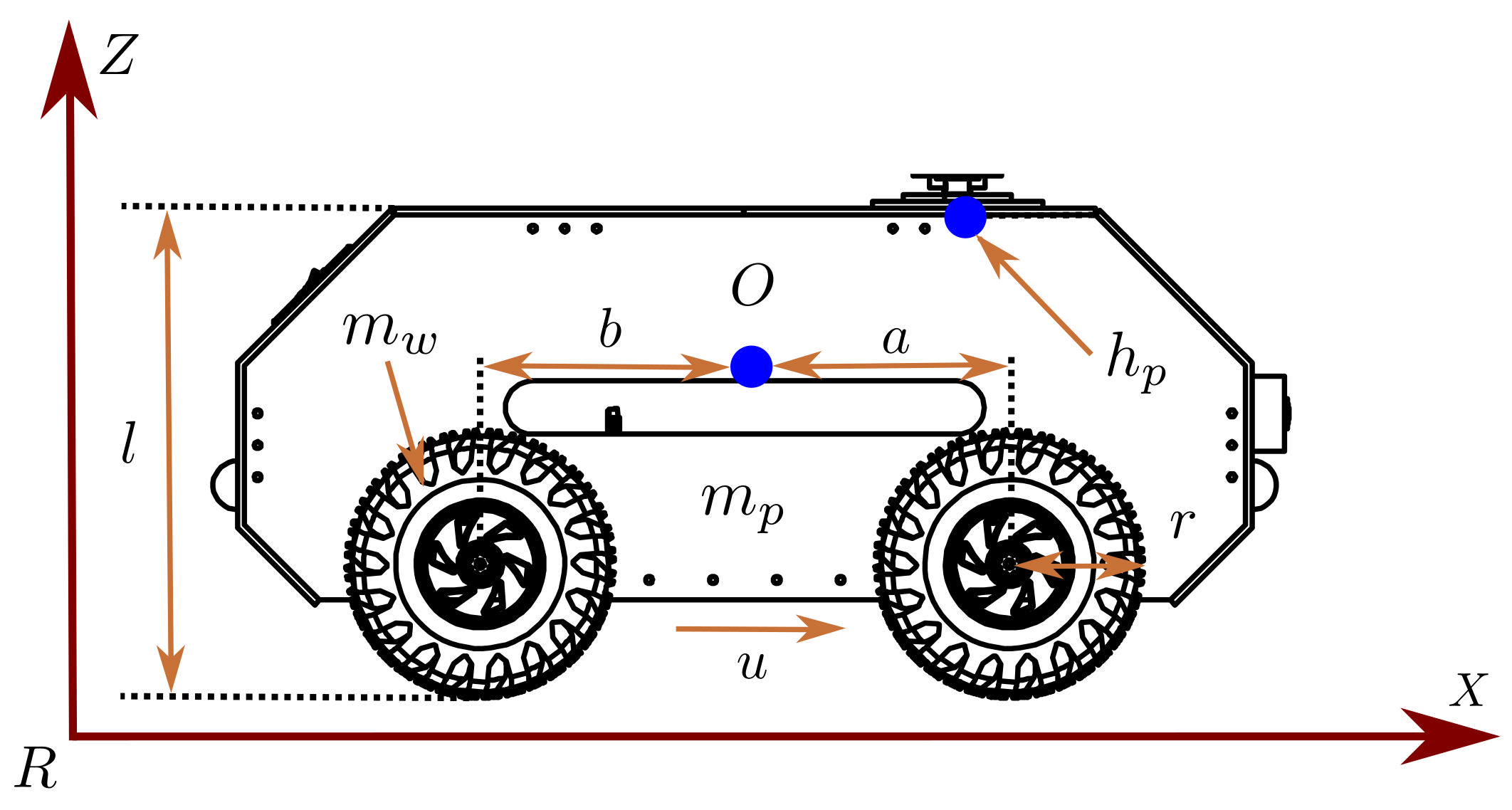
In the present work, the mobile manipulation robotic system comprises an anthropomorphic manipulator robot with three degrees of freedom linked to a four-wheel differential-drive mobile robot with three degrees of freedom, as depicted in Figure 1. This combination results in a coupled nonlinear robotic system with six degrees of freedom.
Figure 2 provides a schematic representation of the variables used to construct the mathematical model of the mobile manipulation robotic system. This representation is a projection onto the XZ-plane, which illustrates the relative positions and interactions of the components within the system, showcasing the modeling variables used. Figure 3 offers a top-down view of the coupled robotic system. This perspective allows one to comprehend the overall layout and structure of the robot. Also, it provides insights into the positioning and alignment of the system components in relation to one another, offering an understanding of the robot’s operation and motion.
Figure 4 depicts a projection of the mobile robot’s XZ-plane presenting its modeling variables. Afterwards, Table 1 provides a thorough explanation of the variables that are represented within the four figures. Each variable is carefully described, providing the necessary context to fully interpret the figures and the mathematical model.

2.2. Kinematic Modeling

The kinematic modeling of a mobile manipulation system involves the motion analysis of both the mobile robot and the attached manipulator robot. This class of robotic systems is remarkable in its ability to exhibit locomotion and manipulation skills. In this context, the establishment of two control points is defined while developing the differential kinematic modeling of the coupled robotic system, similar to the methodology presented in [68,69,70].
The control point h p describes the mobile robot’s linear and angular velocities at the geometric point where the base of the manipulator robot is located. The control point h q 3 describes the manipulator robot’s joint velocities as well as the mobile robot’s linear and angular velocities, all of it expressed at the end-effector of the coupled robotic system.
Within the considered manipulator robot’s operation framework, the differential kinematic model plays an integral role by defining the relationship between the joint velocities and the corresponding linear velocities of the end-effector. The formulation and representation of these relationships are achieved by employing the robot’s Jacobian, a pivotal mathematical concept in robotic manipulation. The central aim is to express the end-effector’s linear velocity in terms of the velocities of the manipulator robot’s joint variables. These joint variables embody the fundamental elements of the manipulator robot’s structure, each representing a unique joint’s motion parameters. The calculated linear velocity of the end effector is thus a function of these joint variables and can be expressed as
x ˙ m r y ˙ m r z ˙ m r = j m 1 1 j m 1 2 j m 1 3 j m 2 1 j m 2 2 j m 2 3 0 j m 3 2 j m 3 3 q ˙ 1 q ˙ 2 q ˙ 3
with
j m 1 1 = sin q 1 l 2 cos q 2 + l 3 cos q 2 + q 3 j m 1 2 = cos q 1 l 2 sin q 2 + l 3 sin q 2 + q 3 j m 1 3 = cos q 1 l 3 sin q 2 + q 3 j m 2 1 = cos q 1 l 2 cos q 2 + l 3 cos q 2 + q 3 j m 2 2 = sin q 1 l 2 sin q 2 + l 3 sin q 2 + q 3 j m 2 3 = sin q 1 l 3 sin q 2 + q 3 j m 3 2 = l 2 cos q 2 + l 3 cos q 2 + q 3 j m 3 3 = l 3 cos q 2 + q 3 .
It is crucial to underscore that the Jacobian illustrated in Equation (1) is fundamentally a function of the manipulator robot’s joint configuration. The specific joint configurations wherein the Jacobian exhibits rank deficiency are denoted as kinematic singularities. Such singularities limit the mobility of the manipulator’s structure, imposing a restriction on the potential directions of the end-effector’s motion irrespective of joint motions. These singularities often represent obstacles in trajectory planning that should be meticulously avoided. Furthermore, the Jacobian also establishes a relationship between the forces and torques at the end effector and the corresponding forces and torques at the joints. This relation becomes essential in manipulating the robot’s interaction with its surrounding environment, emphasizing the pivotal role of the Jacobian in the operational dynamics of manipulator robots.
With respect to the operation framework of differential-drive mobile robots, this type of system has two control variables, which are the linear and angular velocities. Through variation of these variables, this type of mobile robot can perform both linear and angular displacement in the Cartesian space. To determine the position and orientation of a differential-drive mobile robot, a rotation matrix about the Z-axis is used, taking into account the distance l p from the robot’s center of mass to the considered coupling point.
Equation (2) expresses the rotation matrix in the control point as
x ˙ y ˙ ϕ ˙ = cos ϕ l p sin ϕ sin ϕ l p cos ϕ 0 1 u ω .
In Equation (2), u and ϕ ˙ = ω , respectively, are the linear and angular control velocities of the differential-drive mobile robot, x ˙ and y ˙ are the linear velocities of the mobile robot in the Cartesian space, and ϕ is the orientation of the mobile robot around the Z-axis.
Equation (2) represents the transformation matrix from local to inertial coordinates. The numerical integration of this equation yields the position and orientation of the differential-drive mobile robot in the Cartesian space. Equation (3) defines the connection betwixt the control velocities of the mobile robot and the angular velocities of the wheels
u ω = r 2 r 2 r 2 c r 2 c ω L ω R .
In Equation (3), ω L and ω R represent the mobile robot’s angular velocities of the wheels. This equation forms the kinematic model of the differential-drive mobile robot in the local coordinate frame. This expression makes it possible to calculate the mobile robot’s control velocities based on the wheels’ angular velocities. Therefore, Equation (4) expresses the differential kinematic model of the mobile manipulation system at the h p coupling point
x ˙ y ˙ ϕ ˙ = r 2 cos ϕ + l p c sin ϕ cos ϕ l p c sin ϕ sin ϕ l p c cos ϕ sin ϕ + l p c cos ϕ 1 c 1 c ω L ω R .
Considering the earlier analysis, Equation (5) defines the differential kinematic model that describes the motion of the coupled robotic system from the mobile robot’s center of mass to the end-effector. This model incorporates the mobile robot’s linear and angular velocities as well as the manipulator robot’s joint velocities to characterize the overall motion of the system
x ˙ h 3 y ˙ h 3 z ˙ h 3 = x ˙ h p + x ˙ q 1 + x ˙ q 2 + x ˙ q 3 y ˙ h p + y ˙ q 1 + y ˙ q 2 + y ˙ q 3 z ˙ q 2 + z ˙ q 3 . .
with
x ˙ h p = cos ϕ u l p sin ϕ ϕ ˙ y ˙ h p = sin ϕ u + l p cos ϕ ϕ ˙ x ˙ q 1 = sin ϕ + q 1 ϕ ˙ + q ˙ 1 y ˙ q 1 = cos ϕ + q 1 ϕ ˙ + q ˙ 1 x ˙ q 2 = l 2 sin ϕ + q 1 cos q 2 ϕ ˙ + q ˙ 1 l 2 cos ϕ + q 1 sin q 2 q ˙ 2 y ˙ q 2 = l 2 cos ϕ + q 1 cos q 2 ϕ ˙ + q ˙ 1 l 2 sin ϕ + q 1 sin q 2 q ˙ 2 z ˙ q 2 = l 2 cos q 2 q ˙ 2 x ˙ q 3 = l 3 sin ϕ + q 1 cos q 2 + q 3 ϕ ˙ + q ˙ 1 l 3 cos ϕ + q 1 sin q 2 + q 3 q ˙ 2 + q ˙ 3 y ˙ q 3 = l 3 cos ϕ + q 1 cos q 2 + q 3 ϕ ˙ + q ˙ 1 l 3 sin ϕ + q 1 sin q 2 + q 3 q ˙ 2 + q ˙ 3 z ˙ q 3 = l 3 cos q 2 + q 3 q ˙ 2 + q ˙ 3 .
By compactly ordering and grouping like terms from Equation (5), we obtain the kinematic model of the coupled robotic system at the h q 3 control point. It is expressed in matrix form as follows
x ˙ h q 3 y ˙ h q 3 z ˙ h q 3 = cos ( ϕ ) h 3 1 2 h 3 1 3 h 3 1 4 h 3 1 5 sin ( ϕ ) h 3 2 2 h 3 2 3 h 3 2 4 h 3 2 5 0 0 0 h 3 3 4 h 3 3 5 u ϕ ˙ q ˙ 1 q ˙ 2 q ˙ 3
where the elements that compose the model of Equation (6) are
h 3 1 2 = l p sin ϕ sin ϕ + q 1 l 2 cos q 2 + l 3 cos q 2 + q 3 h 3 1 3 = sin ϕ + q 1 l 2 cos q 2 + l 3 cos q 2 + q 3 h 3 1 4 = cos ϕ + q 1 l 2 sin q 2 + l 3 sin q 2 + q 3 h 3 1 5 = cos ϕ + q 1 l 3 sin q 2 + q 3 h 3 2 2 = l p cos ϕ + cos ϕ + q 1 l 2 cos q 2 + l 3 cos q 2 + q 3 h 3 2 3 = cos ϕ + q 1 l 2 cos q 2 + l 3 cos q 2 + q 3 h 3 2 4 = sin ϕ + q 1 l 2 sin q 2 + l 3 sin q 2 + q 3 h 3 2 5 = sin ϕ + q 1 l 3 sin q 2 + q 3 h 3 3 4 = l 2 cos q 2 + l 3 cos q 2 + q 3 h 3 3 5 = l 3 cos q 2 + q 3 .
Equation (6) can also be expressed in a general form as
h ˙ = J q · v .
In Equation (7), v is the control velocity vector of the coupled system, J q is the 3 × 5 matrix from Equation (6)—also known as the Jacobian of the system—and h ˙ is the velocity vector of the end-effector in the Cartesian space. The Jacobian is crucial for motion-control purposes in the Cartesian space, as it enables the calculation of the system’s inverse differential kinematics. Due to the dimensions of the Jacobian matrix, the system exhibits kinematic redundancy.
Consequently, it is necessary to compute the pseudoinverse of the Jacobian as follows
J 1 = J T J · J T 1 .
Given Equation (8), the inverse differential kinematics of the coupled system can be expressed as
v = J 1 · h ˙ .
With Equation (9), it is possible to calculate the control velocities of the coupled system given a vector of velocities expressed in the Cartesian space.

2.3. Dynamic Modeling

Mobile manipulation robotic systems fuse the motion capabilities granted by the mobile robot with the dexterity provided by the attached manipulator robot [28]. This combination of skills imposes supplementary intricacy into the dynamic modeling procedure in contrast to modeling every robot separately. Nonetheless, to attain the elevated performance promised by a mobile manipulation robotic system, comprehensive understanding of the coordination and counterbalancing of the actions enacted by the mobile robot and the manipulator robot in a combined approach are required [69].
In this sense, the dynamic modeling of a mobile manipulation robotic system involves developing equations that describe the system’s motion under the influence of forces and torques. Therefore, the dynamic model of the mobile manipulator robot specifies these motions considering the action of the coupled system’s internal and external forces [69].
Using the Euler–Lagrange methodology yields the dynamic model of the coupled robotic system [68,69,70]. This approach is ideal for nonholonomic robots, as it enables the expression of restricted dynamics through Lagrange multipliers [71]. Furthermore, this allows for the removal of motion restrictions. As a result, the model accurately describes the dynamic evolution of the state vector q in terms of the system’s velocity vector v .
Thus, the Euler–Lagrange equations can model the nonlinear behavior of a nonholonomic mobile manipulation robotic system
d d t L q ˙ i L q i M T q λ = E · Q i i = 1 , , n .
In Equation (10), q represents the generalized coordinates of the coupled system; M q corresponds to the constraint matrix, which captures the physical limitations that impose restrictions on the system’s motion; λ contains the restraining forces exerted on the system; E serves as a full-range input transformation matrix. The components of the generalized force are denoted by Q i , where i ranges from 1 to the number of degrees of freedom denoted by n. The equation L represents the Lagrangian equation that governs the system, with
L = K P .
In Equation (11), K represents the kinetic energy, and P denotes the potential energy, where
q = x y ϕ q 1 q 2 q 3 T .
In Equation (12), q explicitly indicates the generalized coordinates of the coupled system.
The kinetic energy of the coupled robotic system is given by
K = K w L + K w R + K m P + K q 1 + K q 2 + K q 3
where the elements that compose the kinetic energy model of Equation (13) are
K w L = 1 2 m w L v w L 2 + 1 2 I y w L ϕ ˙ 2 + 1 2 I z w L ω L 2 K w R = 1 2 m w R v w R 2 + 1 2 I y w R ϕ ˙ 2 + 1 2 I z w R ω R 2 K m P = 1 2 m p v h p 2 + 1 2 I z p ϕ ˙ 2 K q 1 = 1 2 m 1 v q 1 2 + 1 2 I z 1 ϕ ˙ 2 + q ˙ 1 2 K q 2 = 1 2 m 2 v q 2 2 + 1 2 I z 2 ϕ ˙ 2 + q ˙ 1 2 + 1 2 I y 2 q ˙ 2 2 K q 3 = 1 2 m 3 v q 3 2 + 1 2 I z 2 ϕ ˙ 2 + q ˙ 1 2 + 1 2 I y 3 q ˙ 2 2 + q ˙ 3 2 .
Below are indicated the linear velocity vectors of the components of the kinetic energy model corresponding to the wheels and the chassis of the mobile robot:
v w L = x ˙ w L y ˙ w L T v w L = cos ϕ u c cos ϕ ϕ ˙ sin ϕ u c sin ϕ ϕ ˙ T v w R = x ˙ w R y ˙ w R T v w R = cos ϕ u + c cos ϕ ϕ ˙ sin ϕ u + c sin ϕ ϕ ˙ T v h p = x ˙ h p y ˙ h p T .
The correspondent linear velocity vectors of the components of the kinetic energy model corresponding to the links of the manipulator robot are also indicated:
v q 1 = x ˙ q 1 y ˙ q 1 T v q 2 = x ˙ q 2 y ˙ q 2 z ˙ q 2 T v q 3 = x ˙ q 3 y ˙ q 3 z ˙ q 3 T .
The potential energy of the coupled robotic system is given by
P = P w L + P w R + P m P + P q 1 + P q 2 + P q 3
where the elements that compose the potential energy model of Equation (14) are
P w L = 0 P q 1 = m 1 g l 1 P w R = 0 P q 2 = m 2 g l 1 + l 2 sin q 2 P m P = 0 P q 3 = m 3 g l 1 + l 2 sin q 2 + l 3 sin q 2 + q 3 .
Equations (10) and (11) describe the nonlinear and highly coupled dynamic model of the mobile manipulation robotic system through the vectorial differential equation
D q q ¨ + C q , q ˙ q ˙ + G q M T q λ = E τ τ d .
In Equation (15), D q R n × n represents the inertia matrix, which captures the system’s resistance to changes in motion; C q , q ˙ R n × n accounts for the Coriolis and centripetal forces matrix, which arises due to the system’s motion and its velocity; G q R n is the torque vector caused by gravity; τ R n corresponds to the control input vector, which encompasses the applied torques or forces to the system; and τ d R n represents the external load torque, which accounts for any additional torques acting on the system due to external factors.
Now, it is required to eliminate the restrictive term M T q λ to have a simplified expression that is much more appropriate for the tuning of motion-control strategies [69]. The model employs the matrix S q for this purpose
S q = cos ϕ l p sin ϕ 0 0 0 sin ϕ l p cos ϕ 0 0 0 0 1 0 0 0 0 0 1 0 0 0 0 0 1 0 0 0 0 0 1 .
This matrix is going to be premultiplied by the elements of the robot’s dynamic model expressed in Equation (15), as shown below
D ¯ = S T D S C ¯ = S T D S ˙ + S T C S G ¯ = S T G E ¯ = S T E .
Performing these operations yields an equation that describes the dynamics of the mobile manipulation robotic system without the motion restrictions related to the mobile robot. Elements of Equation (17) constitute the unrestricted dynamic model of the mobile manipulator robot, compactly expressed in Equation (18) as
D ¯ q v ˙ + C ¯ q , q ˙ v + G ¯ q = E ¯ τ τ d .
The dynamic representation of the mobile manipulator robot, depicted in Equation (18), is an intricate, multivariate differential equation. It exhibits continuous behavior and intensely interwoven dynamics and displays nonlinearity in its state vector [72]. Each element within this equation holds a specific meaning [73]. The term D ¯ q v ˙ signifies the inertial effect, representing changes in the system’s state of motion. The element C ¯ q , q ˙ v stands for centripetal and Coriolis forces. Centripetal forces are radial forces with a sign opposite to centrifugal forces. The Coriolis force indicates deviations in the system’s translational motion caused by its rotational components. Finally, the term G ¯ q represents the gravitational torque vector, outlining the effects of gravitational forces on the system.

3. A Motion-Control Approach for the Mobile Manipulation Robotic System

A robust motion trajectory tracking control approach for mobile manipulation robotic systems for manufacturing applications is presented in this section. The mathematical model specified in Equation (18) has found extensive application in delineating the regulated dynamics of various sophisticated nonholonomic mobile manipulation robotic systems [74,75,76]. From Equation (18), the dynamics of the planned motion trajectory tracking error e p in the controlled robotic system is then governed by
e ¨ p = w + ξ
with
w = D ¯ 1 q E ¯ τ ξ = p ¨ D ¯ 1 ( q ) C ¯ q , q ˙ v + G ¯ q + τ d .
In Equation (19), the tracking error vector between the desired and actual trajectories is defined as
e p = e p l e p a e q 1 e q 2 e q 3 = p m l p m l p m a p m a p q 1 p q 1 p q 2 p q 2 p q 3 p q 3 .
The linear and angular position reference trajectories planned for the mobile robot operation are respectively represented as p m l and p m a . Joint position reference trajectories desired for the manipulator robot operation are described as p q i , with i = 1 , 2 , 3 .
In the present paper, ξ is considered as an entirely unknown dynamic disturbance vector affecting controlled motion trajectory tracking error dynamics. Reasonable nonlinear dynamic modeling inaccuracies, parametric uncertainty, and external influences might be conveniently lumped into ξ . For design purposes of a robust control strategy, the disturbance vector ξ = ξ l ξ a ξ 1 ξ 2 ξ 3 T is locally approximated into a small, self-adjusting time window by the Taylor series polynomial expansion
ξ d 0 + d 1 t .
Parameter vectors d 0 and d 1 in the local polynomial disturbance model (22) are also unknown and are given by
d 0 = d 0 l d 0 a d 0 1 d 0 2 d 0 3 T d 1 = d 1 l d 1 a d 1 1 d 1 2 d 1 3 T .
Moreover, w is used like an auxiliary or alternatively named virtual control input vector to actively suppress uncertain polynomial disturbances. The present work exploits the integral reconstruction approach of velocity state variables introduced in [77] as well. This approach eliminates the need for velocity signal measurements and reduces the reliance on disturbed nonlinear dynamic system models. Differentiation of generalized coordinates with respect to time is avoided in this fashion, preventing the potential generation of unwanted noise during the processing of measurement signals. From Equation (19), an integral reconstructor for the velocity vector of the reference trajectory tracking error is then derived as
e ˙ ^ p = t 0 t w d t .
Notice that uncertain disturbances ξ and unknown initial conditions of the robotic system are not intentionally considered in the integral reconstructor of velocity vector e ˙ ^ p . The relationship between actual and reconstructed tracking error velocity vectors is then given as follow
e ˙ p = e ˙ ^ p + a 0 t + a 1 t 2
where the unknown parameter vectors
a 0 = a 0 l a 0 a a 0 1 a 0 2 a 0 3 T a 1 = a 1 l a 1 a a 1 1 a 1 2 a 1 3 T
depend on the initial conditions of the nonlinear mobile manipulation robotic system and polynomial disturbance model (22). Thus, unlike other approaches to active disturbance rejection control, the present contribution does not necessitate time derivatives of position output signals as well as the accurate real-time estimation of disturbances and parameters.
As a consequence, an auxiliary/virtual control input vector w is proposed as follows
w = B 4 e ˙ ^ p B 3 e p B 2 e p B 1 2 e p B 0 3 e p
with
B i = β i l 0 0 0 0 0 β i a 0 0 0 0 0 β i 1 0 0 0 0 0 β i 2 0 0 0 0 0 β i 3
where n is used to denote the n th iterated integral with respect to time, and i = 0 , 1 , , 4 . Furthermore, dynamic compensation based on integral tracking errors is included in auxiliary control to actively suppress polynomial disturbances ξ and discrepancies between actual and reconstructed velocity vectors, as outlined in Equation (24).
Taking into account the torque controllers specified in Equation (27) as
τ = E ¯ 1 D ¯ q w .
The dynamics of the closed-loop tracking error result in
e p 5 + B 4 e p 4 + B 3 e p 3 + B 2 e ¨ p + B 1 e ˙ p + B 0 e p = 0 .
Hence, stability assurance requires choosing gain matrices corresponding to the subsequent Hurwitz stable characteristic polynomials
P H ( s ) = s 5 I 3 × 3 + B H 4 s 4 + B H 3 s 3 + B H 2 s 2 + B H 1 s + B H 0 .
With this understanding, to adjust a smaller quantity of control parameters, the ensuing Hurwitz stable polynomial is taken into account for every reference position
P d i s = s 2 + 2 ζ i ω i s + ω i 2 2 ( s + P i ) .
In Equation (30), ω i ,   ζ i ,   P i > 0 are the tuning parameters. In this way, the stability assurance underpins the achievement of the desired control performance. It allows precise trajectory tracking, disturbance rejection, and error minimization, all of which are vital functions in mobile manipulation robotic systems.
Consequently, for confirming closed-loop stability and effective tracking of the planned trajectories, control gains may be chosen in the ensuing manner
β 4 i = 4 ζ i ω i + P i β 3 i = 2 ω i 2 + 4 ζ i 2 ω i 2 + 4 P i ζ i ω i β 2 i = 4 ω i 3 ζ i + 2 P i ω i 2 + 4 P i ζ i 2 ω i 2 β 1 i = 4 P i ω i 3 ζ i + ω i 4 β 0 i = P i ω i 4
As a result, this method necessitates only three tuning parameters.

4. Mobile Manipulation Robotic System Motion Control Using Artificial Neural Networks

The control strategy outlined in the robust motion control approach allows for the use of a constant control gains vector. However, it is important to note that this constant selection can be dynamically adjusted or updated as required. This adjustment or update enhances the dynamical response of the mobile manipulation robotic system. In this context, the artificial neural networks enter as intelligent entities exhibiting artificial cognition and learning capabilities. Housing a vast interconnection of neurons, often depicted as simple computational or processing units in the existing literature, the artificial neural networks serve as complex conduits for processing information [78]. From predictive data analytics to complex adaptive systems, these computational models, drawing inspiration from the neural networks found in animal brains, demonstrate exceptional efficiency as they undertake a wide range of tasks. With their innate ability to universally approximate any continuous nonlinear multivariate function, the artificial neural networks become ideal candidates for modeling and control applications across a wide range of contexts [79].
Overall, the implementation of neural networks in control systems presents a profitable feature related to the reduction of complexity and computational costs associated with certain nonlinear controllers as well as the capability for enhancing the performance of designed controllers using conventional techniques. B-Spline artificial neural networks have gained attention in recent years for their potential in control applications to straightforwardly face changing operational scenarios without the need for offline retraining of the entire network. This adaptability and the ability to handle uncertainties are particularly advantageous in complex dynamic systems, where control parameters need to be adjusted over time to maintain optimal performance, such as in mobile manipulation robotic systems.
In several interesting research articles reported in the literature, multilayer artificial networks are utilized in control design to relax the requirement of the unknown information on the mobile manipulation robotic system dynamics and external disturbances. Nevertheless, increasing the number of layers increases the number of parameters to be computed regarding the internal neuronal network outline (weighted inputs and learning rules) and the control approach (control parameters), which is significantly improved in this work by using the B-Spline artificial neural networks, allowing the alleviation of the computational efforts and easing the design and implementation process.
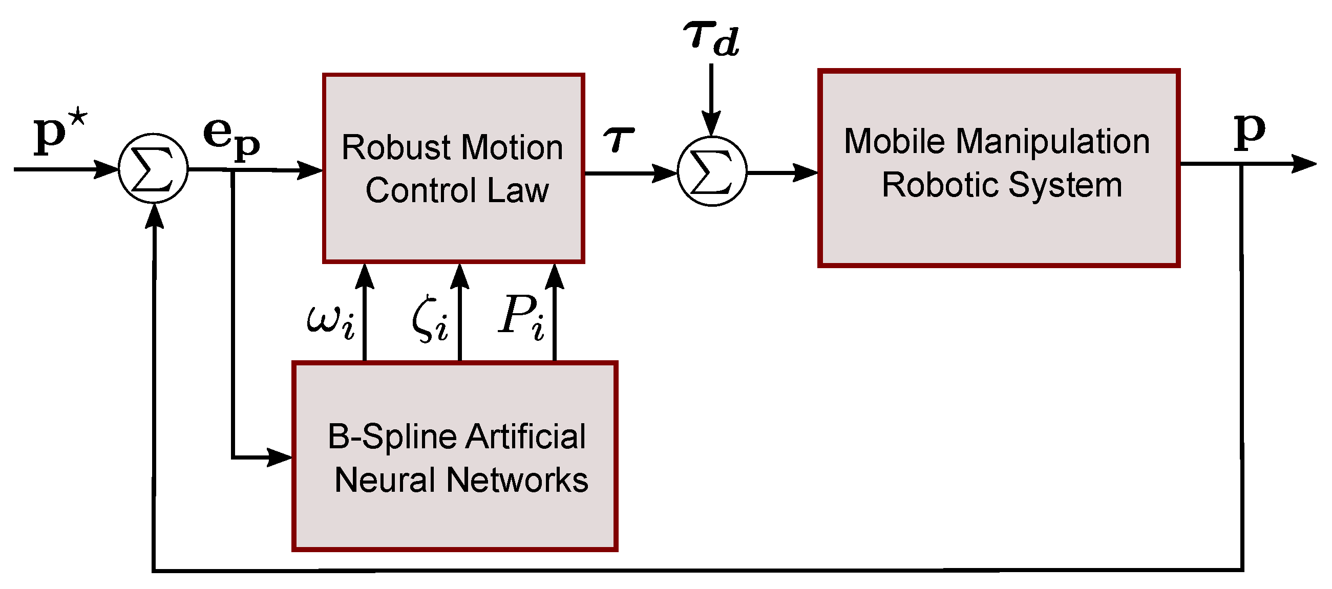
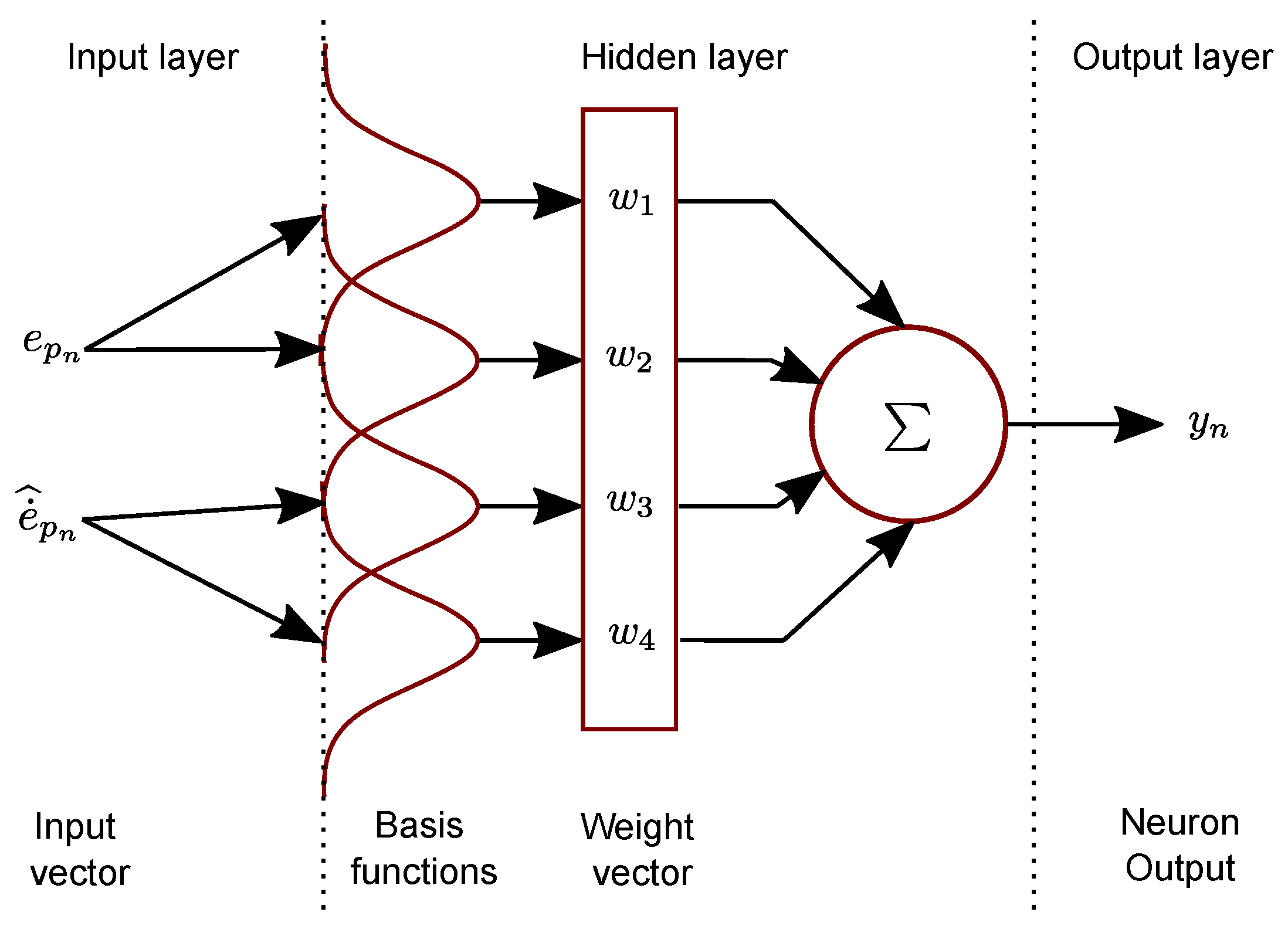
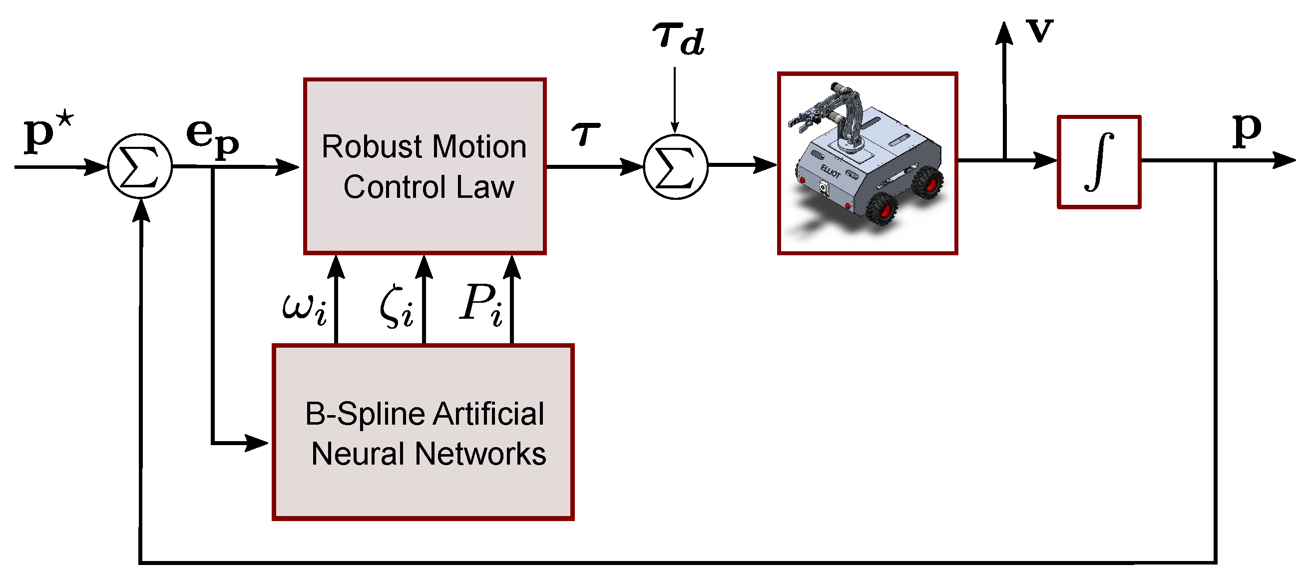
As an associative memory network, B-Spline neural networks shape the output through a weighted sum of multi-dimensional basis functions [79]. The B-Spline artificial neural network properties of real-time learning, guaranteed rate of convergence, and temporal stability [80] are suitably exploited in this work for solving the problem of determining proper values of control parameters introduced in Equation (31) within the proposed robust approach, which is graphically described in Figure 5 and Figure 6.
The control parameters have been selected to be the network output, which is dynamically updated based on the continuous learning process and the monitoring of the closed-loop tracking error, allowing adaptive system performance. Continuous training employs data information of the instantaneously desired system output for adjustment to the synaptic weights, permitting online computation of the dynamic control parameters. By performing online adjustments to the dynamic control parameters, B-Spline artificial neural networks substantially enhance the control strategy. Thus, the proposed B-Spline artificial-neural-network-based motion-control scheme is depicted in Figure 5. The illustration elucidates how the dynamic control parameters play a pivotal role in the motion-control process.
The B-Spline artificial neural networks, which build on the concept of adaptive control, harness the power of online training to offer a dynamic update pathway for the proposed control law. The adjustment structure depends primarily on the tracking error information. This feedback mechanism allows the system to adjust its behavior in response to unexpected changes in the system or environment, thus enhancing the robustness of the control strategy, as in [59,60,61,62]. A distinctive feature of the B-Spline artificial neural networks is their unique three-layer structure, which offers simplicity and reduces complexity compared to more-conventional multilayer artificial neural networks employed in identification and control applications [81]. In this sense, the B-Spline function, characterized by its boundary points, utilizes a combination of single-variable and multi-variable basis functions to generate a smooth and continuous piecewise polynomial output. This property is well-suited for system modeling and function approximation purposes [79]. Figure 6 presents the implementation of the B-Spline artificial neural networks as associative networks with adjustable synaptic weights to compute the dynamic control parameters required for the motion-tracking control scheme.
The simplified structure of B-Spline artificial neural networks makes them an attractive alternative for real-time implementations and highlights their role in augmenting the adaptability of motion-control strategies for various types of robotic systems. They demonstrate how incorporating learning-based methods can boost the development of adaptive and robust dynamic control systems. One critical advantage of adaptive control schemes is managing parametric uncertainties without needing high-gain feedback or high-frequency switching [82,83,84]. The current research aims to develop a neural motion-tracking control scheme tuned using B-Spline artificial neural networks. It is crucial to highlight that these networks adjust their synaptic weights based on varied learning indexes and inputs, thereby demonstrating an ability to manage the system’s nonlinearities and uncertainties. Perpetual learning and adaptation to the intrinsic variables of the physical system achieve this. The following output, proposed in [79], will serve as the basis for this research paper
y n = a w .
Letting
w = w 1 w 2 w j T , a = a 1 a 2 a j
where w j and a j represent the j-th synaptic weight and the j-th basis function input, respectively, and j corresponds to the number of synaptic weights. In this research, B-Spline functions are crucial for determining the approximated numerical values of the dynamic control parameters by taking the tracking error and its derivative as inputs for each neural network. The output y n defines the dynamic control parameters. The initial weight values and input thresholds can be determined through offline training of the neural network, exploring the system performance under various operating conditions using optimization algorithms [59]. The learning process heavily relies on minimizing the error between the actual output vector and the desired value. For this study, the following instantaneous learning rule is adopted [85]
w n t = w n t 1 + 𝓁 e n t a t 2 2 a t .
In Equation (33), · 2 represents the vector 2-norm or Euclidean norm, denotes the learning rate, and e n ( t ) corresponds to the instantaneous output error. This online and continuous training method updates the weight values based on the feedback of the tracking error and its derivative. This single inner-layer structure becomes a potent mechanism with the boundaries properly set by choosing the correct knot vector and basis function form. The B-Spline artificial neural networks’ functioning, different from other architectures, relies on both offline and continuously online training, which is a promising feature when properly exploited by the authors for control design of mobile manipulation robotic systems.
The weight values are updated online using a learning rule that depends on the instantaneous system output error and a learning rate value proposed after the offline training, allowing, in this fashion, proper system adaptation to different operational scenarios. On the other hand, the offline training stage, considering various sets of relationships between the outputs and inputs, is implemented for the proper selection of initial values for the synaptic weights, learning rate, and control points of the B-Spline functions. It is considered that the input is normalized, and after the offline training, it is determined that a learning rate value of 0.20 guarantees proper system functioning, allowing the manipulation system to learn to recognize and respond correctly to new operational conditions not previously faced. Additionally, Bézier polynomial trajectories are employed as the desired system outputs used for the offline B-Spline neural networks training, where several dynamic disturbances were intentionally injected for producing variations of the desired output up to 10 % , ensuring an acceptable system online response in the presence of undesired and completely unknown exogenous disturbances.

5. Numeric Simulation Results

This section presents computer simulation results to numerically demonstrate the robustness of the proposed motion-tracking control scheme for mobile manipulation robotic systems in manufacturing applications. The evaluation unfolded through four disturbed operational scenarios. The first scenario assesses the motion-control scheme’s capacity to conduct position reference tracking tasks via Bézier polynomials within the joint space of the coupled robotic system. The second scenario investigates the scheme’s aptitude for tracking position reference profiles within the joint space of the coupled robotic system even under external disturbance torques. The study showcases results from applying a nonlinear PD-like control scheme with a high dependency on some nonlinear mathematical model within this scenario. This control scheme aims to emphasize the superior performance of the proposed neural motion-tracking control strategy compared to traditional model-based controllers. The third scenario evaluates the motion-control scheme’s proficiency in tracking a motion trajectory in the operative space, a common scenario in manufacturing applications. The fourth scenario evaluates the motion-control scheme with the set of system parameters presented in [70]. However, in the presented B-Spline neural network adaptive output-feedback trajectory tracking control design for multi-input–multi-output nonlinear mobile manipulation robotic system, a wide spectrum of disturbances was considered. In all four scenarios, the performance is satisfactory, as evidenced by online updating of control gains and independence from an accurate robot dynamic model. An important aspect is that manufacturing applications demand highly precise robotic motions due to the complex and detailed procedures involved and are often subject to numerous disturbances like mechanical vibrations or sudden environmental changes. Successfully managing these disruptions is key, necessitating a control scheme that ensures precision while remaining robust against such disturbances. These experiments demonstrate effective use strategies for robotic systems in manufacturing scenarios.
During the simulations, the mobile manipulation robotic system with six degrees of freedom previously described is considered, which is characterized by the set of parameters presented in Table 2.
To eliminate abrupt motion, Equation (34) describes a position reference profile [86], which ensures smooth transitions between the initial and final positions of the robotic system
Π = Π 0 0 t < T 1 [ s ] Π 0 + Π f Π 0 B z t , T 1 , T 2 T 1 t T 2 [ s ] Π f t > T 2 [ s ] .
In Equation (34), Π 0 and Π f stand for desired initial and final values of linear and angular motion trajectories planned for the mobile manipulation robotic system. Meanwhile, B z is a Bézier polynomial defined as
B z t , T 1 , T 2 = k = 0 n δ k t T 1 T 2 T 1 k .
In Equation (35), n = 6 , and δ 1 = 252 , δ 2 = 1050 , δ 3 = 1800 , δ 4 = 1575 , δ 5 = 700 , δ 6 = 126 .

5.1. Position Reference Tracking Control in the Joint Space

Figure 7 introduces the proposed motion-control scheme for the first and second scenarios. In the first scenario, the mobile manipulation robotic system executes position reference tracking control in the mobile robot’s local coordinate frame and the manipulator robot’s joint space using the position reference profile presented in Equation (34).
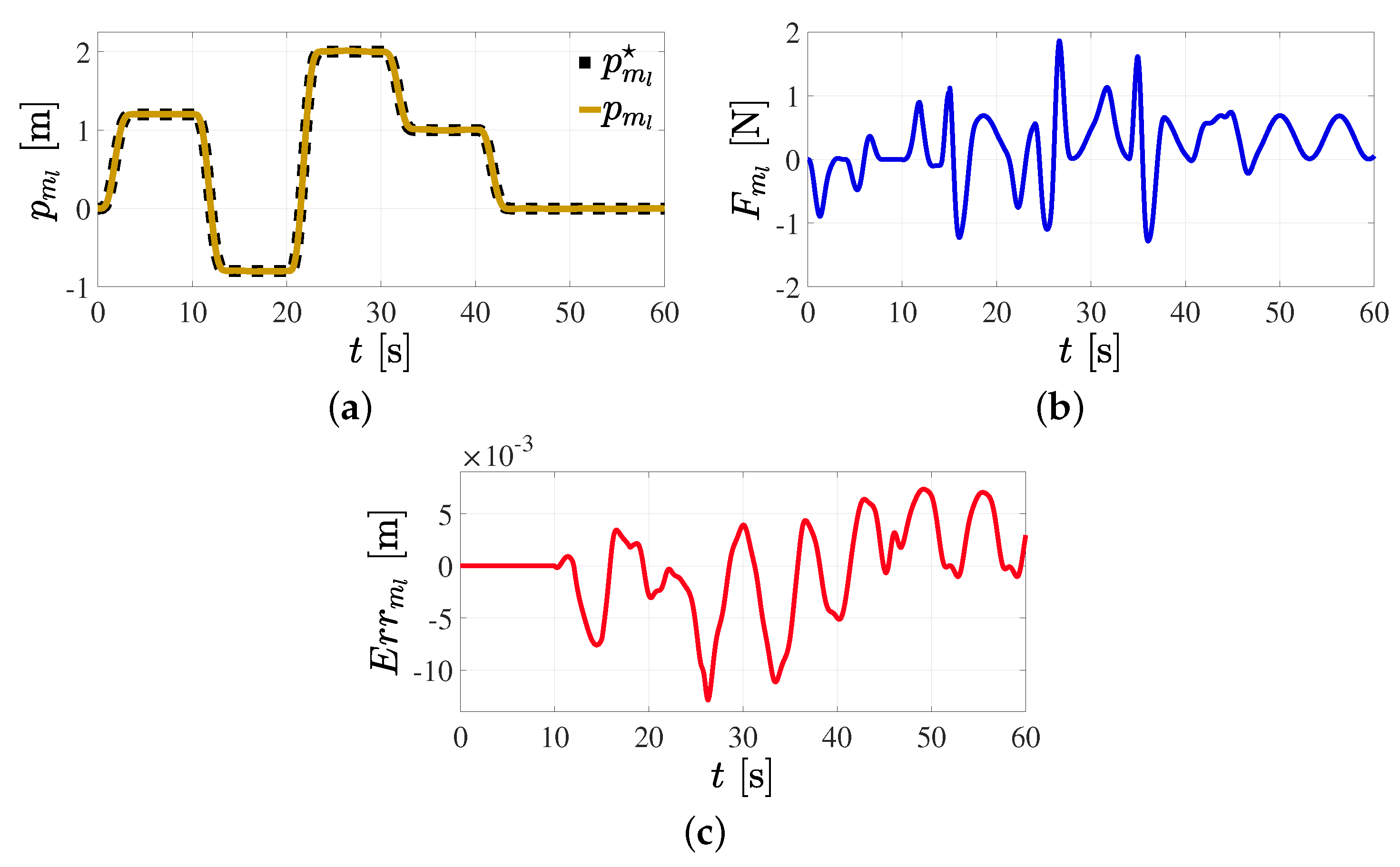
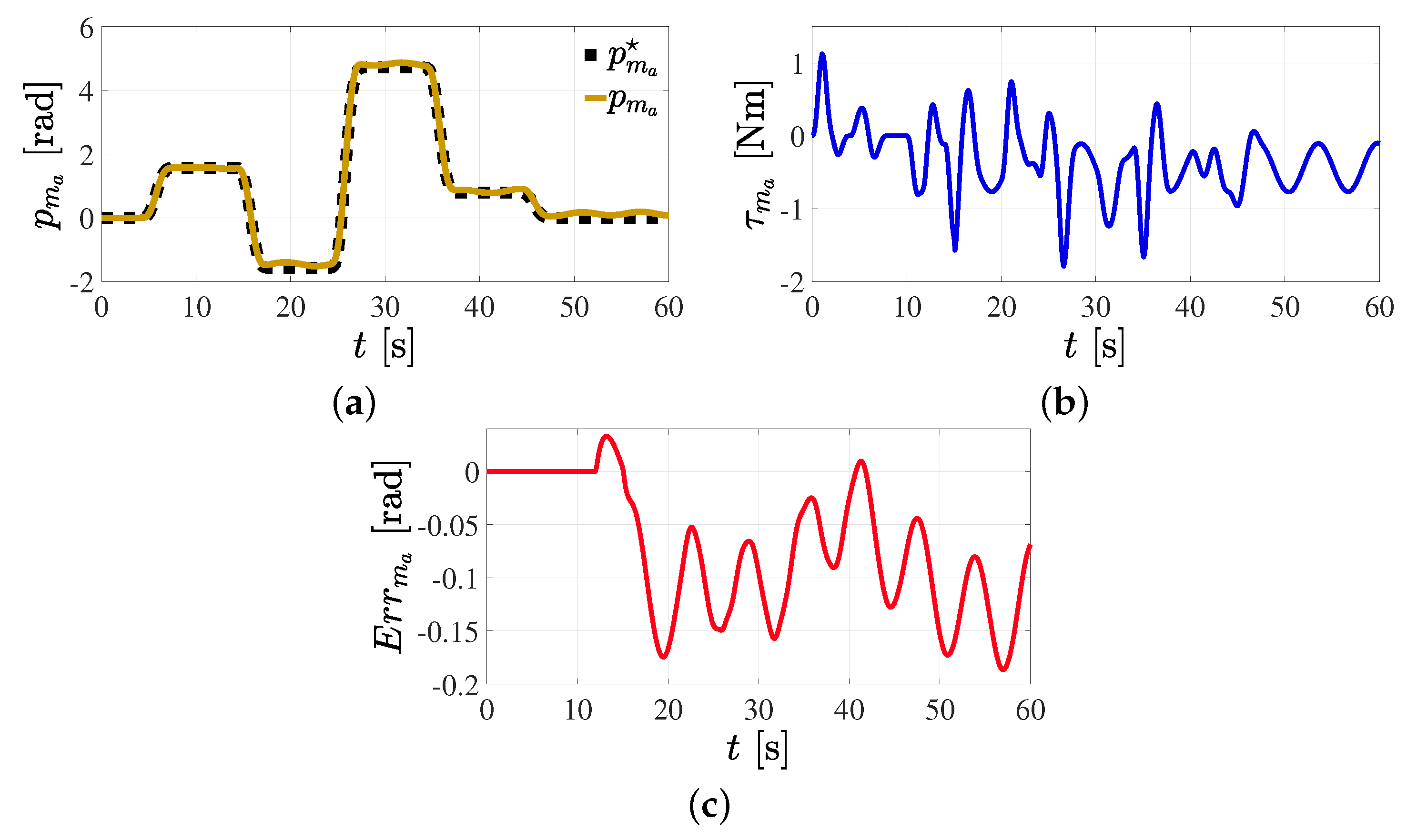
Figure 8 and Figure 9 present an insightful overview of the mobile robot’s trajectory, displaying the linear and angular position reference profiles within its local coordinate frame. These visualizations exhibit the computed driving force and torque for the intended tracking and shed light on the linear and angular position errors inherent in the mobile robot’s motions. Simultaneously, these figures depict the progressive variation to the dynamic control parameters, which is critical to accomplishing the required motion-tracking task for this scenario.
Figure 8a and Figure 9a illustrate the effective motion-tracking control exhibited in the linear and angular position profiles of the mobile robot. Figure 8b and Figure 9b further show that the demanded force and torque signals remain stable, without abrupt changes or reaching high magnitudes. Additionally, the linear and angular position error graphs, as depicted in Figure 8c and Figure 9c, provide evidence of successful tracking performance. In this context, the B-Spline neural networks prove invaluable. They provide an effective method for determining the approximate values of dynamic control parameters that align closely with an optimal initial value, thereby facilitating the execution of the desired tracking task.
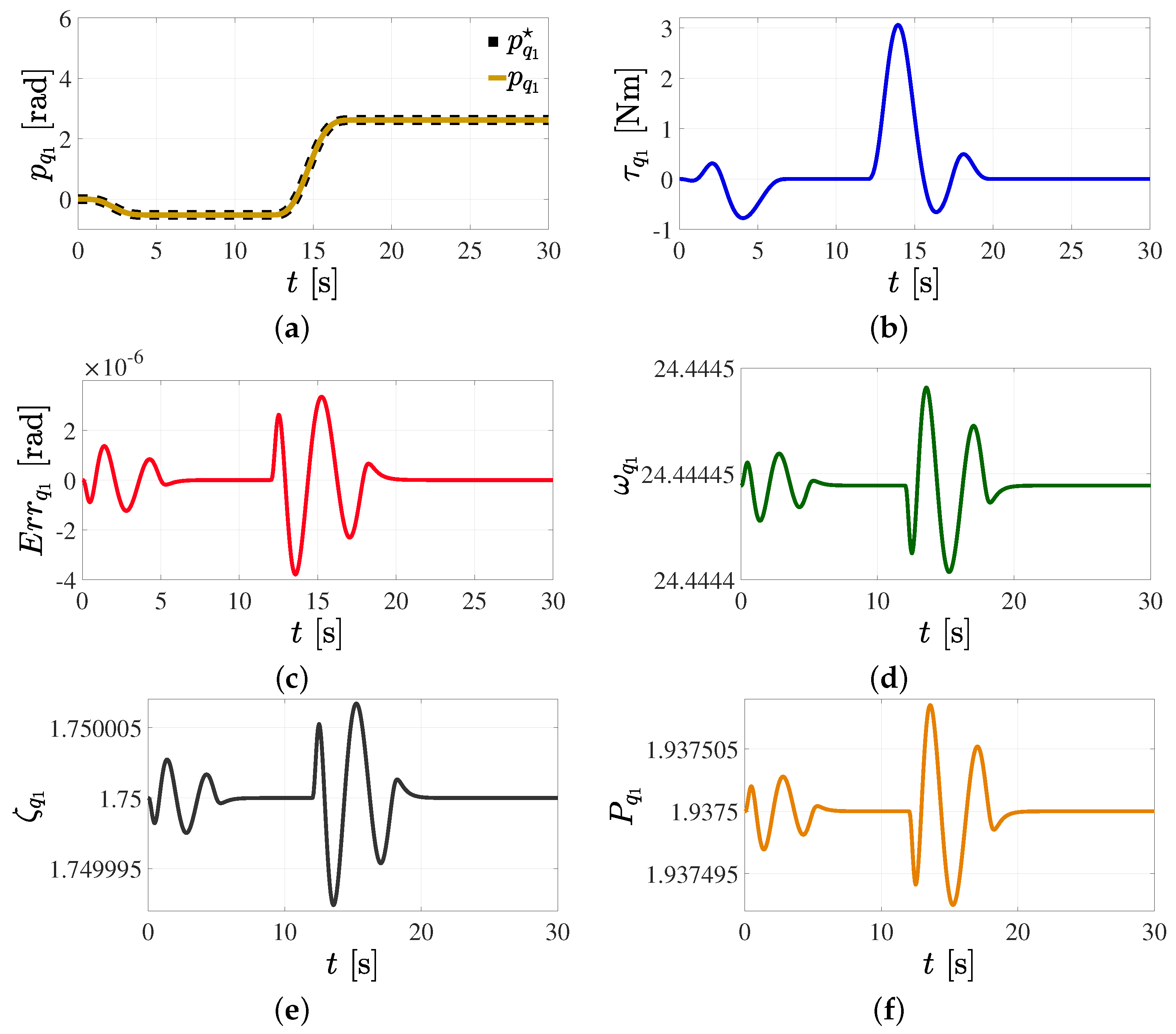
Figure 10 provides a detailed visual representation of several key aspects of the manipulator robot’s first link. Firstly, it showcases the tracking of the position reference within its joint space. Additionally, it calculates the torque signal necessary for tracking the motion profile. The figure also includes a graph of the link’s position error to illustrate the system’s performance further. Lastly, it depicts the progression of the dynamic control parameters, which are crucial for completing the motion-tracking task.
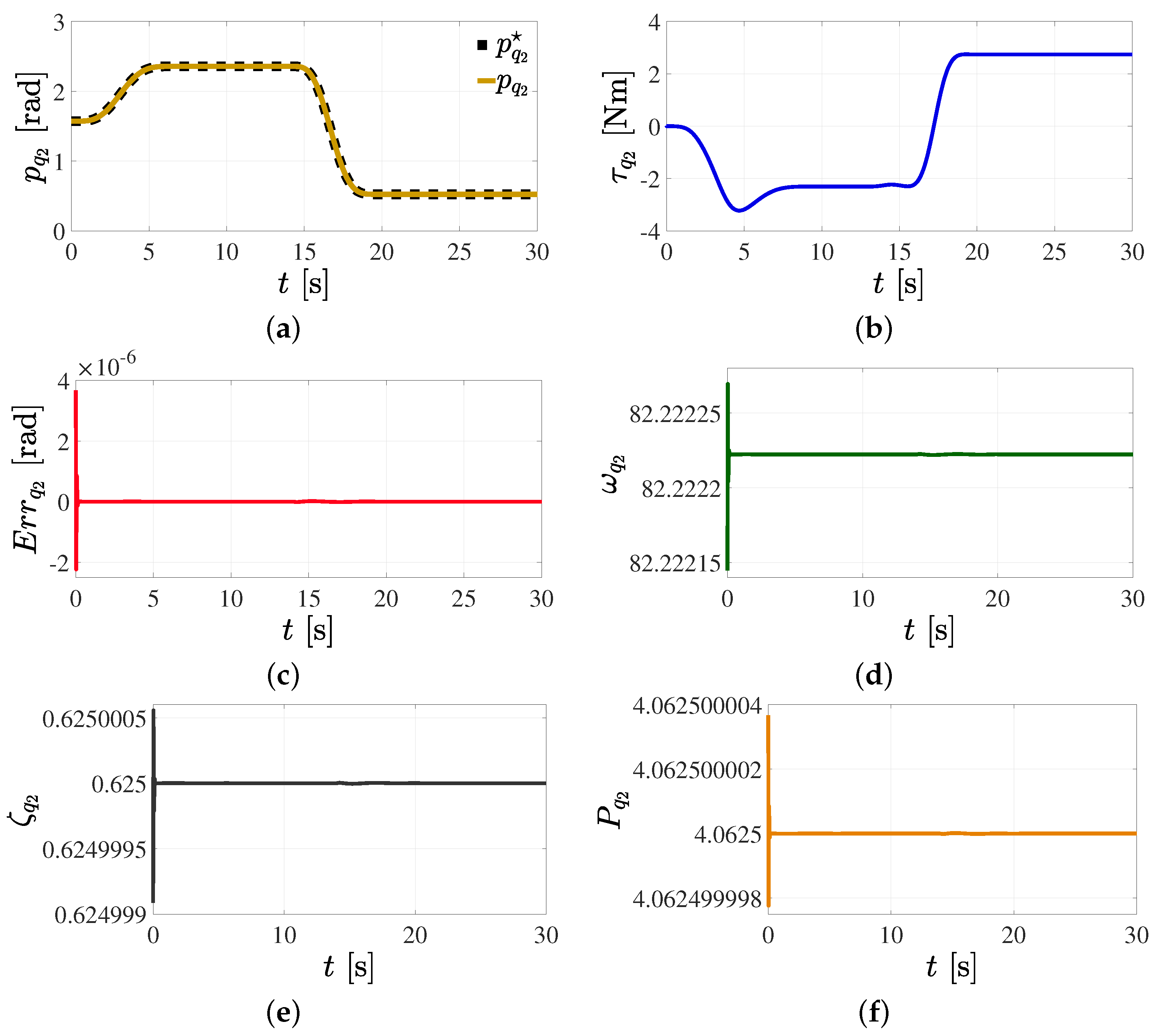
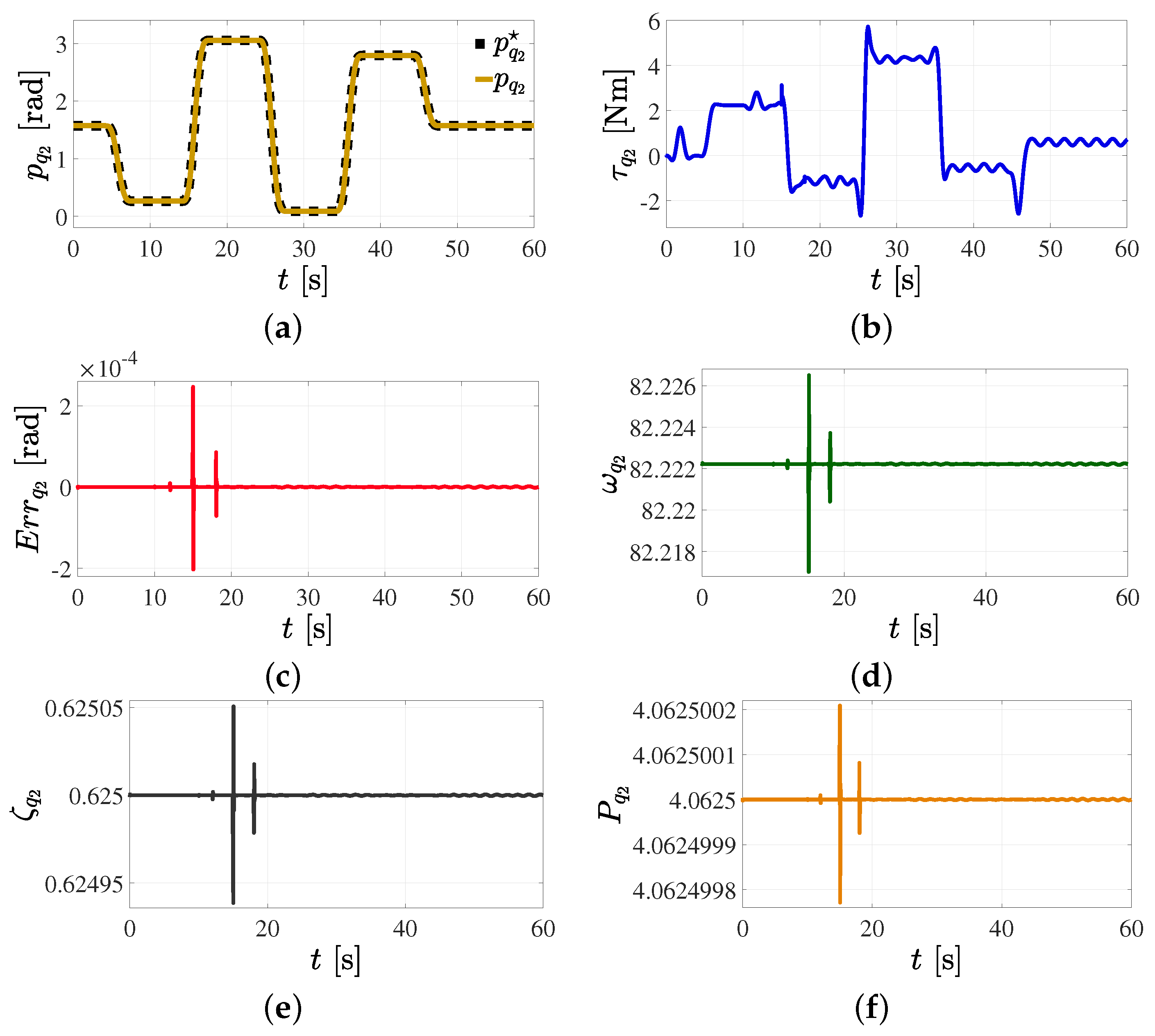
Figure 11 provides detailed insights into the operation of the second link of the manipulator robot. Figure 11a demonstrates the tracking of the desired motion reference profile within its joint space explicitly. Complementing this, Figure 11b displays the corresponding computed torque signal, a critical component for successful motion profile tracking.
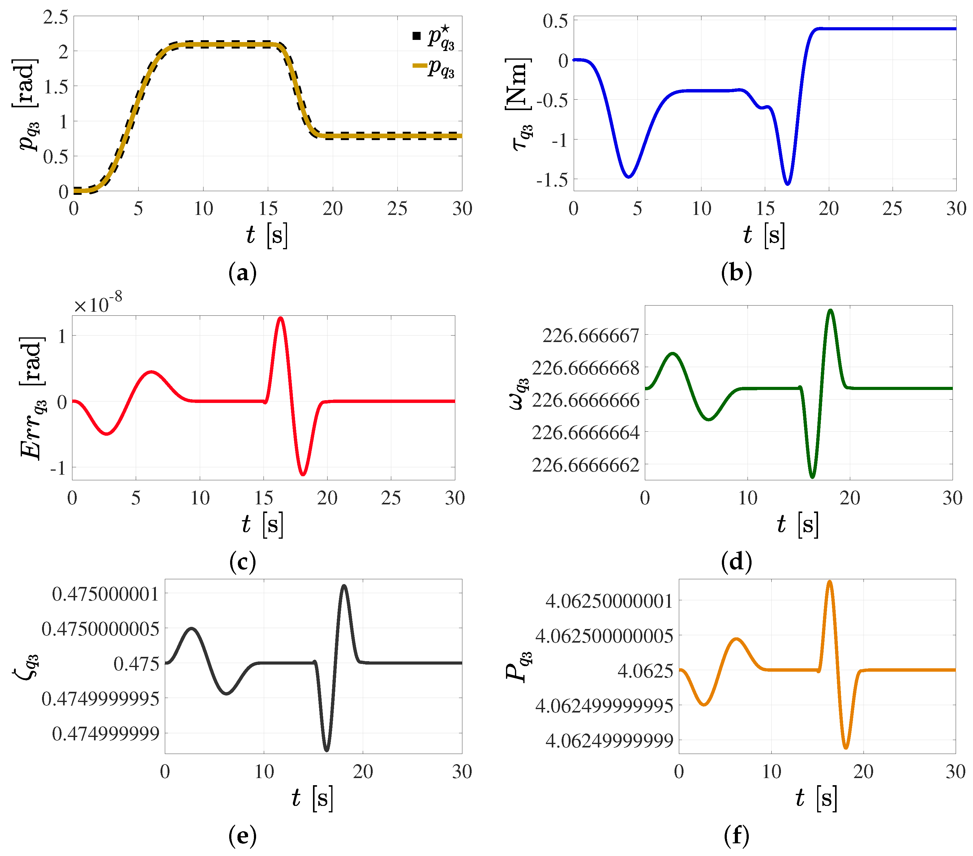
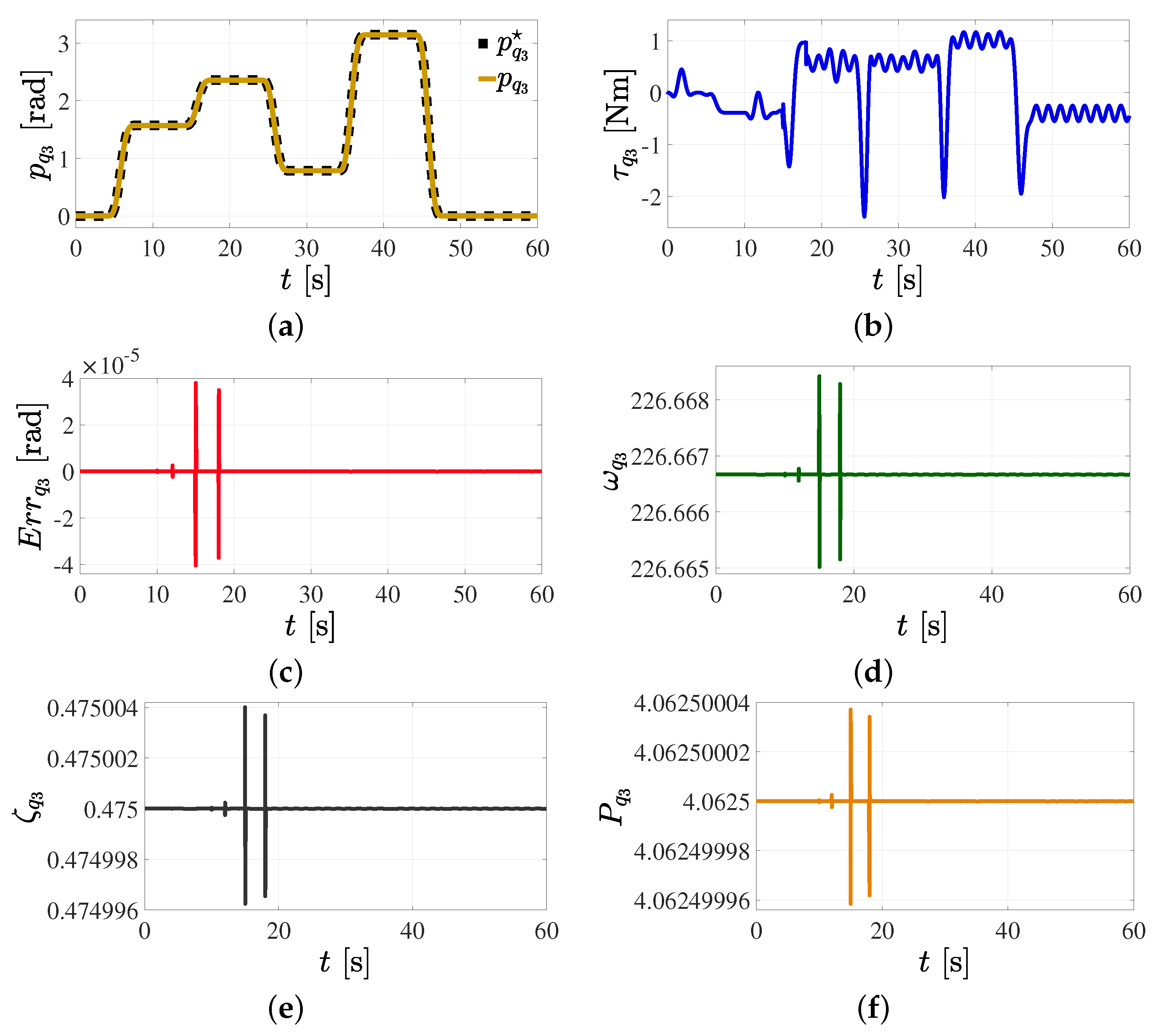
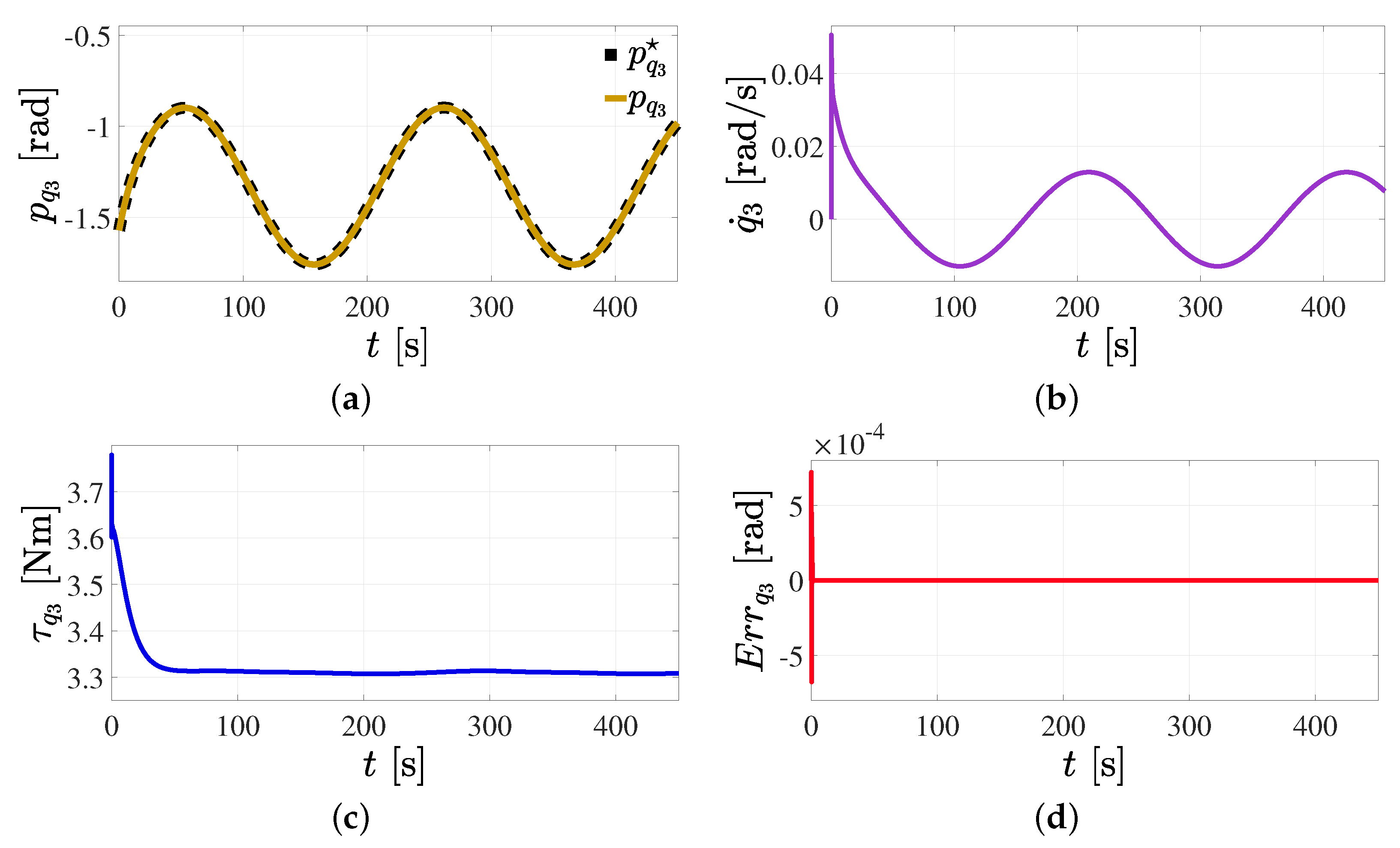
Figure 11 also presents the position error graph of the link and the evolution of the dynamic control parameters essential for the tracking task. The B-Spline artificial neural networks play a crucial role here by computing suitable numerical values for these control parameters, both in transient and steady states. As the previous figures demonstrate, this computation significantly contributes to the system’s performance. Given the system’s objective of disturbance-free motion, these control parameters exhibit minor variations from the magnitude initially calculated by the B-Spline artificial neural networks. Shifting focus, Figure 12 displays the controlled angular motion of the manipulator robot’s third link within its joint space. Along with the depiction of controlled angular motion, it exhibits the corresponding calculated torque signal necessary to accomplish the desired motion tracking of the link attached to the end-effector of the coupled system.
The results demonstrate the superior performance of the proposed control scheme in tracking the desired position reference profiles for all five variables within the mobile manipulation robotic system. Notably, the position errors reflected across these instances are of minimal magnitudes, resulting in minor variations to the control parameters. Precise regulation of these parameters, ensured by the B-Spline artificial neural networks, bolsters the efficiency and accuracy of the motion-control system. Consequently, the control scheme assures robust tracking of the desired position profiles and clearly indicates high suitability for applications requiring precision within manufacturing contexts.

5.2. Position Reference Tracking Control in the Joint Space Subjected to External Vibratory Torques

The second scenario unfolds in this subsection, showcasing the mobile manipulation robotic system’s performance as it undertakes position reference tracking control within the mobile robot’s local coordinate frame and the manipulator robot’s joint space. The position reference profile, as defined in Equation (34), provides the framework for this operation. The objective of this scenario is to demonstrate the system’s successful tracking of motion reference profiles under sudden external vibratory torques. It seeks to highlight the control scheme’s efficiency in countering these sudden disturbances during the control operation. Despite the challenging operational conditions presented, the proposed control scheme demonstrates its robustness, stability, and adaptability.
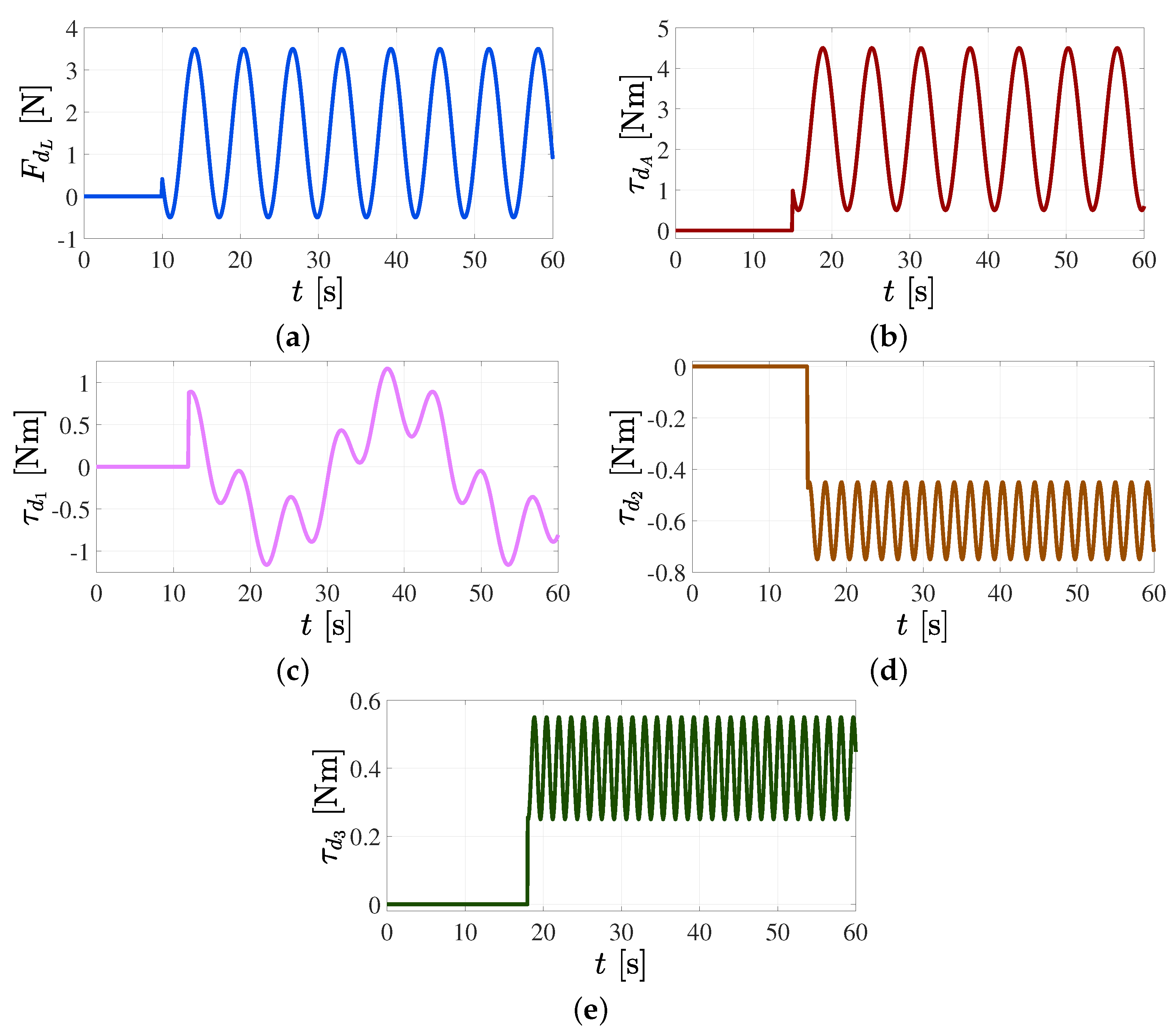
In this scenario, unknown and undesired sudden external vibratory torques deliberately disturb the mobile manipulation robotic system, as defined in Equation (36) through Equation (40). Subsequently, Figure 13 presents a graphical visualization of these perturbations. A critical aspect to observe in Figure 13 is the magnitude of the induced disturbance torques, which directly impacts the complexity of the control tasks.
Figure 13a,b showcase the disruptive force and torque proposed to disturb the mobile robot’s linear and angular motion within its local coordinate frame. Henceforth, Figure 13c–e depict the disruptive torques that aim to unsettle the articulated motion of the manipulator robot within its joint space.
F d L = 0 [ N ] 0 t < 10 [ s ] 1.5 + 2 sin ( t ) [ N ] t 10 [ s ]
τ d A = 0 [ Nm ] 0 t < 15 [ s ] 2.5 + 2 cos ( t ) [ Nm ] t 15 [ s ]
τ d 1 = 0 [ Nm ] 0 t < 10 [ s ] 0.8 sin ( 0.2 t ) + 0.4 cos ( t ) [ Nm ] t 10 [ s ]
τ d 2 = 0 [ Nm ] 0 t < 15 [ s ] 0.6 + 0.15 sin ( 3 t ) [ Nm ] t 15 [ s ]
τ d 3 = 0 [ Nm ] 0 t < 18 [ s ] 0.4 + 0.15 cos ( 4 t ) [ Nm ] t 18 [ s ]
Continuing, Figure 14 and Figure 15 illustrate the tracking of the differential-drive mobile robot’s linear and angular reference position profiles within its local coordinate frame while subjected to the external vibratory force and torque shown in Figure 13a,b. Figure 14a presents significant changes to the mobile robot’s desired linear position. Nonetheless, even in the presence of the introduced perturbation force, the robot showcases outstanding performance in adhering to the position profile. Figure 14b portrays the force necessary to uphold the tracking abilities and concurrently reject the sudden disturbance introduced during the mobile robot’s linear position tracking control.
Figure 14b illustrates that even under challenging operating conditions, the required force retains a low numerical magnitude, effectively avoiding actuator saturation. Concurrently, Figure 14c presents the mobile robot’s linear position error, which maintains a notably low magnitude, testifying to the efficacy of the motion-control scheme on this variable. The adjustments and changes to dynamic control parameters over time play a crucial role in the superior performance of the proposed control scheme. Figure 15 represents the reference tracking control of the mobile robot’s angular position within its local coordinate frame. It is remarkable that even under the sudden influence of the external vibratory torque τ d A , the tracking performance of the mobile robot’s angular position profiles demonstrates outstanding results, echoing the achievements seen previously in Figure 14a with the tracking of linear position reference profiles.
Examination of the tracking results of the mobile robot, depicted in Figure 14 and Figure 15, reveals three essential aspects. Firstly, high precision characterizes the linear and angular position reference profile tracking. Secondly, the magnitude of forces and torques emerges as a critical factor in the execution of the demanding motion-tracking task. Notably, the computed driving force and torque maintain a low numerical value despite the significant magnitude of the disturbance forces and torques. Thirdly, the linear and angular position error manifests with a remarkably small magnitude. This smallness underlines the proposed control scheme’s suitability for manufacturing tracking tasks. Applying B-Spline artificial neural networks further amplifies these findings, facilitating the system’s adaptation to a disturbed and changing environment.
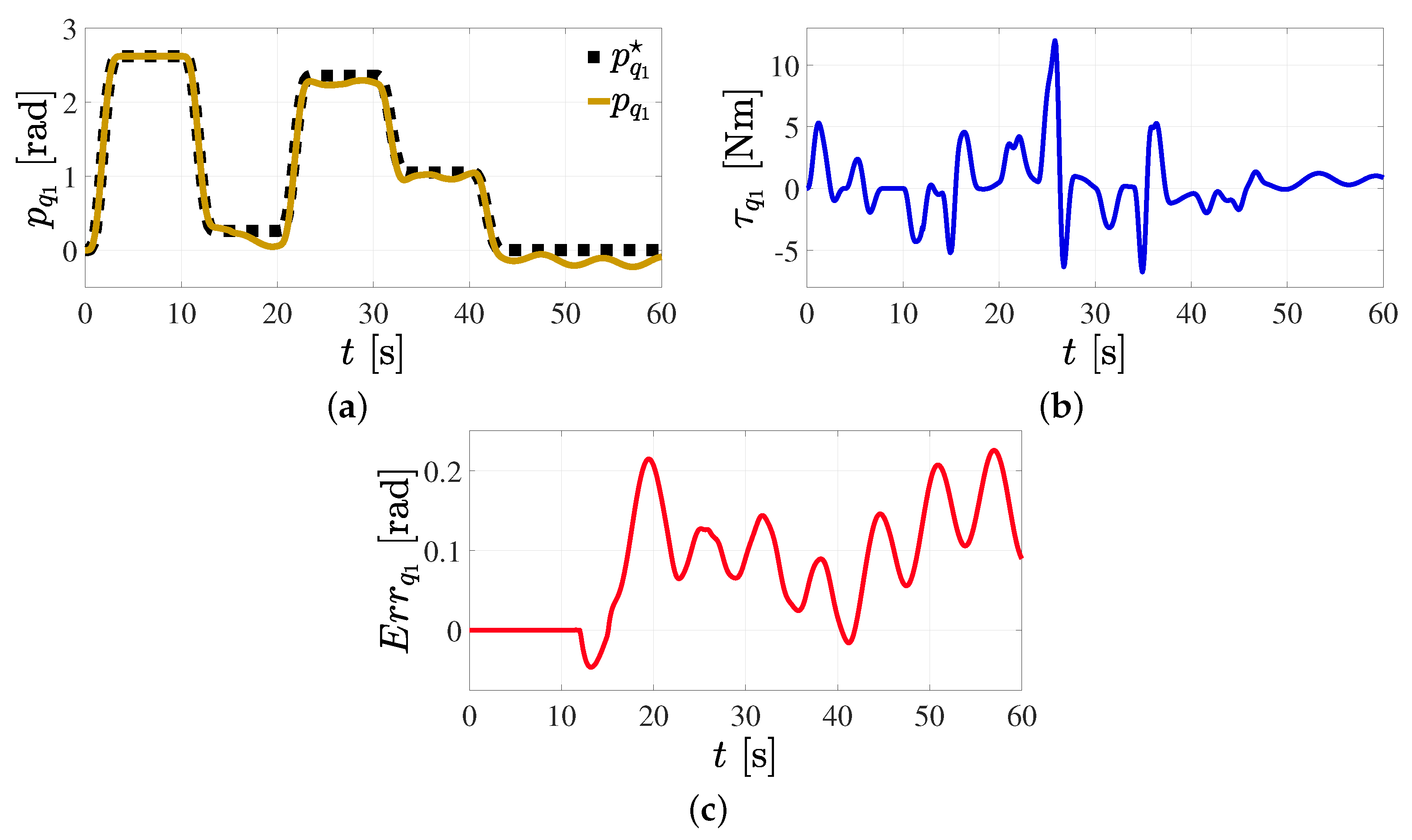
Figure 16 offers a continued exploration detailing the controlled angular motion of the manipulator robot’s first link in its joint space. The external torque τ d 1 and the computed driving torque signal for the motion profile tracking define this motion. The figure includes the position error graph of the link and the variation to the dynamic control parameters in the motion-tracking task. Several changes to the position reference profiles increase the complexity of this scenario, simulating demanding work conditions to test the system’s robustness and adaptability. Despite these challenges, the system adjusts continuously and effectively to these changes while maintaining high precision in motion tracking. This successful management of varying conditions underscores the robustness of the control scheme and, by extension, the powerful potential of the B-Spline artificial neural networks.
The numerical simulation results show remarkable adaptability and are relevant to manufacturing settings where conditions frequently change and precision is paramount. Next, as Figure 17 depicts, the external torque τ d 2 is suddenly applied to the controlled angular motion of the manipulator robot’s second link in its joint space.
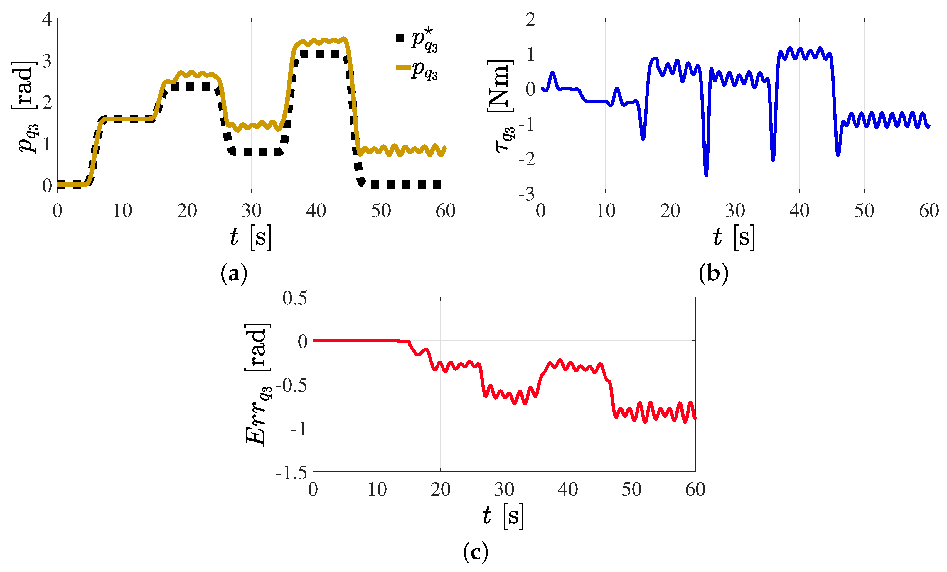
Lastly, the external torque τ d 3 influences the controlled angular motion of the manipulator robot’s third link in its joint space, as depicted in Figure 18. The precision of the manipulator robot’s three motion-tracking links within this scenario is noteworthy.
Insights drawn from the previous figures underscore the superior performance of the proposed control scheme in tracking reference position profiles in mobile manipulation robotic systems. The robotic system under consideration was subjected to challenging working conditions induced by sudden external vibratory torques and continuous changes to position profiles for tracking. While such extreme conditions are unlikely to occur in real-world environments, the demonstrated performance emphasizes the robustness and reliability of the control scheme in handling unpredictable conditions.
To compare and contrast the capabilities and the performance of the proposed neural motion-tracking control scheme, the following mathematical model-based nonlinear PD-like control policy is presented
τ = E ¯ 1 D ¯ q p ¨ K p e p K d e ˙ p + C ¯ q , q ˙ v + G ¯ q
This nonlinear PD-like control approach shows a strong dependency on detailed mathematical modeling of highly nonlinear robotic systems. This high dependence represents a possible disadvantage against inherent uncertainty in robotic system parameters and considerably disturbed operational environments. Figure 19, Figure 20, Figure 21, Figure 22 and Figure 23 depict the motion of the nonlinear PD-like control performance for reference trajectory tracking under the influences of external vibratory torques. The results show tracking errors that may be inadmissible in high-precision manufacturing applications where uncertain disturbances play a significant role.
It is important to note that the performance of the nonlinear PD-like control approach relies heavily on detailed accurate dynamic system modeling. In practical applications of robotic systems, an approximate mathematical model could not include some unmodeled dynamics and completely unknown perturbations. Parametric uncertainty may also be present in mobile manipulation robotic systems. Friction and forced vibration constitute other exogenous disturbances that could not be incorporated in some mathematical representation. Unmodeled factors might thus introduce discrepancies between the nonlinear mathematical model and the actual dynamic system, affecting the performance and reliability of the control system. Therefore, the control strategy must be robust and adaptable to account for these uncertainties and exogenous disturbances, as has been addressed in the present study.

5.3. Trajectory Tracking Control in Cartesian Space

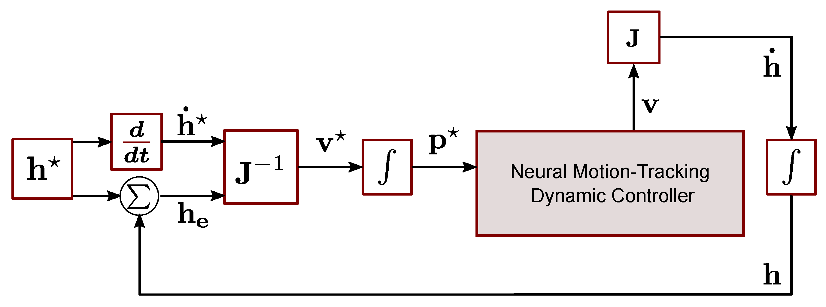
The third scenario presents the trajectory tracking control of the mobile manipulation robotic system in Cartesian space. This scenario involves precisely controlling the coupled robotic system’s position and orientation in three-dimensional space to align with a desired trajectory. The primary focus is to demonstrate the proposed controller’s efficacy in managing simultaneously the differential-drive mobile robot’s linear and angular positions and the anthropomorphic manipulator robot’s articular positions while tracking a standard manufacturing trajectory. Key goals of this research paper include ensuring high-precision tracking, robustness against disturbances, and adaptability to changing work environments. The importance of these key attributes is underlined by their critical role for successfully integrating mobile manipulation robotic systems in manufacturing applications. Providing visual reinforcement to these statements, Figure 24 illustrates the proposed motion-control scheme of the mobile manipulation robotic system operating in Cartesian space.
Inverse differential kinematics calculates tracking velocities in joint space as a function of velocities in Cartesian space of the desired trajectory for this task. The numerical integration of the joint space tracking velocities yields the joint space position reference profiles. Also, direct differential kinematics obtains the actual velocities of the robotic system in Cartesian space. Integration of these actual velocities results in the current position of the mobile manipulation robotic system. In conjunction with inverse differential kinematics, a simple kinematic-level control law generates tracking velocities in the joint space—staying within the capabilities of the robotic system’s actuators—and facilitates the transition from the initial position of the end-effector to the initial coordinate of the desired trajectory. With this methodology, the system avoids the generation of excessively high torque signals at the dynamic level.
Equation (42) expresses the kinematic control law employed in this scenario as
v = J 1 q h ˙ K p h e
where v denotes the joint space tracking velocity vector of the coupled robotic system, h ˙ symbolizes the desired Cartesian space velocity vector of the end-effector, and K p defines a proportional control gain matrix. K p has the following form
K p = k p 0 0 0 k p 0 0 0 k p .
Moreover, h e signifies the end-effector position error of the mobile manipulation robotic system in Cartesian space and is given by
h e = h x h x h y h y h z h z .
Setting the numerical values of the control gain matrix K p to 0.1 guides the robot towards the desired trajectory’s initial coordinates. Moreover, this value ensures that the calculated tracking velocities in the joint space remain within the capabilities of the robotic system.
In this scenario, a Cartesian reference trajectory is selected that is typically used in manufacturing applications. The Cartesian position references h are expressed as follows, with a simulation time of 252 s
x = 1.5 + 4.5 sin 0.025 t [ m ] y = 2.8 + 3 cos 0.025 t [ m ] z = 0.5 + 0.2 sin 0.1 t [ m ] .
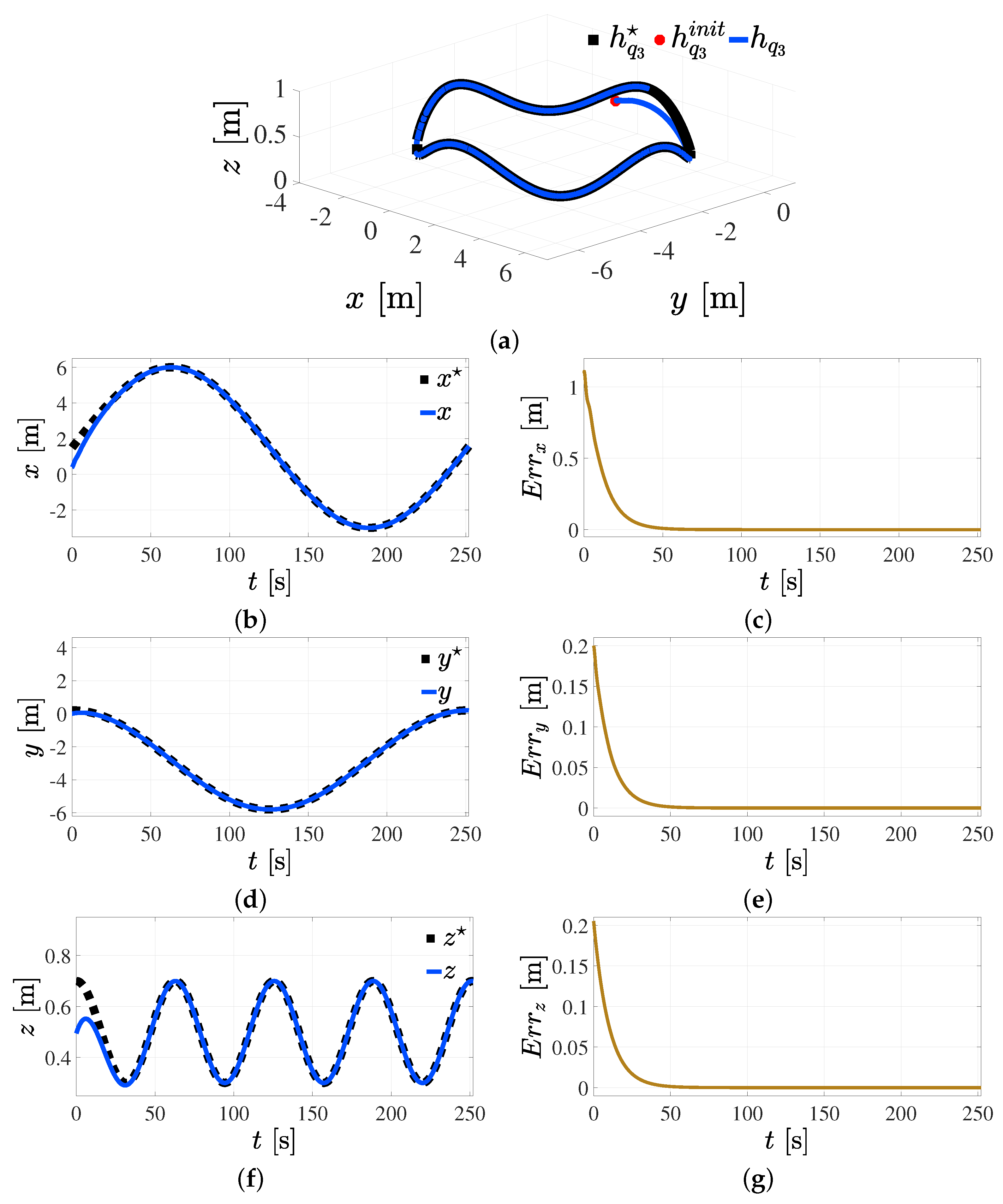
Figure 25 comprehensively depicts the trajectory tracking outcomes of the mobile manipulation robotic system operating within Cartesian space. The figure initially presents an overview of the three-dimensional trajectory tracking results, which is critical to understanding the system’s performance in a broad spatial context. It is relevant to mention that the red dot in the figure stands for the initial position of the end-effector in Cartesian space. Thus, the initial system state is intentionally located outside the desired motion trajectory planning area for purposes of control performance evaluation. The robust and efficient transference of the disturbed multi-input–multi-output nonlinear mobile manipulation robotic system from its initial state towards the planned reference trajectories is depicted in Figure 25. Following the three-dimensional overview, Figure 25 delves into a more detailed examination of trajectory tracking along each axis within the Cartesian coordinate system.
Figure 25 reveals the mobile manipulation robotic system’s performance in the Cartesian space, providing valuable insights into the robustness and the performance of the control scheme implemented for trajectory tracking tasks in a real scenario.
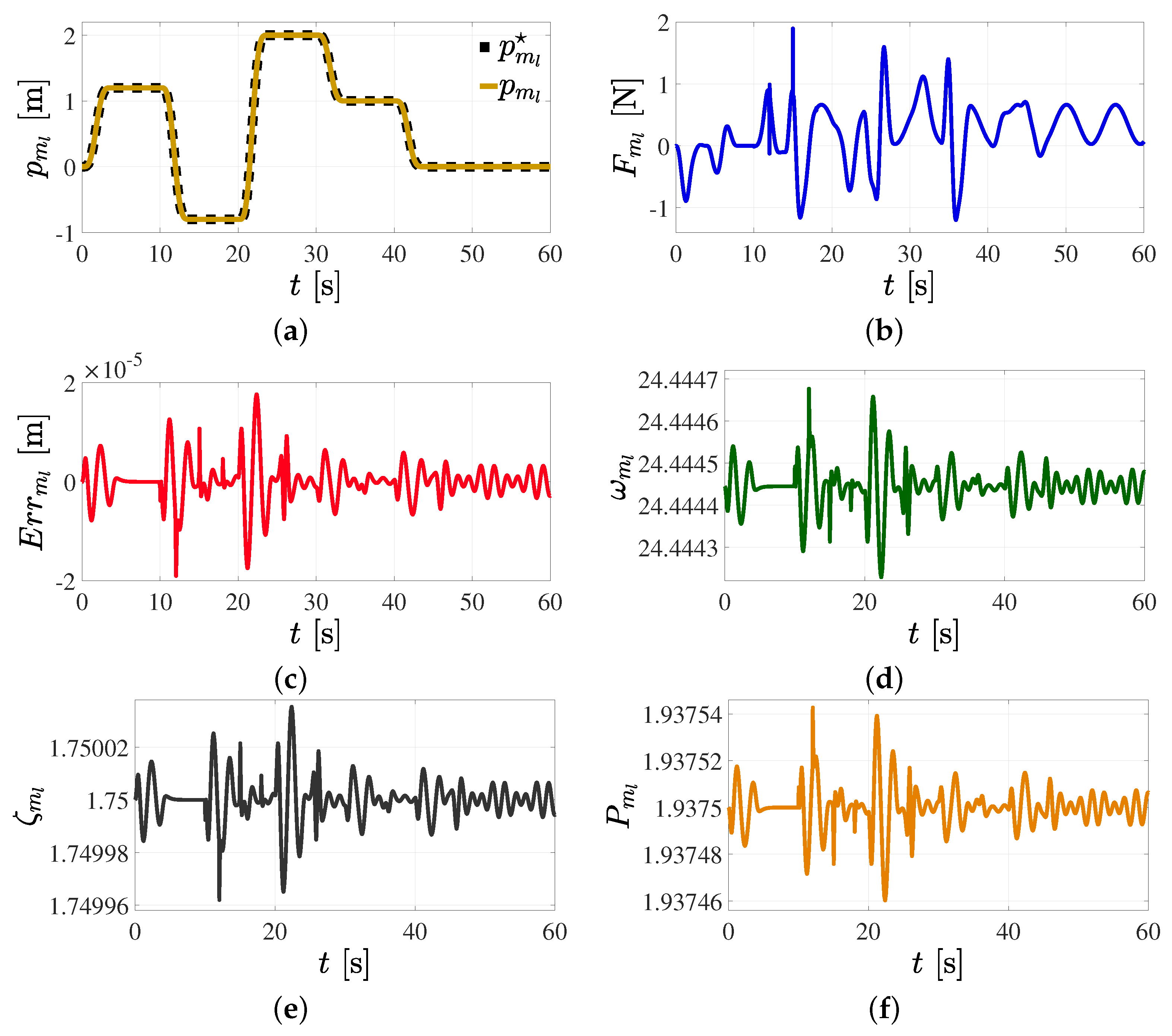
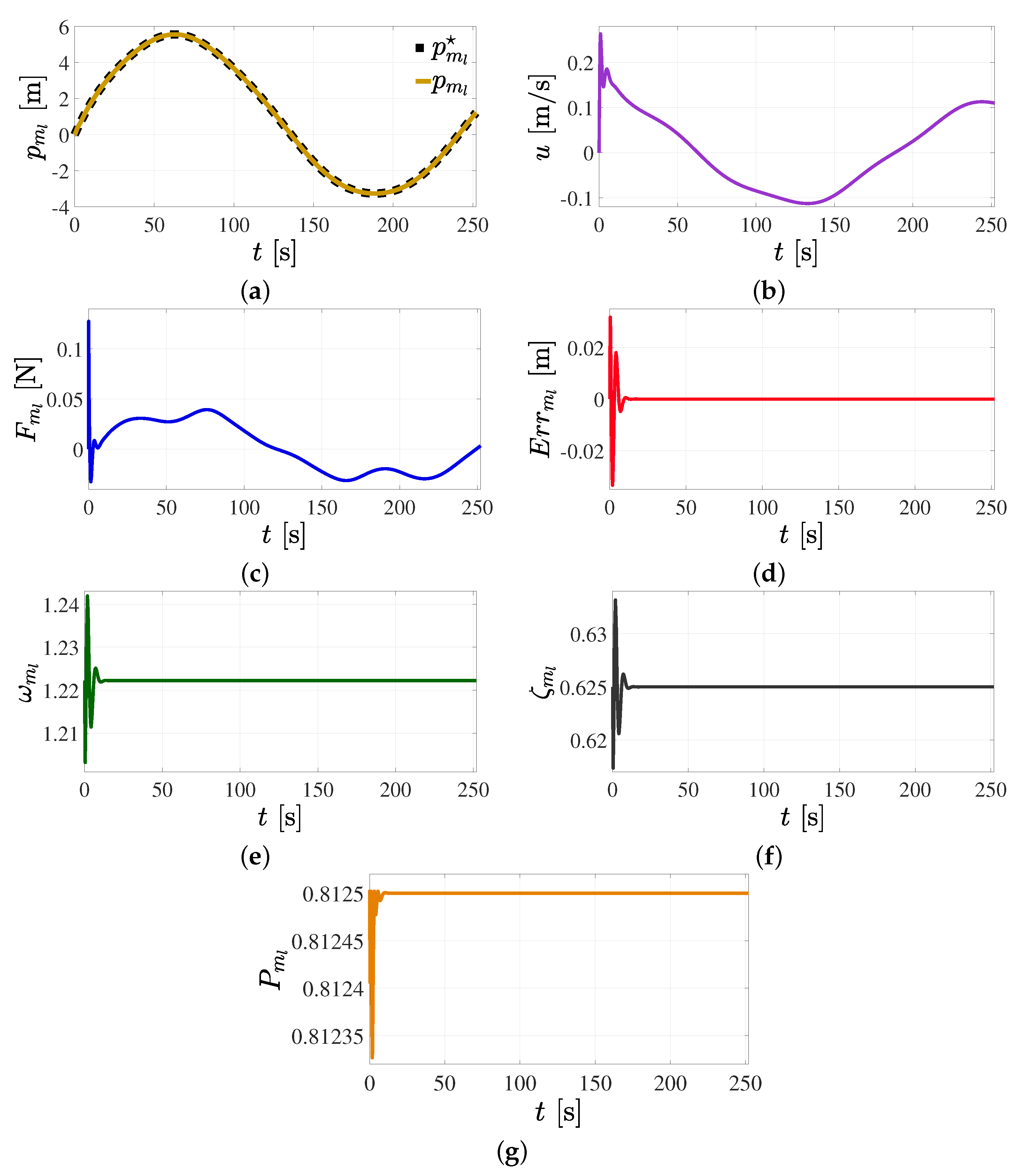
Figure 26 provides a detailed illustration of the controlled linear motion of the mobile robot within its local coordinate frame. This operation represents a crucial prerequisite for the trajectory tracking task depicted in Figure 25 to be successfully completed. Moreover, Figure 26 gives insight into the linear velocity achieved by the robotic system during the trajectory tracking task.
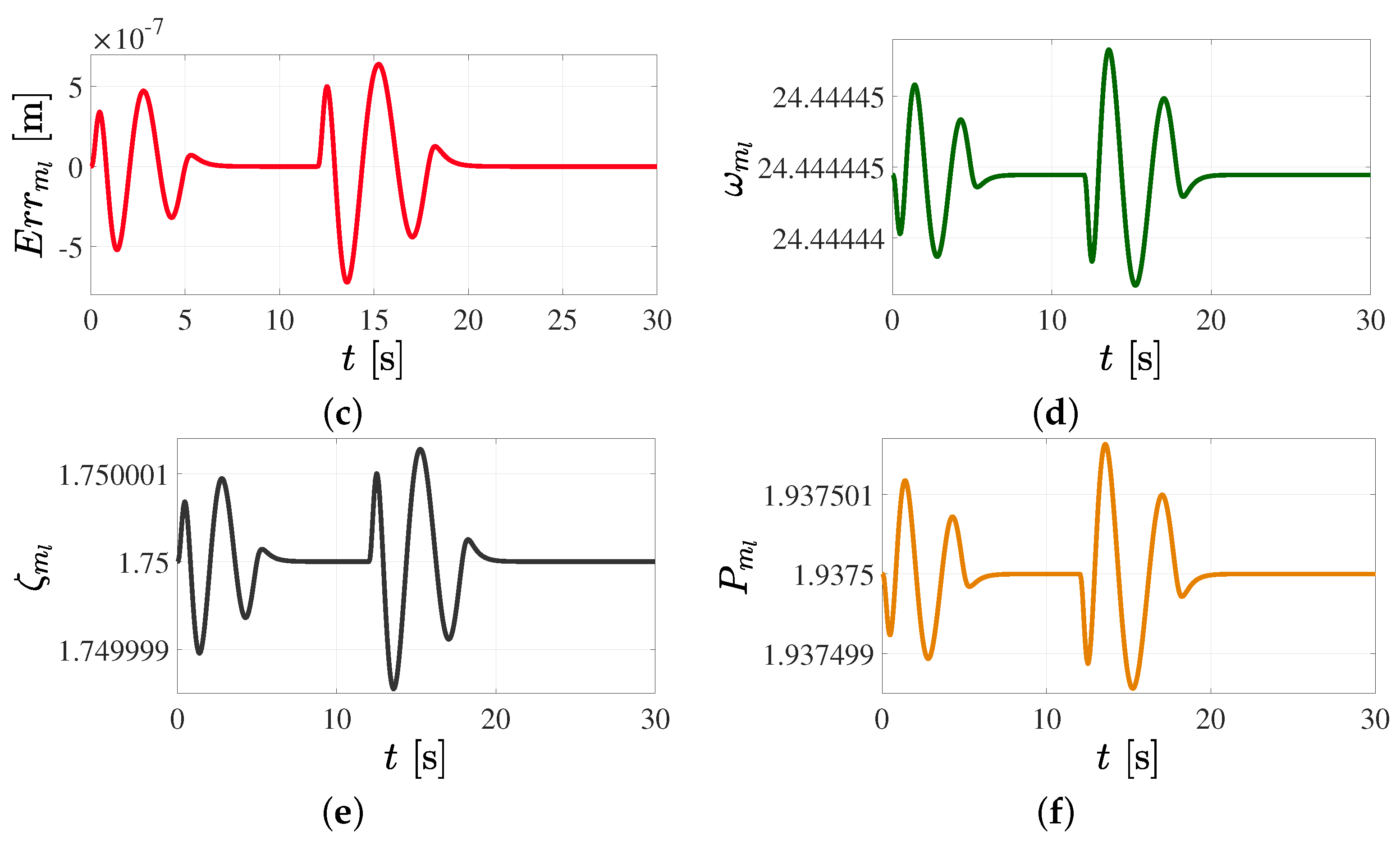
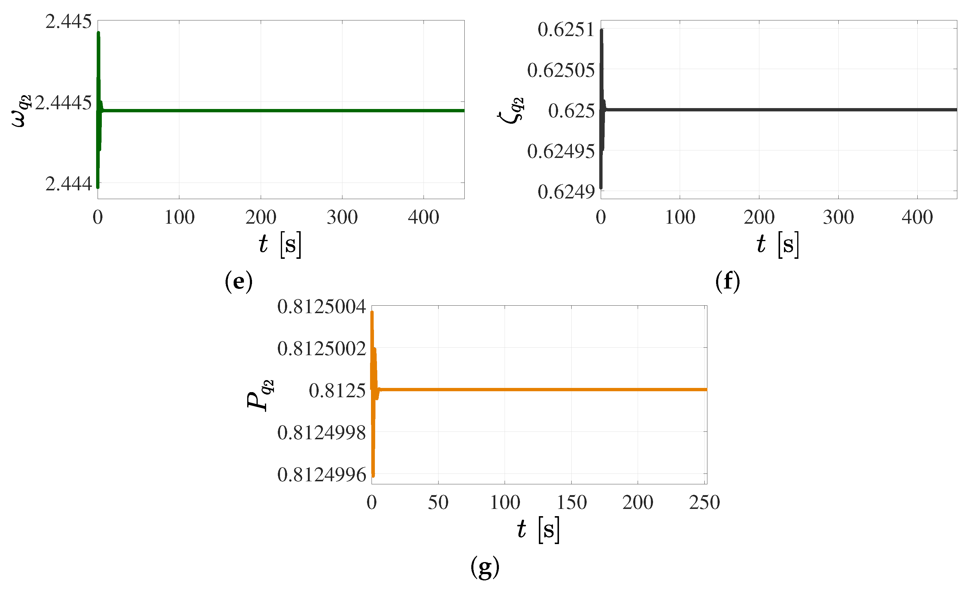
In addition to the controlled linear motion and the corresponding velocity, Figure 26 also presents a comprehensive overview of the computed driving force and the linear position error encountered during the trajectory tracking task. The dynamic control parameters—specifically ω m l , ζ m l , and P m l , which correspond to this operation—show a tendency to converge towards a constant value in a short simulation time.
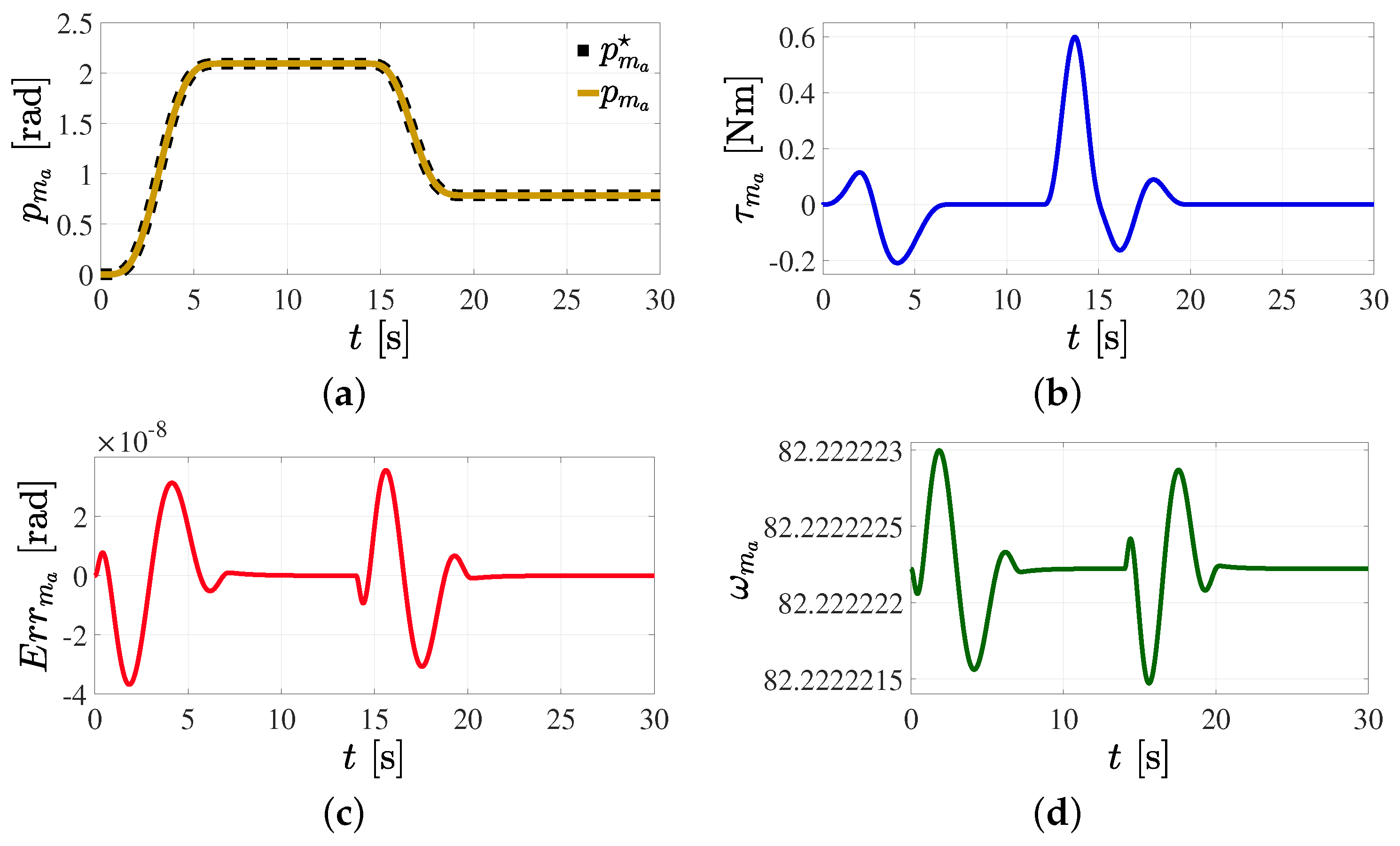
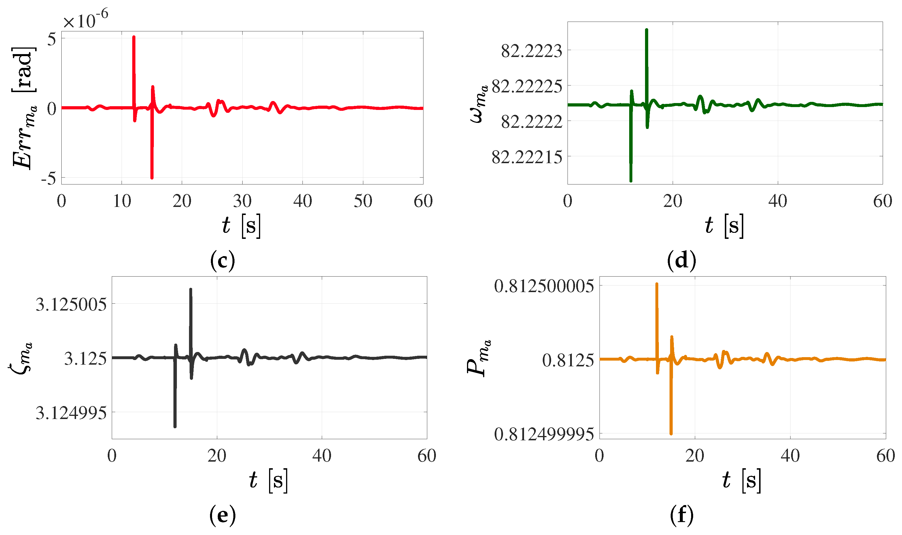
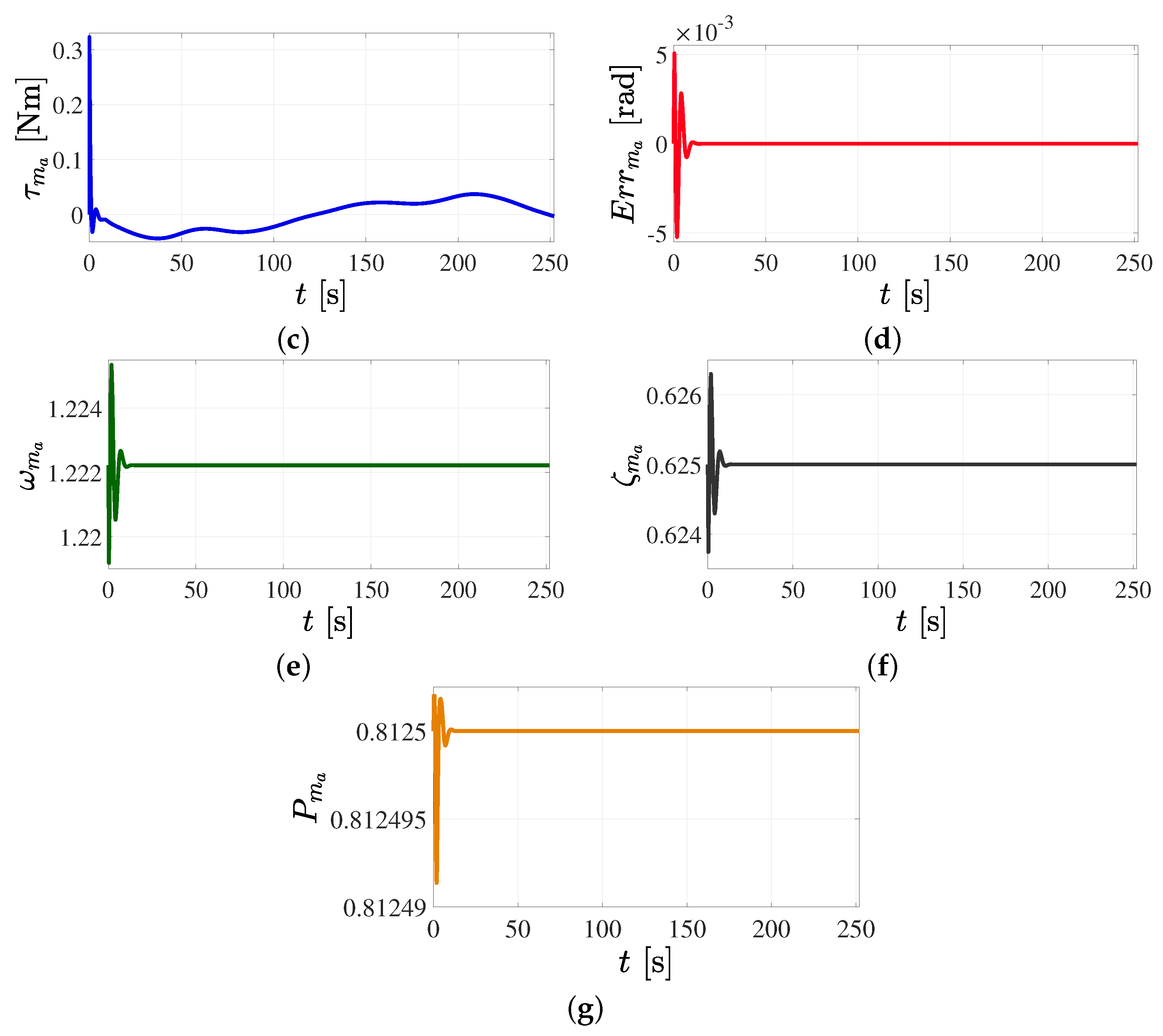
Figure 27 portrays the successful control of the mobile robot’s angular motion within its local coordinate frame, another critical prerequisite for the successful execution of the trajectory tracking task. Not only does this figure highlight the mobile robot’s ability to control its angular position, denoted as p m a , but it also showcases the magnitude of the angular velocity, ϕ ˙ , that the robot was able to attain during the required task.
The three dynamic control parameters presented in the figure showcase the adaptability and resilience of the motion-control scheme presented. These parameters, by converging to a constant value, ensure the stability of the robot’s motion, thereby significantly contributing to the successful and satisfactory completion of the trajectory tracking task.
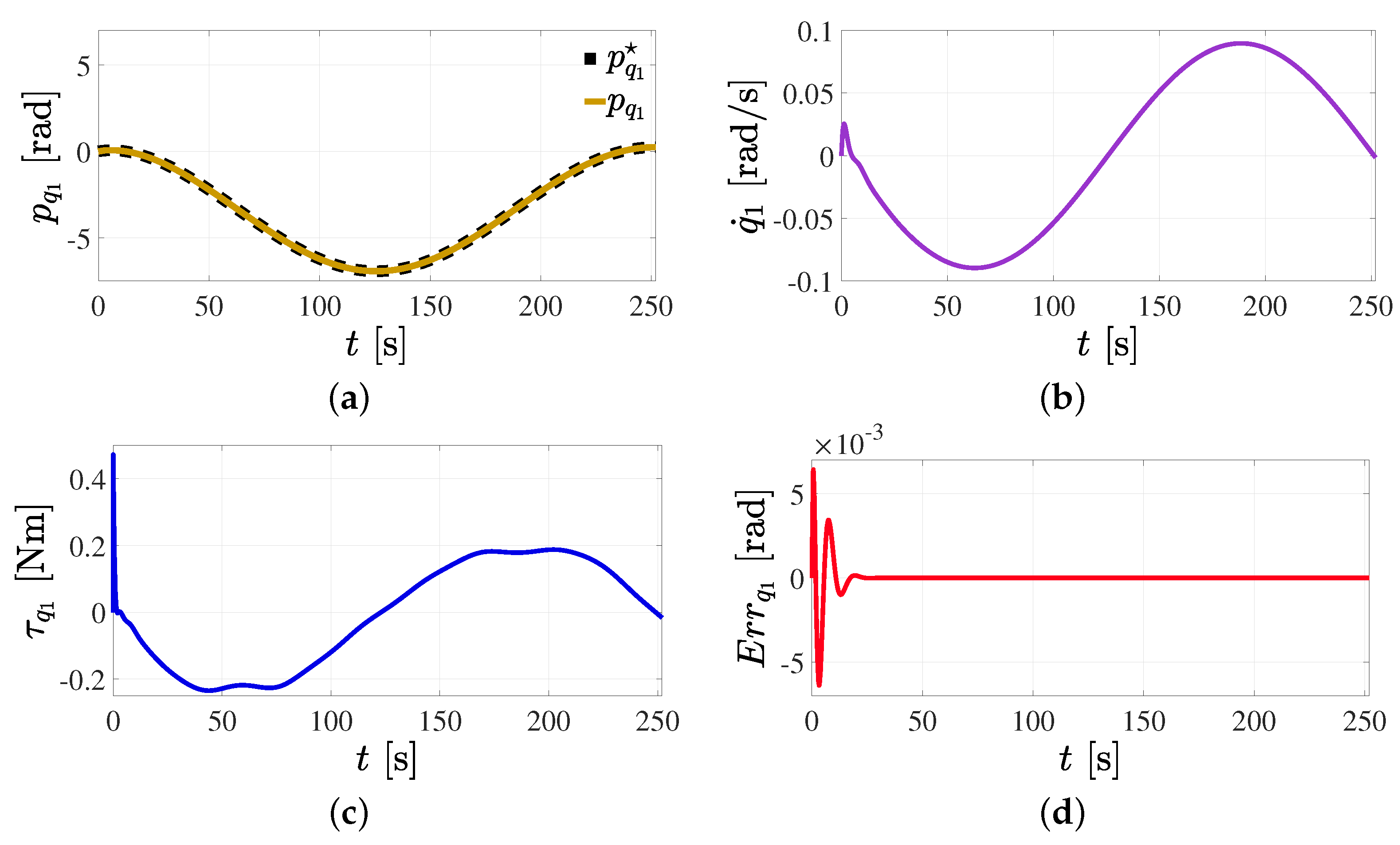
Figure 28 illustrates the controlled angular motion of the manipulator robot’s first link within its joint space, which is a pivotal requirement for successfully completing the trajectory tracking task depicted in Figure 25. This figure also displays the angular velocity achieved during the trajectory tracking task.
Further examination of Figure 28 reveals the computed driving torque and the angular position error encountered during the trajectory tracking task. Torque is an essential factor in the performance of angular motions, especially in this link. This stems from the fact that it carries the total load of the manipulator robot; thus, it is anticipated that this link necessitates a higher degree of torque to execute the needed motions.
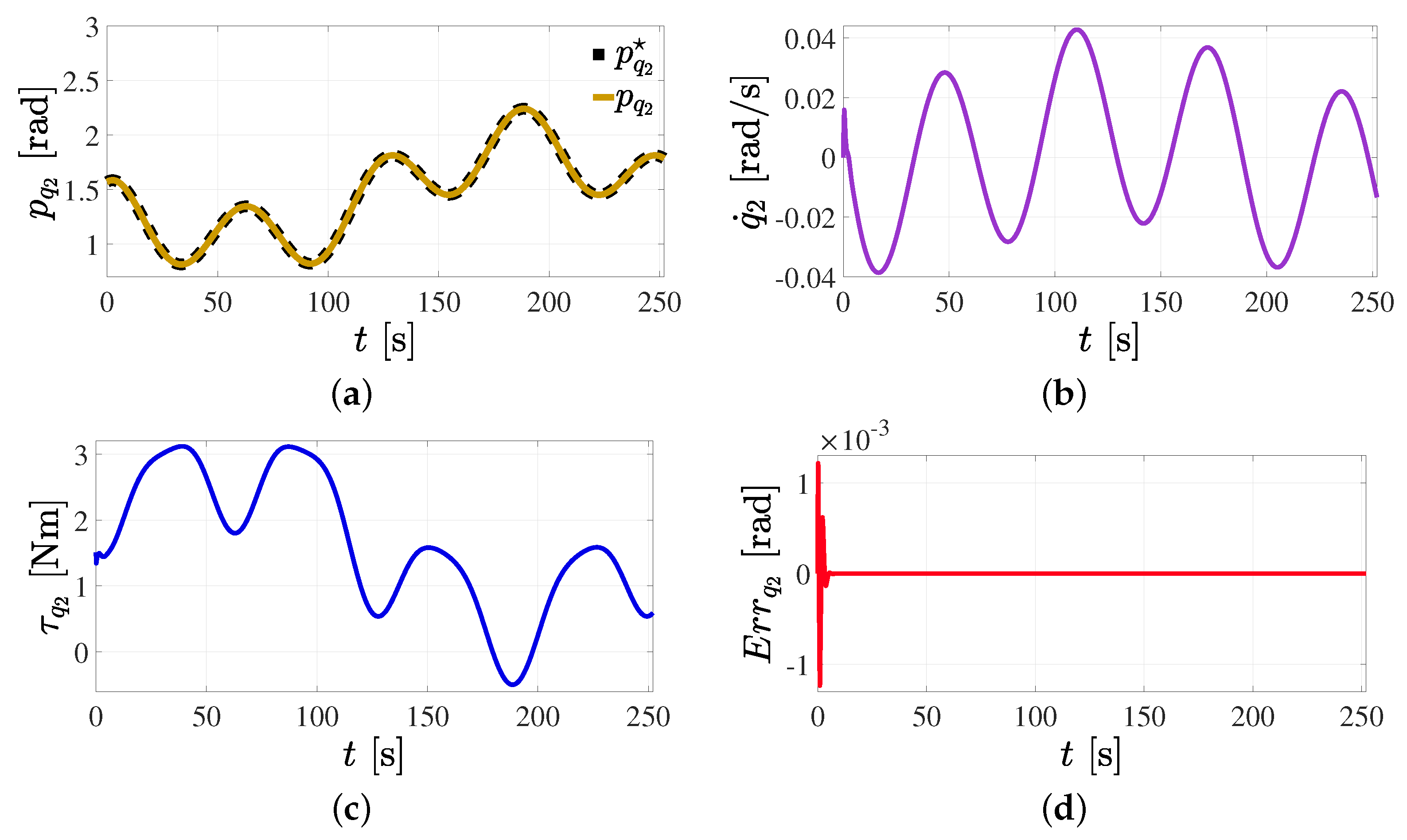
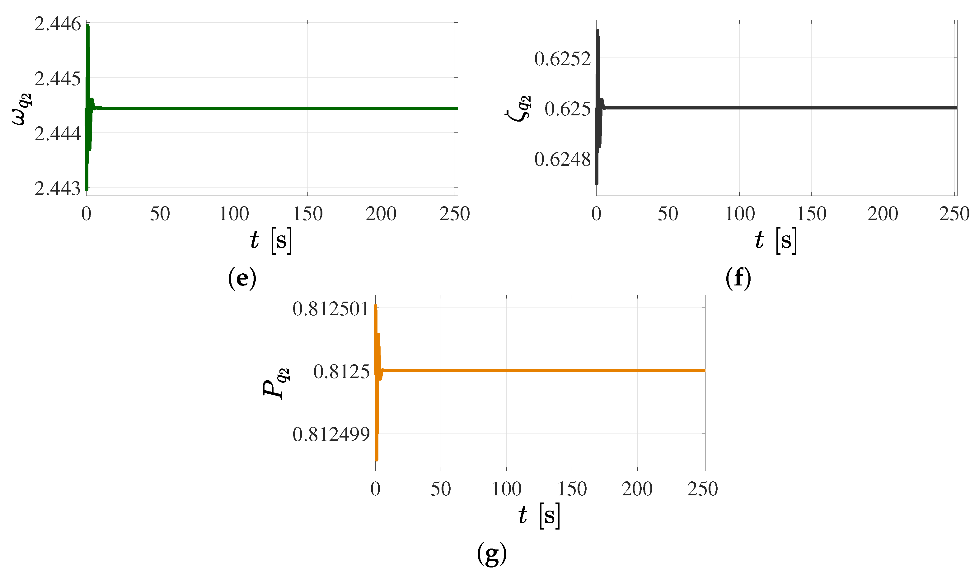
Figure 29 illustrates the controlled angular motion of the manipulator robot’s second link. The control of this motion within the joint space is another one of the fundamental requirements for successfully completing the trajectory tracking task, as previously depicted in Figure 25. This figure also displays the angular velocity achieved during the trajectory tracking task.
The figure points to the dynamic control parameters corresponding to this variable. These parameters converge to a constant value, highlighting the adaptability of the control scheme. The convergence to steady state is instrumental for enabling the task’s satisfactory completion. This pattern also signifies the stability of the control scheme in the task.
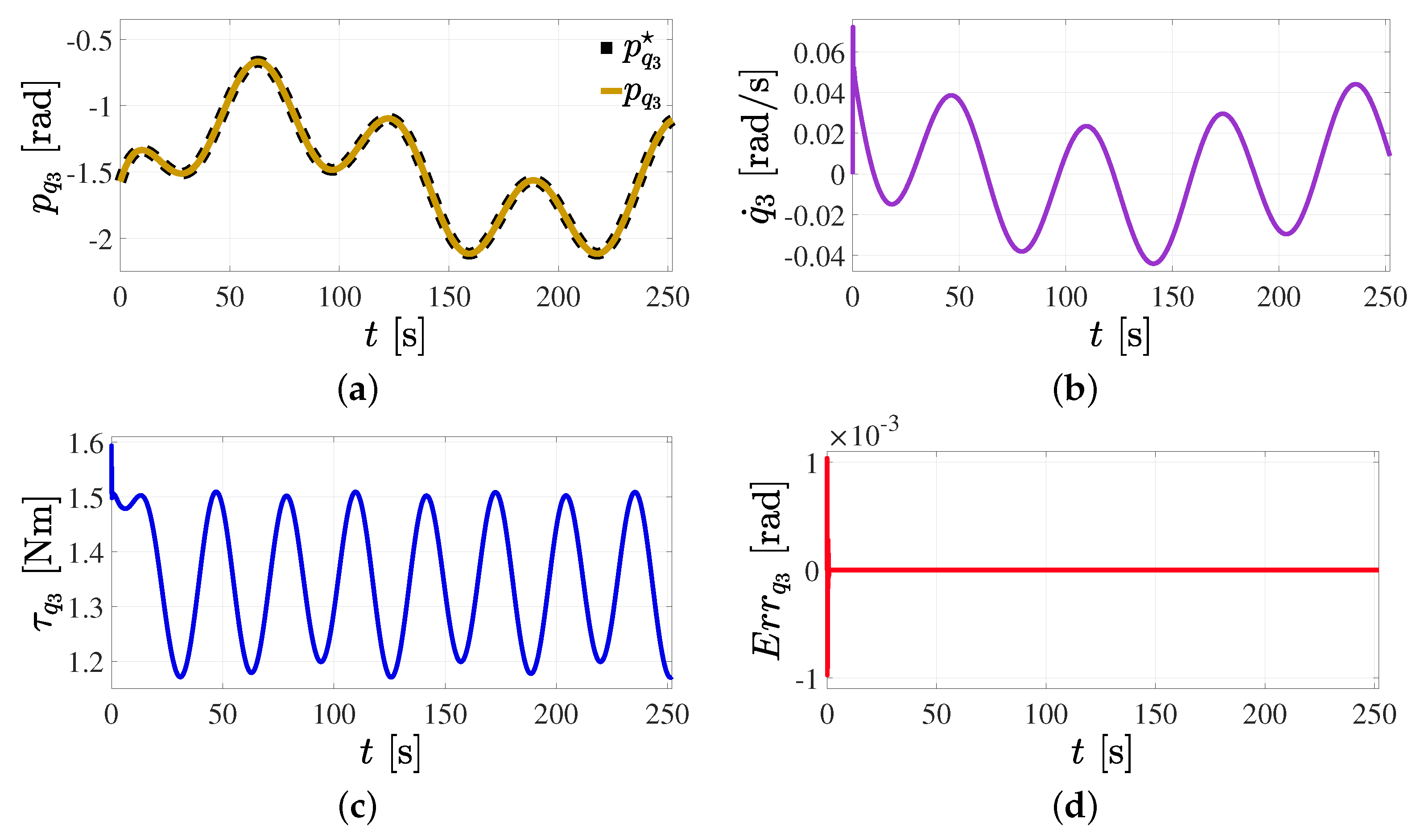
Figure 30 graphically portrays the intricately controlled angular motion of the manipulator robot’s third link within its own joint space. This aspect is crucial, as it represents the final and arguably most essential requirement for the successful execution of the trajectory tracking task, initially outlined in Figure 25. In addition to this, the figure conveniently showcases the angular velocity of the third link that was obtained during the progression of the trajectory tracking task.
It is also worth noting that the three dynamic control parameters corresponding to this variable steadily converge to a steady-state value. This adaptive behavior of the control parameters is a key factor for enabling the task to reach its satisfactory conclusion.

5.4. Trajectory Tracking Control in Cartesian Space with Parameter Variation

The fourth scenario presents the trajectory tracking control of a mobile manipulation robotic system in Cartesian space. The main objective of this case study is to demonstrate the proposed control efficacy for a larger robotic system with a set of parameters different from those presented in Table 2. The main features of the neural adaptive control method based on output feedback for highly nonlinear mobile manipulation robotic systems are numerically confirmed. The values of system parameters and constants used for control robustness simulation analysis are described in Table 3 [70]. Nevertheless, the proposed planned motion trajectory tracking control scheme admits parameters for any realistic application into the operating region specified in the mechatronic design of the robotic system. In contrast to other control design methodologies, the introduced adaptive motion trajectory tracking control design perspective based on B-Spline artificial neural networks and dynamic disturbance compensation reduces the dependency on accurate and detailed knowledge of all multi-input–multi-output nonlinear robotic system parameters considerably. Additional development of effective strategies for accurate real-time estimation of parameters, velocity signals, and time-varying disturbances on multivariable uncertain nonlinear dynamic systems are unnecessary in the presented alternative design approach.
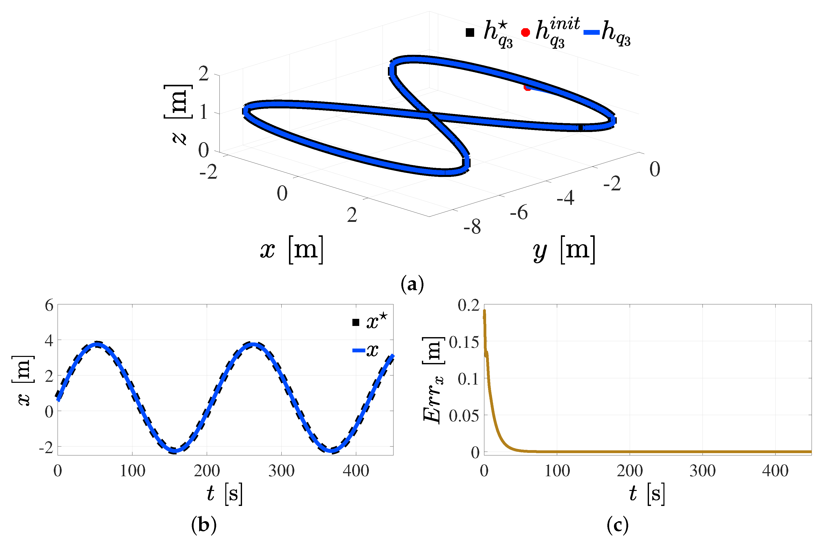
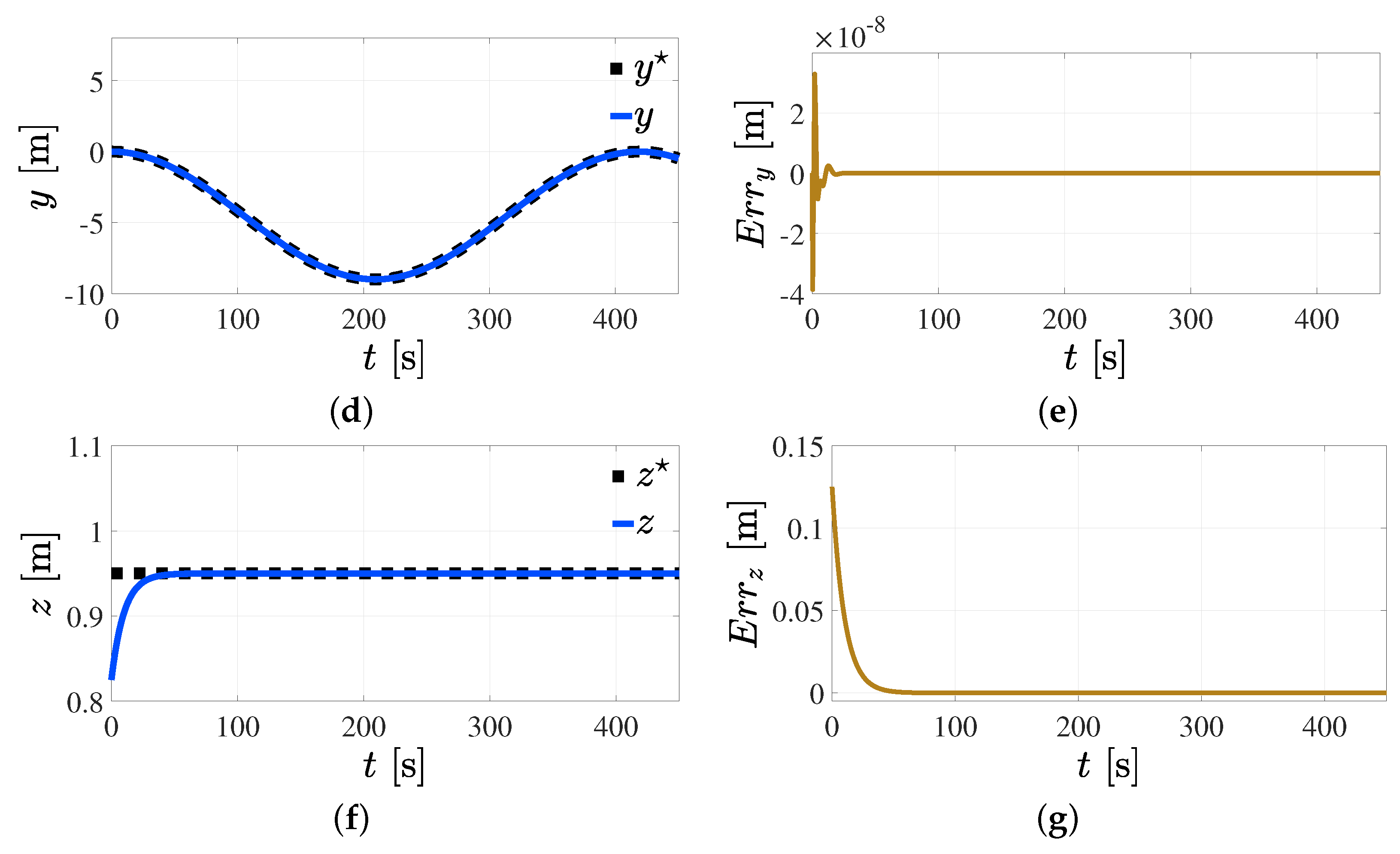
In this scenario, the Cartesian position references h are expressed as follows, with a simulation time of 450 s
x = 0.75 + 3 sin 0.03 t [ m ] y = 4.5 + 4.5 cos 0.015 t [ m ] z = 0.95 [ m ] .
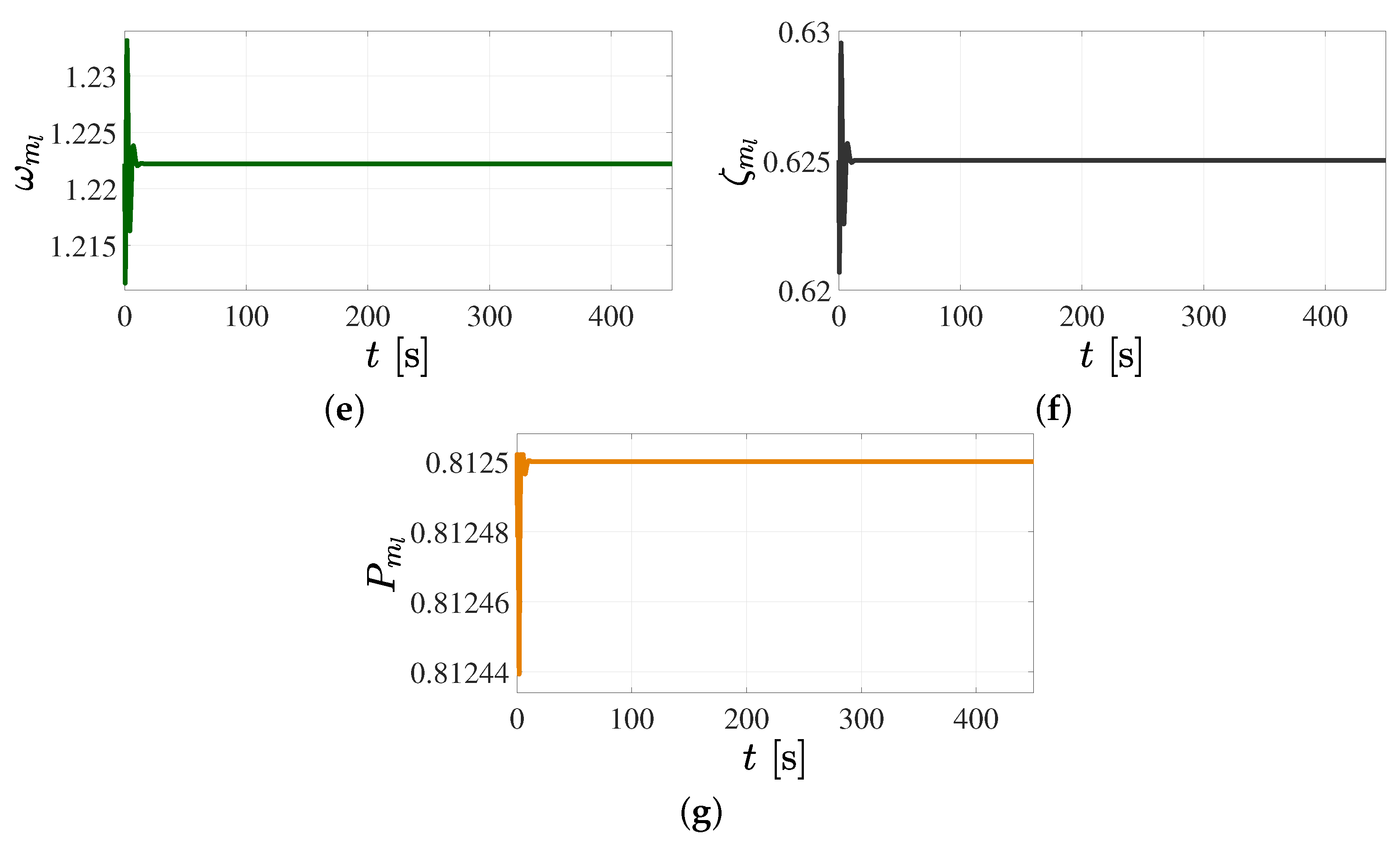
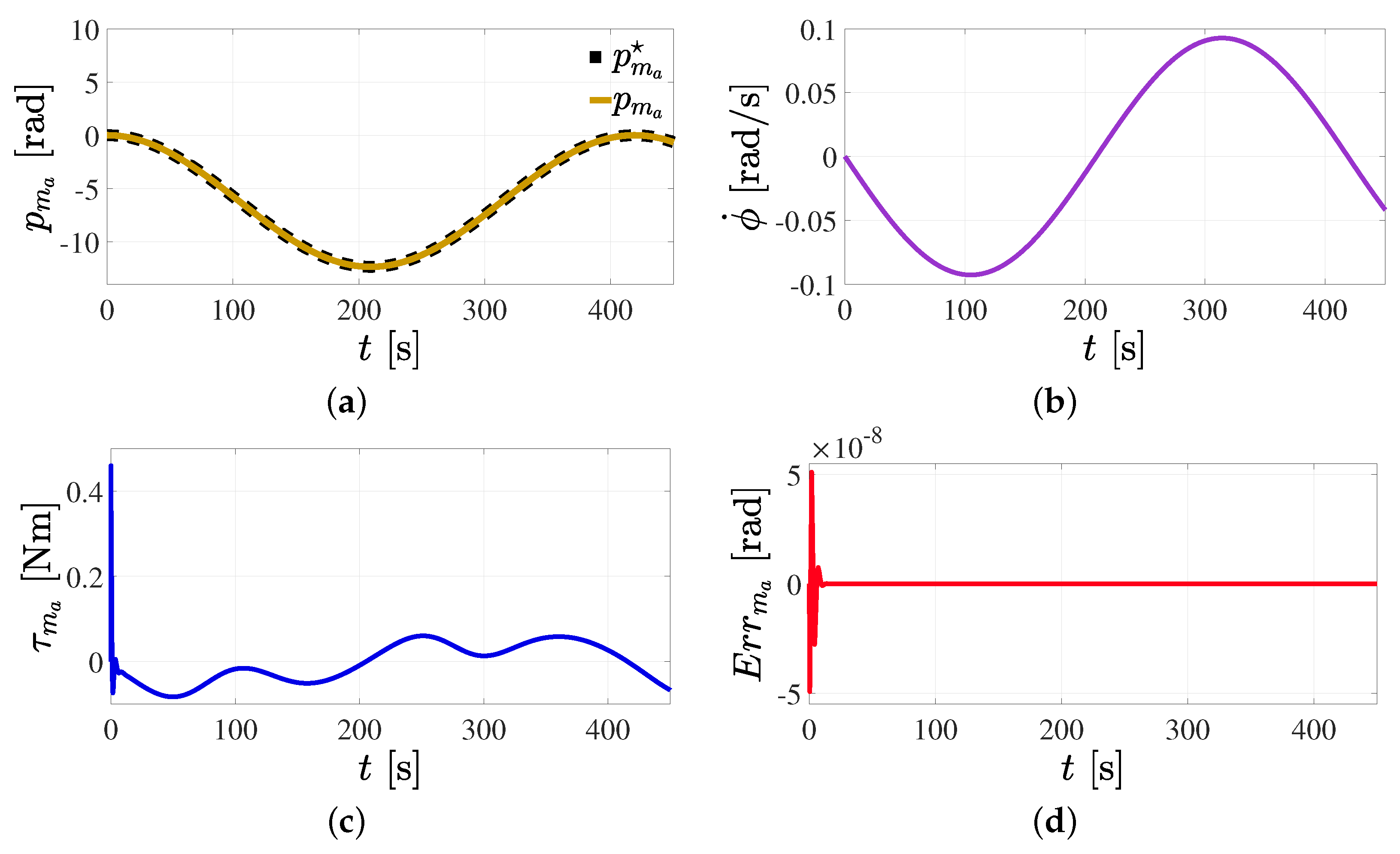
For implementation of the presented neural adaptive control scheme, velocity and acceleration reference trajectories are unnecessary. Moreover, efficient and robust tracking of planned motion reference trajectories Equation (46) should be performed on the controlled mobile manipulation robotic system by using measurements of position signals only. The acceptable control performance of the overall mobile manipulation robotic system for this last operational scenario is depicted in Figure 31, Figure 32, Figure 33, Figure 34, Figure 35 and Figure 36.
Satisfactory control performance in Cartesian space of the mobile manipulation robotic system is revealed in Figure 31. Effective tracking of reference trajectories is clearly evidenced. Furthermore, asymptotic convergence of the tracking errors to zero is confirmed.
Figure 32 presents the controlled linear motion of the mobile robot within its local coordinate frame. The responses of the respective control inputs are depicted. Tuning parameters employing B-Spline artificial neural networks to compute online the control gains are also displayed. The tracking of the position reference trajectory p m l is efficiently executed. Convergence of the trajectory tracking error to zero is similarly achieved.
The effectively controlled angular motion response of the mobile robot within its local coordinate frame is indicated in Figure 33. The control capability to follow the angular position reference trajectory p m a is verified. As shown, the angular position reference trajectory tracking error is asymptotically transferred to zero. The closed-loop angular velocity response and computed driving torque to carry out this specified motion task are portrayed. Fast control parameter adaptation based on B-Spline artificial neural networks can be observed as well.
Figure 34 illustrates the adaptively controlled angular motion of the first link of the manipulator robot within its joint space. Satisfactory tracking of the angular position reference trajectory p q 1 planned for the robot’s first link is corroborated under the influence of the disturbances described in Section 3. Fast neural network tuning of the control parameters ω q 1 (rad/s), ζ q 1 , and P q 1 (rad/s) associated with the desired tracking error dynamics is attained. In this way, appropriate control torque input is exhibited.
The closed-loop angular motion responses of the second link of the uncertain nonlinear manipulator robot are displayed in Figure 35. Robust and efficient dynamic control performance can also be verified. The proposed robust neural control scheme similarly achieves effective tracking of the angular position reference profile given by p q 2 . The asymptotically stable closed-loop trajectory tracking error response associated with the second link of the manipulator robot can be appreciated. Acceptable control torque input response is shown. Indeed, the proposed B-Spline neural network adaptive control architecture avoids adverse high-gain effects to actively suppress disturbances. It can also be observed that the control tuning parameters are efficiently computed online.
Figure 36 graphically portrays the intricately controlled angular motion of the manipulator robot’s third link within its joint space. This represents the final requirement for the successful execution of the tracking task of the motion planning, initially outlined in Figure 26. Adaptive trajectory tracking control dynamic performance using position measurements is again confirmed.
As illustrated in the provided figures within this scenario, the efficacy of the control scheme is evaluated in the face of a collection of numerical parameters that represent a larger system than initially contemplated. Upon scrutinizing these results, it is observed that the real-time adjustment of the dynamic control parameters facilitates the generation of low-magnitude control signals. Likewise, the control velocities manifested are of relatively diminutive magnitude, thereby ensuring smooth motion that maintains the system’s stability throughout the task execution process. This indicates well-modulated, controlled operation, safeguarding against abrupt fluctuations that could potentially destabilize the system.

6. Conclusions

This research delved into the complexities of controlling the motion of a mobile manipulation robotic system by employing B-Spline artificial neural networks. This innovative approach to motion control delivered robust and adaptive results in the regulation and tracking of both linear and angular motion through rigorous simulation experiments and extensive analysis. The implementation of the B-Spline artificial neural networks as an integral part of the control scheme showcased their remarkable effectiveness in mitigating challenges. Their proficiency was evident when addressing issues related to both the differential-drive mobile robot and the anthropomorphic manipulator robot. For the mobile robot, the control scheme ensured regulated linear and angular motion within its local coordinate frame, a critical necessity for trajectory tracking tasks. Meanwhile, for the manipulator robot, the control scheme facilitated proficient management of angular motion within the joint space across its three links, underscoring its importance for successful task completion. A salient feature of B-Spline artificial neural networks is their dynamic adaptability and learning capacity, which found expression in the controllers’ ability to stabilize control parameters to a constant value. This ability proved instrumental to ensuring task completion despite unforeseen external disturbances. Furthermore, the control scheme demonstrated resilience to unexpected environmental changes and scalable, adaptable capacity to handle robotic systems with varying degrees of freedom, highlighting the substantial potential of B-Spline neural networks in motion control. The control scheme also excelled in tracking desired position profiles with high precision, even when confronted with induced external vibratory torques, illustrating its robust nature. Its adaptability, as evidenced by the stable response to continuous changes to position profiles, is invaluable in dynamic and unpredictable work environments. An in-depth examination of the control scheme’s minimal numerical output for both force and torque emphasizes its efficiency. This level of efficiency, despite considerable magnitudes of disturbance forces and torques, not only validates the control scheme’s proficiency but also precludes actuator saturation, extending the operational lifespan of the system. Adaptive neural-network robust control of other architectures of mobile manipulation robotic systems for special application scenarios of large-scale manufacturing under substantially disturbed operational environments will be developed in future research work. In this sense, several experimental and numerical comparative analysis case studies of different methods will be introduced in subsequent contributions as well.

Author Contributions

Conceptualization, D.G.-P., F.B.-C., I.R.-C., H.Y.-B., A.F.-C. and R.T.-O.; Data curation, D.G.-P. and H.Y.-B.; Formal analysis, D.G.-P., F.B.-C., H.Y.-B., I.R.-C., A.F.-C. and R.T.-O.; Investigation, D.G.-P., F.B.-C., I.R.-C., H.Y.-B., A.F.-C. and R.T.-O.; Methodology, D.G.-P., F.B.-C., I.R.-C., H.Y.-B., A.F.-C. and R.T.-O.; Project administration, F.B.-C.; Software, D.G.-P. and H.Y.-B.; Supervision, F.B.-C. and I.R.-C.; Validation, D.G.-P. and H.Y.-B.; Writing—original draft, D.G.-P., F.B.-C. and H.Y.-B.; Writing—review and editing, D.G.-P., F.B.-C., I.R.-C., H.Y.-B., A.F.-C. and R.T.-O. All authors have read and agreed to the published version of the manuscript.

Funding

This research received no external funding.

Data Availability Statement

Not applicable.

Acknowledgments

The authors would like to thank Consejo Nacional de Humanidades, Ciencias y Tecnologías (CONAHCYT) for support given to developing this work.

Conflicts of Interest

The authors declare no conflict of interest.

Abbreviations

The following abbreviations are used in this manuscript:
ANNArtificial Neural Network
BS-ANNB-Spline Artificial Neural Network
DCDirect Current
DOFDegrees of Freedom
PDProportional Derivative
PIDProportional Integral Derivative

References

  1. Dörfler, K.; Dielemans, G.; Lachmayer, L.; Recker, T.; Raatz, A.; Lowke, D.; Gerke, M. Additive Manufacturing using Mobile Robots: Opportunities and Challenges for Building Construction. Cem. Concr. Res. 2022, 158, 106772. [Google Scholar] [CrossRef]
  2. Matheson, E.; Minto, R.; Zampieri, E.G.; Faccio, M.; Rosati, G. Human–Robot Collaboration in Manufacturing Applications: A Review. Robotics 2019, 8, 100. [Google Scholar] [CrossRef] [Green Version]
  3. Wilson, M. Industrial Robots. In Implementation of Robot Systems: An Introduction to Robotics, Automation, and Successful Systems Integration in Manufacturing; Butterworth-Heinemann: London, UK, 2014; pp. 19–38. [Google Scholar]
  4. Sandakalum, T.; Ang Jr, M.H. Motion Planning for Mobile Manipulators—A Systematic Review. Machines 2022, 10, 97. [Google Scholar] [CrossRef]
  5. Bonci, A.; Cen Cheng, P.D.; Indri, M.; Nabissi, G.; Sibona, F. Human–Robot Perception in Industrial Environments: A Survey. Sensors 2021, 21, 1571. [Google Scholar] [CrossRef]
  6. Yang, M.; Yang, E.; Zante, R.C.; Post, M.; Liu, X. Collaborative Mobile Industrial Manipulator: A Review of System Architecture and Applications. In Proceedings of the 2019 25th International Conference on Automation and Computing (ICAC 2019), Lancaster, UK, 5–7 September 2019; pp. 1–6. [Google Scholar]
  7. Li, R.; Qiao, H. A Survey of Methods and Strategies for High–Precision Robotic Grasping and Assembly Tasks—Some New Trends. IEEE/ASME Trans. Mechatronics 2019, 24, 2718–2732. [Google Scholar] [CrossRef]
  8. Sumanas, M.; Petronis, A.; Bucinskas, V.; Dzedzickis, A.; Virzonis, D.; Morkvenaite-Vilkonciene, I. Deep Q–Learning in Robotics: Improvement of Accuracy and Repeatability. Sensors 2022, 22, 3911. [Google Scholar] [CrossRef] [PubMed]
  9. Arents, J.; Greitans, M. Smart Industrial Robot Control Trends, Challenges and Opportunities within Manufacturing. Appl. Sci. 2022, 12, 937. [Google Scholar] [CrossRef]
  10. Liu, Z.; Liu, Q.; Xu, W.; Wang, L.; Zhou, Z. Robot Learning towards Smart Robotic Manufacturing: A Review. Robot. Comput.-Integr. Manuf. 2022, 77, 102360. [Google Scholar] [CrossRef]
  11. Liu, H.; Wang, L. Remote Human–Robot Collaboration: A Cyber–Physical System Application for Hazard Manufacturing Environment. J. Manuf. Syst. 2020, 54, 24–34. [Google Scholar] [CrossRef]
  12. Oomen, T. Advanced Motion Control for Precision Mechatronics: Control, Identification, and Learning of Complex Systems. Ieej J. Ind. Appl. 2018, 7, 127–140. [Google Scholar] [CrossRef] [Green Version]
  13. Hamner, B.; Koterba, S.; Shi, J.; Simmons, R.; Singh, S. An Autonomous Mobile Manipulator for Assembly Tasks. Auton. Robot. 2010, 28, 131–149. [Google Scholar] [CrossRef]
  14. Alandoli, E.A.; Lee, T.; Vijayakumar, V.; Lin, Y.; Mohammed, M.Q. Dynamic Model and Integrated Optimal Controller of Hybrid Arms Robot for Laser Contour Machining. J. Vib. Control 2022, 29, 10775463221090000. [Google Scholar] [CrossRef]
  15. Jafari, D.; Vaneker, T.H.; Gibson, I. Wire and Arc Additive Manufacturing: Opportunities and Challenges to Control the Quality and Accuracy of Manufactured Parts. Mater. Des. 2021, 202, 109471. [Google Scholar] [CrossRef]
  16. Nagabandi, A.; Konolige, K.; Levine, S.; Kumar, V. Deep Dynamics Models for Learning Dexterous Manipulation. In Proceedings of the Conference on Robot Learning, Virtual Event, 16–18 November 2020; pp. 1101–1112. [Google Scholar]
  17. Billard, A.; Kragic, D. Trends and Challenges in Robot Manipulation. Science 2019, 364, eaat8414. [Google Scholar] [CrossRef]
  18. Kumar, M.; Shenbagaraman, V.; Shaw, R.N.; Ghosh, A. Digital Transformation in Smart Manufacturing with Industrial Robot through Predictive Data Analysis. In Machine Learning for Robotics Applications; Springer: Singapore, 2021; pp. 85–105. [Google Scholar]
  19. Javaid, M.; Haleem, A.; Singh, R.P.; Suman, R. Substantial Capabilities of Robotics in Enhancing Industry 4.0 Implementation. Cogn. Robot. 2021, 1, 58–75. [Google Scholar] [CrossRef]
  20. Beschi, M.; Mutti, S.; Nicola, G.; Faroni, M.; Magnoni, P.; Villagrossi, E.; Pedrocchi, N. Optimal Robot Motion Planning of Redundant Robots in Machining and Additive Manufacturing Applications. Electronics 2019, 8, 1437. [Google Scholar] [CrossRef] [Green Version]
  21. Bi, Z.M.; Luo, C.; Miao, Z.; Zhang, B.; Zhang, W.; Wang, L. Safety Assurance Mechanisms of Collaborative Robotic Systems in Manufacturing. Robot. Comput.-Integr. Manuf. 2021, 67, 102022. [Google Scholar] [CrossRef]
  22. Minniti, M.V.; Farshidian, F.; Grandia, R.; Hutter, M. Whole–Body MPC for a Dynamically Stable Mobile Manipulator. IEEE Robot. Autom. Lett. 2019, 4, 3687–3694. [Google Scholar] [CrossRef] [Green Version]
  23. Garnier, S.; Subrin, K.; Arevalo-Siles, P.; Caverot, G.; Furet, B. Mobile Robot Stability for Complex Tasks in Naval Industries. Procedia CIRP 2018, 72, 297–302. [Google Scholar] [CrossRef]
  24. Zacharaki, A.; Kostavelis, I.; Gasteratos, A.; Dokas, I. Safety Bounds in Human Robot Interaction: A Survey. Saf. Sci. 2020, 127, 104667. [Google Scholar] [CrossRef]
  25. Fareh, R.; Khadraoui, S.; Abdallah, M.Y.; Baziyad, M.; Bettayeb, M. Active Disturbance Rejection Control for Robotic Systems: A Review. Mechatronics 2021, 80, 102671. [Google Scholar] [CrossRef]
  26. Liu, S.; Wang, L.; Wang, X.V. Sensorless Force Estimation for Industrial Robots using Disturbance Observer and Neural Learning of Friction Approximation. Robot. Comput.-Integr. Manuf. 2021, 71, 102168. [Google Scholar] [CrossRef]
  27. Nikranjbar, A.; Haidari, M.; Atai, A.A. Adaptive Sliding Mode Tracking Control of Mobile Robot in Dynamic Environment using Artificial Potential Fields. J. Comput. Robot. 2018, 11, 1–14. [Google Scholar]
  28. Katz, D.; Horrell, E.; Yang, Y.; Burns, B.; Buckley, T.; Grishkan, A.; Zhylkovskyy, V.; Brock, O.; Learned-Miller, E. The UMass Mobile Manipulator UMan: An Experimental Platform for Autonomous Mobile Manipulation. In Workshop on Manipulation in Human Environments at Robotics: Science and Systems; University of Pennsylvania: Philadelphia, PA, USA, 2006; Available online: https://people.cs.umass.edu/~elm/papers/UMan_workshop_06.pdf (accessed on 25 June 2023).
  29. Ambrose, R.O.; Savely, R.T.; Goza, S.M.; Strawser, P.; Diftler, M.A.; Spain, I.; Radford, N. Mobile Manipulation using NASA’s Robonaut. In Proceedings of the IEEE International Conference on Robotics and Automation, 2004. Proceedings. ICRA’04. 2004, New Orleans, LA, USA, 26 April–1 May 2004; Volume 2, pp. 2104–2109. [Google Scholar]
  30. Park, D.; Hoshi, Y.; Mahajan, H.P.; Kim, H.K.; Erickson, Z.; Rogers, W.A.; Kemp, C.C. Active Robot–Assisted Feeding with a General-Purpose Mobile Manipulator: Design, Evaluation, and Lessons Learned. Robot. Auton. Syst. 2020, 124, 103344. [Google Scholar] [CrossRef]
  31. Yamamoto, T.; Terada, K.; Ochiai, A.; Saito, F.; Asahara, Y.; Murase, K. Development of Human Support Robot as the Research Platform of a Domestic Mobile Manipulator. Robomech J. 2019, 6, 4. [Google Scholar] [CrossRef] [Green Version]
  32. Merckaert, K.; Convens, B.; Wu, C.-j.; Roncone, A.; Nicotra, M.M.; Vanderborght, B. Real–Time Motion Control of Robotic Manipulators for Safe Human–Robot Coexistence. Robot. Comput.-Integr. Manuf. 2022, 73, 102223. [Google Scholar] [CrossRef]
  33. Prasad, A.; Sharma, B.; Vanualailai, J.; Kumar, S. Motion Control of an Articulated Mobile Manipulator in 3D using the Lyapunov–based Control Scheme. Int. J. Control 2022, 95, 2581–2595. [Google Scholar] [CrossRef]
  34. Fareh, R.; Saad, M.R.; Saad, M.; Brahmi, A.; Bettayeb, M. Trajectory Tracking and Stability Analysis for Mobile Manipulators based on Decentralized Control. Robotica 2019, 37, 1732–1749. [Google Scholar] [CrossRef]
  35. Brahmi, A.; Saad, M.; Brahmi, B.; Bojairami, I.E.; Gauthier, G.; Ghommam, J. Robust Adaptive Tracking Control for Uncertain Nonholonomic Mobile Manipulator. Proc. Inst. Mech. Eng. Part J. Syst. Control Eng. 2022, 236, 395–405. [Google Scholar] [CrossRef]
  36. Mishra, S.; Londhe, P.S.; Mohan, S.; Vishvakarma, S.K.; Patre, B. Robust Task–Space Motion Control of a Mobile Manipulator using a Nonlinear Control with an Uncertainty Estimator. Comput. Electr. Eng. 2018, 67, 729–740. [Google Scholar] [CrossRef]
  37. Xia, K.; Gao, H.; Ding, L.; Liu, G.; Deng, Z.; Liu, Z.; Ma, C. Trajectory Tracking Control of Wheeled Mobile Manipulator based on Fuzzy Neural Network and Extended Kalman Filtering. Neural Comput. Appl. 2018, 30, 447–462. [Google Scholar] [CrossRef]
  38. Mai, T. Hybrid Adaptive Tracking Control Method for Mobile Manipulator Robot based on Proportional–Integral–Derivative Technique. Proc. Inst. Mech. Eng. Part J. Mech. Eng. Sci. 2021, 235, 6463–6480. [Google Scholar] [CrossRef]
  39. Qin, D.; Liu, A.; Xu, J.; Zhang, W.A.; Yu, L. Learning from Human Demonstrations for Wheel Mobile Manipulator: An Unscented Model Predictive Control Approach. IEEE Trans. Neural Netw. Learn. Syst. 2022. early access. [Google Scholar] [CrossRef]
  40. Liu, L.; Yue, X.; Wen, H.; Hao, Z.; Wang, Z. Output Feedback Tracking Control for Nonholonomic Wheeled Mobile Manipulator Systems with Full–Output Constraints. Proc. Inst. Mech. Eng. Part J. Syst. Control Eng. 2023, 237, 09596518221141489. [Google Scholar] [CrossRef]
  41. Sharma, M.; Luthra, S.; Joshi, S.; Kumar, A. Implementing Challenges of Artificial Intelligence: Evidence from Public Manufacturing Sector of an Emerging Economy. Gov. Inf. Q. 2022, 39, 101624. [Google Scholar] [CrossRef]
  42. Arinez, J.F.; Chang, Q.; Gao, R.X.; Xu, C.; Zhang, J. Artificial Intelligence in Advanced Manufacturing: Current Status and Future Outlook. J. Manuf. Sci. Eng. 2020, 142, 110804. [Google Scholar] [CrossRef]
  43. Balamurugan, E.; Flaih, L.R.; Yuvaraj, D.; Sangeetha, K.; Jayanthiladevi, A.; Kumar, T.S. Use Case of Artificial Intelligence in Machine Learning Manufacturing 4.0. In Proceedings of the 2019 International conference on computational intelligence and knowledge economy (ICCIKE), Dubai, United Arab Emirates, 11–12 December 2019; pp. 656–659. [Google Scholar]
  44. Soori, M.; Arezoo, B.; Dastres, R. Artificial Intelligence, Machine Learning and Deep Learning in Advanced Robotics, A Review. Cogn. Robot. 2023, 3, 54–70. [Google Scholar] [CrossRef]
  45. Kim, S.W.; Kong, J.H.; Lee, S.W.; Lee, S. Recent Advances of Artificial Intelligence in Manufacturing Industrial Sectors: A Review. Int. J. Precis. Eng. Manuf. 2022, 23, 111–129. [Google Scholar] [CrossRef]
  46. Xiao, H.; Muthu, B.; Kadry, S.N. Artificial Intelligence with Robotics for Advanced Manufacturing Industry using Robot–Assisted Mixed–Integer Programming Model. Intell. Serv. Robot. 2020, 1–10. [Google Scholar] [CrossRef]
  47. Saridis, G. Intelligent Robotic Control. IEEE Trans. Autom. Control 1983, 28, 547–557. [Google Scholar] [CrossRef]
  48. de Silva, C.W. Intelligent Control of Robotic Systems with Application in Industrial Processes. Robot. Auton. Syst. 1997, 21, 221–237. [Google Scholar] [CrossRef]
  49. Rawat, D.; Gupta, M.K.; Sharma, A. Intelligent Control of Robotic Manipulators: A Comprehensive Review. Spat. Inf. Res. 2022, 31, 345–357. [Google Scholar] [CrossRef]
  50. Jin, L.; Li, S.; Yu, J.; He, J. Robot Manipulator Control using Neural Networks: A Survey. Neurocomputing 2018, 285, 23–34. [Google Scholar] [CrossRef]
  51. Montesinos López, O.A.; Montesinos López, A.; Crossa, J. Fundamentals of Artificial Neural Networks and Deep Learning. In Multivariate Statistical Machine Learning Methods for Genomic Prediction; Springer: Cham, Switzerland, 2022; pp. 379–425. [Google Scholar]
  52. Chaoui, H.; Sicard, P.; Gueaieb, W. ANN–based Adaptive Control of Robotic Manipulators with Friction and Joint Elasticity. IEEE Trans. Ind. Electron. 2009, 56, 3174–3187. [Google Scholar] [CrossRef]
  53. Wai, R.J. Tracking Control based on Neural Network Strategy for Robot Manipulator. Neurocomputing 2003, 51, 425–445. [Google Scholar] [CrossRef]
  54. Liu, Z.; Peng, K.; Han, L.; Guan, S. Modeling and Control of Robotic Manipulators Based on Artificial Neural Networks: A Review. Iran. J. Sci. Technol. Trans. Mech. Eng. 2023, 1–41. [Google Scholar] [CrossRef]
  55. Yen, V.T.; Nan, W.Y.; Van Cuong, P. Robust Adaptive Sliding Mode Neural Networks Control for Industrial Robot Manipulators. Int. J. Control. Autom. Syst. 2019, 17, 783–792. [Google Scholar] [CrossRef]
  56. Miljković, Z.; Mitić, M.; Lazarević, M.; Babić, B. Neural Network Reinforcement Learning for Visual Control of Robot Manipulators. Expert Syst. Appl. 2013, 40, 1721–1736. [Google Scholar] [CrossRef]
  57. Sun, Y.; Gao, Y.; Zhao, Y.; Liu, Z.; Wang, J.; Kuang, J.; Yan, F.; Liu, J. Neural Network–based Tracking Control of Uncertain Robotic Systems: Predefined–Time Nonsingular Terminal Sliding–Mode Approach. IEEE Trans. Ind. Electron. 2022, 69, 10510–10520. [Google Scholar] [CrossRef]
  58. Han, N.; Ren, X.; Zhang, C.; Zheng, D. Prescribed Performance Control with Input Indicator for Robot System based on Spectral Normalized Neural Networks. Neurocomputing 2022, 492, 201–210. [Google Scholar] [CrossRef]
  59. Yañez-Badillo, H.; Beltran-Carbajal, F.; Tapia-Olvera, R.; Favela-Contreras, A.; Sotelo, C.; Sotelo, D. Adaptive Robust Motion Control of Quadrotor Systems using Artificial Neural Networks and Particle Swarm Optimization. Mathematics 2021, 9, 2367. [Google Scholar] [CrossRef]
  60. Yañez-Badillo, H.; Tapia-Olvera, R.; Beltran-Carbajal, F. Adaptive Neural Motion Control of a Quadrotor UAV. Vehicles 2020, 2, 468–490. [Google Scholar] [CrossRef]
  61. Yañez Badillo, H.; Tapia Olvera, R.; Aguilar Mejía, O.; Beltrán Carbajal, F. Control Neuronal en Línea para Regulación y Seguimiento de Trayectorias de Posición para un Quadrotor. Rev. Iberoam. Autom. Inform. Ind. 2017, 14, 141–151. [Google Scholar] [CrossRef] [Green Version]
  62. Galvan-Perez, D.; Yañez-Badillo, H.; Beltran-Carbajal, F.; Rivas-Cambero, I.; Favela-Contreras, A.; Tapia-Olvera, R. Neural Adaptive Robust Motion–Tracking Control for Robotic Manipulator Systems. Actuators 2022, 11, 255. [Google Scholar] [CrossRef]
  63. Beltran-Carbajal, F.; Tapia-Olvera, R.; Valderrabano-Gonzalez, A.; Lopez-Garcia, I. Adaptive Neuronal Induction Motor Control with an 84–Pulse Voltage Source Converter. Asian J. Control 2021, 23, 1603–1616. [Google Scholar] [CrossRef]
  64. Beltran-Carbajal, F.; Tapia-Olvera, R.; Lopez-Garcia, I.; Guillen, D. Adaptive Dynamical Tracking Control under Uncertainty of Shunt DC Motors. Electr. Power Syst. Res. 2018, 164, 70–78. [Google Scholar] [CrossRef]
  65. Lin, Z.; Reay, D.S.; Williams, B.W.; He, X. Online Modeling for Switched Reluctance Motors using B–Spline Neural Networks. IEEE Trans. Ind. Electron. 2007, 54, 3317–3322. [Google Scholar] [CrossRef]
  66. Tapia-Olvera, R.; Beltran-Carbajal, F.; Valderrabano-Gonzalez, A. Adaptive Neural Trajectory Tracking Control for Synchronous Generators in Interconnected Power Systems. Appl. Sci. 2022, 13, 561. [Google Scholar] [CrossRef]
  67. Beltran-Carbajal, F.; Yañez-Badillo, H.; Tapia-Olvera, R.; Rosas-Caro, J.C.; Sotelo, C.; Sotelo, D. Neural Network Trajectory Tracking Control on Electromagnetic Suspension Systems. Mathematics 2023, 11, 2272. [Google Scholar] [CrossRef]
  68. Varela-Aldás, J.; Andaluz, V.H.; Chicaiza, F.A. Modelling and Control of a Mobile manipulator for Trajectory Tracking. In Proceedings of the 2018 International Conference on Information Systems and Computer Science (INCISCOS), Quito, Ecuador, 13–15 November 2018; pp. 69–74. [Google Scholar]
  69. Prada-Jiménez, V.; Niño-Suárez, P.A.; Mauledoux-Monroy, M.F.; Aponte-Rodríguez, J. Coupled Dynamic Model for a Mobile Manipulator. Int. J. Appl. Eng. Res. 2019, 14, 2622–2629. [Google Scholar]
  70. Prada-Jimenez, V.; Niáo-Suaréz, P.A.; Portilla-Flores, E.A.; Mauledoux-Monroy, M.F. Tuning a PD+ Controller by Means of Dynamic Optimization in a Mobile Manipulator with Coupled Dynamics. IEEE Access 2019, 7, 124712–124726. [Google Scholar] [CrossRef]
  71. Li, Z.; Ge, S.S.; Adams, M.; Wijesoma, W.S. Adaptive Robust Output–Feedback Motion/Force Control of Electrically Driven Nonholonomic Mobile Manipulators. IEEE Trans. Control Syst. Technol. 2008, 16, 1308–1315. [Google Scholar]
  72. Moon, F.C. Applied Dynamics: With Applications to Multibody and Mechatronic Systems; John Wiley & Sons: Hoboken, NJ, USA, 2008. [Google Scholar]
  73. Cortés, F.R. Dinámica de Robots Manipuladores. In Robótica: Control de Robots Manipuladores; Marcombo: Barcelona, Spain, 2020; pp. 259–263. (In Spanish) [Google Scholar]
  74. Li, Z.; Ming, A.; Xi, N.; Shimojo, M. Motion Control of Nonholonomic Mobile Underactuated Manipulator. In Proceedings of the Proceedings 2006 IEEE International Conference on Robotics and Automation, 2006. ICRA, Orlando, FL, USA, 15–19 May 2006; pp. 3512–3519. [Google Scholar]
  75. Li, Z.; Gu, J.; Ming, A.; Xu, C.; Shimojo, M. Intelligent Compliant Force/Motion Control of Nonholonomic Mobile Manipulator Working on the Nonrigid Surface. Neural Comput. Appl. 2006, 15, 204–216. [Google Scholar] [CrossRef]
  76. Jia, Y.; Xi, N.; Cheng, Y.; Liang, S. Coordinated Motion Control of a Nonholonomic Mobile Manipulator for Accurate Motion Tracking. In Proceedings of the 2014 IEEE/RSJ International Conference on Intelligent Robots and Systems, Chicago, IL, USA, 14–18 September 2014; pp. 1635–1640. [Google Scholar]
  77. Fliess, M.; Marquez, R.; Delaleau, E.; Sira-Ramírez, H. Correcteurs Proportionnels–Intégraux Généralisés. Esaim Control. Optim. Calc. Var. 2002, 7, 23–41. [Google Scholar] [CrossRef] [Green Version]
  78. Haykin, S. Neural Networks and Learning Machines; Pearson: London, UK, 2009. [Google Scholar]
  79. Bossley, K.; Brown, M.; Harris, C. Neurofuzzy Adaptive Modelling and Construction of Nonlinear Dynamical Processes. Neural Network Applications in Control; Institution of Engineering and Technology (IET): Stevenage, UK, 1995; pp. 253–292. [Google Scholar]
  80. Harris, C.J.; Moore, C.G.; Brown, M. Intelligent Control: Aspects of Fuzzy Logic and Neural Nets; World Scientific: London, UK, 1993. [Google Scholar]
  81. dos Santos Coelho, L.; Pessôa, M.W. Nonlinear Identification using a B–Spline Neural Network and Chaotic Immune Approaches. Mech. Syst. Signal Process. 2009, 23, 2418–2434. [Google Scholar] [CrossRef]
  82. Oliveira, T.R.; Peixoto, A.J.; Nunes, E.V. Binary Robust Adaptive Control with Monitoring Functions for Systems under Unknown High–Frequency–Gain Sign, Parametric Uncertainties and Unmodeled Dynamics. Int. J. Adapt. Control Signal Process. 2016, 30, 1184–1202. [Google Scholar] [CrossRef]
  83. Yao, J.; Deng, W. Active Disturbance Rejection Adaptive Control of Uncertain Nonlinear Systems: Theory and Application. Nonlinear Dynamics 2017, 89, 1611–1624. [Google Scholar] [CrossRef]
  84. Yang, J.; Na, J.; Gao, G. Robust Model Reference Adaptive Control for Transient Performance Enhancement. Int. J. Robust Nonlinear Control 2020, 30, 6207–6228. [Google Scholar] [CrossRef]
  85. Saad, D. On–Line Learning in Neural Networks; Cambridge University Press: Cambridge, UK, 1999. [Google Scholar]
  86. Beltran-Carbajal, F.; Silva-Navarro, G. Output Feedback Dynamic Control for Trajectory Tracking and Vibration Suppression. Appl. Math. Model. 2020, 79, 793–808. [Google Scholar] [CrossRef]
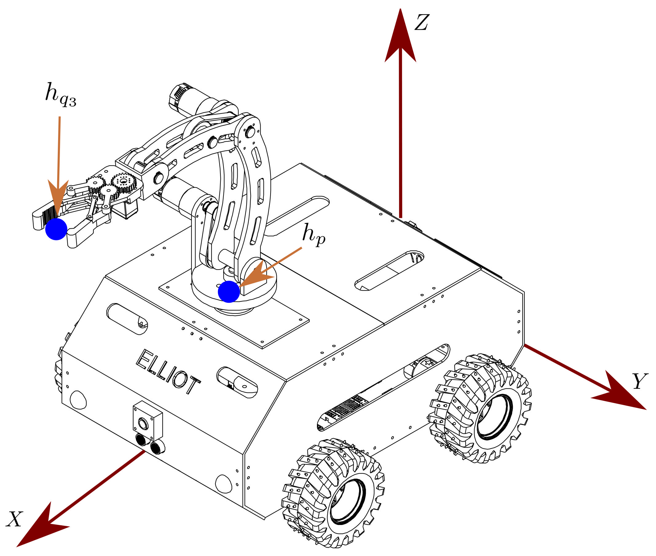
Figure 1. Mobile manipulation robotic system considered in the present study.
Mathematics 11 03489 g001
Figure 2. Projection on XZ-plane displaying a lateral view of the manipulator robot.
Mathematics 11 03489 g002
Figure 3. Projection on XY-plane depicting a superior view of the mobile manipulator robot.
Mathematics 11 03489 g003
Figure 4. Projection on XZ-plane showing a lateral view of the mobile robot.
Mathematics 11 03489 g004
Figure 5. B-Spline artificial-neural-network-based motion-control scheme.
Mathematics 11 03489 g005
Figure 6. B-Spline artificial neural network architecture (BS-ANN).
Mathematics 11 03489 g006
Figure 7. Motion-control scheme of the mobile manipulation robotic system in the joint space.
Mathematics 11 03489 g007
Figure 8. Controlled linear motion of the mobile robot in its local coordinate frame. (a) Controlled linear position p m l . (b) Computed driving force F m l . (c) Linear position error E r r m l . (d) Adaptive ω m l control parameter. (e) Adaptive ζ m l control parameter. (f) Adaptive P m l control parameter.
Mathematics 11 03489 g008aMathematics 11 03489 g008b
Figure 9. Controlled angular motion of the mobile robot in its local coordinate frame. (a) Controlled angular position p m a . (b) Computed driving torque τ m a . (c) Angular position error E r r m a . (d) Adaptive ω m a control parameter. (e) Adaptive ζ m a control parameter. (f) Adaptive P m a control parameter.
Mathematics 11 03489 g009aMathematics 11 03489 g009b
Figure 10. Controlled angular motion of the manipulator robot in its joint space. (a) Controlled angular position p q 1 . (b) Computed driving torque τ q 1 . (c) Angular position error E r r q 1 . (d) Adaptive ω q 1 control parameter. (e) Adaptive ζ q 1 control parameter. (f) Adaptive P q 1 control parameter.
Mathematics 11 03489 g010
Figure 11. Controlled angular motion of the manipulator robot in its joint space. (a) Controlled angular position p q 2 . (b) Computed driving torque τ q 2 . (c) Angular position error E r r q 2 . (d) Adaptive ω q 2 control parameter. (e) Adaptive ζ q 2 control parameter. (f) Adaptive P q 2 control parameter.
Mathematics 11 03489 g011
Figure 12. Controlled angular motion of the manipulator robot in its joint space. (a) Controlled angular position p q 3 . (b) Computed driving torque τ q 3 . (c) Angular position error E r r q 3 . (d) Adaptive ω q 3 control parameter. (e) Adaptive ζ q 3 control parameter. (f) Adaptive P q 3 control parameter.
Mathematics 11 03489 g012
Figure 13. Induced external vibratory torques. (a) Vibratory force F d L . (b) Vibratory torque τ d A . (c) Vibratory torque τ d 1 . (d) Vibratory torque τ d 2 . (e) Vibratory torque τ d 3 .
Mathematics 11 03489 g013
Figure 14. Controlled linear motion of the mobile robot in its local coordinate frame subjected to the external force F d L . (a) Controlled linear position p m l . (b) Computed driving force F m l . (c) Linear position error E r r m l . (d) Adaptive ω m l control parameter. (e) Adaptive ζ m l control parameter. (f) Adaptive P m l control parameter.
Mathematics 11 03489 g014
Figure 15. Controlled angular motion of the mobile robot in its local coordinate frame subjected to the external torque τ d A . (a) Controlled angular position p m a . (b) Computed driving torque τ m a . (c) Angular position error E r r m a . (d) Adaptive ω m a control parameter. (e) Adaptive ζ m a control parameter. (f) Adaptive P m a control parameter.
Mathematics 11 03489 g015aMathematics 11 03489 g015b
Figure 16. Controlled angular motion of the manipulator robot in its joint space subjected to the external torque τ d 1 . (a) Controlled angular position p q 1 . (b) Computed driving torque τ q 1 . (c) Angular position error E r r q 1 . (d) Adaptive ω q 1 control parameter. (e) Adaptive ζ q 1 control parameter. (f) Adaptive P q 1 control parameter.
Mathematics 11 03489 g016aMathematics 11 03489 g016b
Figure 17. Controlled angular motion of the manipulator robot in its joint space subjected to the external torque τ d 2 . (a) Controlled angular position p q 2 . (b) Computed driving torque τ q 2 . (c) Angular position error E r r q 2 . (d) Adaptive ω q 2 control parameter. (e) Adaptive ζ q 2 control parameter. (f) Adaptive P q 2 control parameter.
Mathematics 11 03489 g017
Figure 18. Controlled angular motion of the manipulator robot in its joint space subjected to the external torque τ d 3 . (a) Controlled angular position p q 3 . (b) Computed driving torque τ q 3 . (c) Angular position error E r r q 3 . (d) Adaptive ω q 3 control parameter. (e) Adaptive ζ q 3 control parameter. (f) Adaptive P q 3 control parameter.
Mathematics 11 03489 g018
Figure 19. Controlled linear motion of the mobile robot in its local coordinate frame subjected to the external force F d L with nonlinear PD-like control. (a) Controlled linear position p m l . (b) Computed driving force F m l . (c) Linear position error E r r m l .
Mathematics 11 03489 g019
Figure 20. Controlled angular motion of the mobile robot in its local coordinate frame subjected to the external torque τ d A with nonlinear PD-like control. (a) Controlled angular position p m a . (b) Computed driving torque τ m a . (c) Angular position error E r r m a .
Mathematics 11 03489 g020
Figure 21. Controlled angular motion of the manipulator robot in its joint space subjected to the external torque τ d 1 with nonlinear PD-like control. (a) Controlled angular position p q 1 . (b) Computed driving torque τ q 1 . (c) Angular position error E r r q 1 .
Mathematics 11 03489 g021
Figure 22. Controlled angular motion of the manipulator robot in its joint space subjected to the external torque τ d 2 with nonlinear PD-like control. (a) Controlled angular position p q 2 . (b) Computed driving torque τ q 2 . (c) Angular position error E r r q 2 .
Mathematics 11 03489 g022
Figure 23. Controlled angular motion of the manipulator robot in its joint space subjected to the external torque τ d 3 with nonlinear PD-like control. (a) Controlled angular position p q 3 . (b) Computed driving torque τ q 3 . (c) Angular position error E r r q 3 .
Mathematics 11 03489 g023
Figure 24. Motion-control scheme of the mobile manipulation robotic system in Cartesian space.
Mathematics 11 03489 g024
Figure 25. Trajectory tracking control of the mobile manipulation robotic system in Cartesian space. (a) Three-dimensional trajectory tracking. (b) Trajectory tracking on the x-axis; (c) x-axis position error. (d) Trajectory tracking on the y-axis; (e) y-axis position error. (f) Trajectory tracking on the z-axis; (g) z-axis position error.
Mathematics 11 03489 g025
Figure 26. Controlled linear motion of the mobile robot in its local coordinate frame. (a) Controlled linear position p m l . (b) Performed linear velocity u. (c) Computed driving force F m l . (d) Linear position error E r r m l . (e) Adaptive ω m l control parameter. (f) Adaptive ζ m l control parameter. (g) Adaptive P m l control parameter.
Mathematics 11 03489 g026
Figure 27. Controlled angular motion of the mobile robot in its local coordinate frame. (a) Controlled angular position p m a . (b) Performed angular velocity ϕ ˙ . (c) Computed driving torque τ m a . (d) Angular position error E r r m a . (e) Adaptive ω m a control parameter. (f) Adaptive ζ m a control parameter. (g) Adaptive P m a control parameter.
Mathematics 11 03489 g027aMathematics 11 03489 g027b
Figure 28. Controlled angular motion of the manipulator robot in its joint space. (a) Controlled angular position p q 1 . (b) Performed angular velocity q ˙ 1 . (c) Computed driving torque τ q 1 . (d) Angular position error E r r q 1 . (e) Adaptive ω q 1 control parameter. (f) Adaptive ζ q 1 control parameter. (g) Adaptive P q 1 control parameter.
Mathematics 11 03489 g028aMathematics 11 03489 g028b
Figure 29. Controlled angular motion of the manipulator robot in its joint space. (a) Controlled angular position p q 2 . (b) Performed angular velocity q ˙ 2 . (c) Computed driving torque τ q 2 . (d) Angular position error E r r q 2 . (e) Adaptive ω q 2 control parameter. (f) Adaptive ζ q 2 control parameter. (g) Adaptive P q 2 control parameter.
Mathematics 11 03489 g029aMathematics 11 03489 g029b
Figure 30. Controlled angular motion of the manipulator robot in its joint space. (a) Controlled angular position p q 3 . (b) Performed angular velocity q ˙ 3 . (c) Computed driving torque τ q 3 . (d) Angular position error E r r q 3 . (e) Adaptive ω q 3 control parameter. (f) Adaptive ζ q 3 control parameter. (g) Adaptive P q 3 control parameter.
Mathematics 11 03489 g030aMathematics 11 03489 g030b
Figure 31. Trajectory tracking control of the mobile manipulation robotic system in the Cartesian space. (a) Three-dimensional trajectory tracking. (b) Trajectory tracking on the x-axis; (c) x-axis position error. (d) Trajectory tracking on the y-axis; (e) y-axis position error. (f) Trajectory tracking on the z-axis; (g) z-axis position error.
Mathematics 11 03489 g031aMathematics 11 03489 g031b
Figure 32. Controlled linear motion of the mobile robot in its local coordinate frame. (a) Controlled linear position p m l . (b) Performed linear velocity u. (c) Computed driving force F m l . (d) Linear position error E r r m l . (e) Adaptive ω m l control parameter. (f) Adaptive ζ m l control parameter. (g) Adaptive P m l control parameter.
Mathematics 11 03489 g032aMathematics 11 03489 g032b
Figure 33. Controlled angular motion of the mobile robot in its local coordinate frame. (a) Controlled angular position p m a . (b) Performed angular velocity ϕ ˙ . (c) Computed driving torque τ m a . (d) Angular position error E r r m a . (e) Adaptive ω m a control parameter. (f) Adaptive ζ m a control parameter. (g) Adaptive P m a control parameter.
Mathematics 11 03489 g033aMathematics 11 03489 g033b
Figure 34. Controlled angular motion of the manipulator robot in its joint space. (a) Controlled angular position p q 1 . (b) Performed angular velocity q ˙ 1 . (c) Computed driving torque τ q 1 . (d) Angular position error E r r q 1 . (e) Adaptive ω q 1 control parameter. (f) Adaptive ζ q 1 control parameter. (g) Adaptive P q 1 control parameter.
Mathematics 11 03489 g034aMathematics 11 03489 g034b
Figure 35. Controlled angular motion of the manipulator robot in its joint space. (a) Controlled angular position p q 2 . (b) Performed angular velocity q ˙ 2 . (c) Computed driving torque τ q 2 . (d) Angular position error E r r q 2 . (e) Adaptive ω q 2 control parameter. (f) Adaptive ζ q 2 control parameter. (g) Adaptive P q 2 control parameter.
Mathematics 11 03489 g035aMathematics 11 03489 g035b
Figure 36. Controlled angular motion of the manipulator robot in its joint space. (a) Controlled angular position p q 3 . (b) Performed angular velocity q ˙ 3 . (c) Computed driving torque τ q 3 . (d) Angular position error E r r q 3 . (e) Adaptive ω q 3 control parameter. (f) Adaptive ζ q 3 control parameter. (g) Adaptive P q 3 control parameter.
Mathematics 11 03489 g036aMathematics 11 03489 g036b
Table 1. Variables, parameters, and constants of the mobile manipulation robotic system model.
VariableDefinition
OLocation of the mobile robot’s center of mass
aDistance from the center of mass to the front axis of the mobile robot
bDistance from the center of mass to the rear axis of the mobile robot
2 c Distance between the wheels of the mobile robot
rRadius of each wheel of the mobile robot
lHeight of the mobile robot
l p Distance from the center of mass to the base of the manipulator robot
l 1 First link length of the manipulator robot
l c 2 Second link length to the center of mass
l 2 Second link length of the manipulator robot
l c 3 Third link length to the center of mass
l 3 Third link length of the manipulator robot
m p Mobile robot chassis mass
m w Mass of each wheel of the mobile robot
m 1 First link mass of the manipulator robot
m 2 Second link mass of the manipulator robot
m 3 Third link mass of the manipulator robot
I z P Moment of inertia around the Z-axis of the mobile robot
I y w Moment of inertia around the Y-axis of each wheel of the system
I z w Moment of inertia around the Z-axis of each wheel of the system
I z 1 Moment of inertia around the Z-axis of the first link
I y 2 Moment of inertia around the Y-axis of the second link
I z 2 Moment of inertia around the Z-axis of the second link
I y 3 Moment of inertia around the Y-axis of the third link
I z 3 Moment of inertia around the Z-axis of the third link
uLinear velocity of the mobile robot
ω Angular velocity of the mobile robot
ϕ Angle of rotation in the Z-axis of the mobile robot
q 1 Angle of rotation in the Z-axis of the first link
q 2 Angle of rotation in the Y-axis of the second link
q 3 Angle of rotation in the Y-axis of the third link
h p XYZ position of the coupling point on the mobile robot
h q 3 XYZ position of the mobile manipulator robot’s end-effector
gGravitational acceleration constant
RInertial coordinate system
Table 2. Parameters and constants of the mobile manipulation robotic system used in simulation scenarios.
ParameterQuantityUnitsDescription
c0.1920mDistance from O to each side’s wheels of the robot
r0.06mRadius of each wheel of the mobile robot
l0.2272mHeight of the mobile robot
l p 0.1mDistance from O to the base of the manipulator robot
l 1 0.0645mFirst link length of the manipulator robot
l 2 0.2031mSecond link length of the manipulator robot
l 3 0.3018mThird link length of the manipulator robot
m p 7.1368KgMobile robot chassis mass
m w 0.18KgMass of each wheel of the mobile robot
m 1 0.7238KgFirst link mass of the manipulator robot
m 2 0.8524KgSecond link mass of the manipulator robot
m 3 0.5085KgThird link mass of the manipulator robot
I z P 0.2308Kg m2Inertia moment in the Z-axis of the mobile robot
I y w 0.0003Kg m2Inertia moment in the Y-axis of the wheels
I z w 0.0002Kg m2Inertia moment in the Z-axis of the wheels
I z 1 0.0015Kg m2Inertia moment in the Z-axis of the first link
I y 2 0.0054Kg m2Inertia moment in the Y-axis of the second link
I z 2 0.0013Kg m2Inertia moment in the Z-axis of the second link
I y 3 0.0031Kg m2Inertia moment in the Y-axis of the third link
I z 3 0.0032Kg m2Inertia moment in the Z-axis of the third link
g9.81m/s2Gravitational acceleration constant
Table 3. Parameters and constants of the mobile manipulation robotic system used for the fourth simulation scenario.
ParameterQuantityUnitsDescription
c0.25mDistance from O to each side’s wheels of the robot
r0.075mRadius of each wheel of the mobile robot
l0.4mHeight of the mobile robot
l p 0.27mDistance from O to the base of the manipulator robot
l 1 0.2mFirst link length of the manipulator robot
l 2 0.3mSecond link length of the manipulator robot
l 3 0.3mThird link length of the manipulator robot
m p 19.2372KgMobile robot chassis mass
m w 0.901KgMass of each wheel of the mobile robot
m 1 3.293KgFirst link mass of the manipulator robot
m 2 3.436KgSecond link mass of the manipulator robot
m 3 1.229KgThird link mass of the manipulator robot
I z P 0.7004Kg m2Inertia moment in the Z-axis of the mobile robot
I y w 0.0015Kg m2Inertia moment in the Y-axis of the wheels
I z w 0.0030Kg m2Inertia moment in the Z-axis of the wheels
I z 1 0.0230Kg m2Inertia moment in the Z-axis of the first link
I y 2 0.0457Kg m2Inertia moment in the Y-axis of the second link
I z 2 0.0461Kg m2Inertia moment in the Z-axis of the second link
I y 3 0.0242Kg m2Inertia moment in the Y-axis of the third link
I z 3 0.0255Kg m2Inertia moment in the Z-axis of the third link
Disclaimer/Publisher’s Note: The statements, opinions and data contained in all publications are solely those of the individual author(s) and contributor(s) and not of MDPI and/or the editor(s). MDPI and/or the editor(s) disclaim responsibility for any injury to people or property resulting from any ideas, methods, instructions or products referred to in the content.