A Contrastive Model with Local Factor Clustering for Semi-Supervised Few-Shot Learning

Abstract

Learning novel classes with a few samples per class is a very challenging task in deep learning. To mitigate this issue, previous studies have utilized an additional dataset with extensively labeled samples to realize transfer learning. Alternatively, many studies have used unlabeled samples that originated from the novel dataset to achieve few-shot learning, i.e., semi-supervised few-shot learning. In this paper, an easy but efficient semi-supervised few-shot learning model is proposed to address the embeddings mismatch problem that results from inconsistent data distributions between the novel and base datasets, where samples with the same label approach each other while samples with different labels separate from each other in the feature space. This model emphasizes pseudo-labeling guided contrastive learning. We also develop a novel local factor clustering module to improve the ability to obtain pseudo-labels from unlabeled samples, and this module fuses the local feature information of labeled and unlabeled samples. We report our experimental results on the mini-ImageNet and tiered-ImageNet datasets for both five-way one-shot and five-way five-shot settings and achieve better performance than previous models. In particular, the classification accuracy of our model is improved by approximately 11.53% and 14.87% compared to the most advanced semi-supervised few-shot learning model we know in the five-way one-shot scenario. Moreover, ablation experiments in this paper show that our proposed clustering strategy demonstrates accuracy improvements of about 4.00% in the five-way one-shot and five-way five-shot scenarios compared to two popular clustering methods.

1. Introduction

Few-shot learning (FSL) has received a lot of attention for two main reasons. First, it is more in line with human cognitive laws, as it can understand the essence of things only from a few samples. Second, it is widely used in many scenarios where samples are scarce, such as in endangered species, medical images, and military images. However, directly training a network with numerous parameters using a few samples is difficult and very likely leads to overfitting. Generally, prior knowledge is learned from the base dataset with large-scale labeled samples and then is transferred to the novel dataset where a few labeled samples are exploitable [1,2]. The existing studies on FSL fall roughly into two categories. One category is composed of a series of methods that focus on training models based on meta-learning [3,4]. These methods emphasize the importance of setting the “episode” [3] in the base dataset, where an episode consists of very few training samples, i.e., the support set, and testing samples, i.e., the query set, to simulate the few-shot task. The other category is composed of a series of methods that use transfer learning, which focuses on learning good feature embeddings from a pre-trained model. This simple paradigm subdivides the FSL process into representation learning and classification, and can outperform established FSL methods based on meta-learning [5,6,7], which does not use the setting of the episode in the base dataset. Our method has a similar motivation as the few-shot learning methods based on transfer learning, as it aims to exploit the pre-trained embeddings from the base dataset and additional unlabeled samples from the novel dataset to handle FSL.

The FSL method based on transfer learning is still limited by a problem: the embeddings mismatch that occurs in the data distribution between the novel and base datasets is inconsistent. PTN [8] has used unlabeled samples to alleviate the embeddings mismatch problem, where unlabeled samples are from the novel dataset. The utilization of additional samples in the novel dataset is called semi-supervised few-shot learning, abbreviated as SSFSL. Nonetheless, PTN has implemented unsupervised contrastive learning (UCL), which does not complete clustering at the class level. Therefore, we designed a novel contrastive learning approach using the pseudo-labeling strategy, this approach achieves the goal of bringing samples with the same label closer to each other and distancing samples with different labels from each other in the embedding space.

Pseudo-labeling is a highly effective way to make use of unlabeled samples. Figure 1 illustrates the pseudo-labeling-based semi-supervised learning process in combination with a fully connected layer and a softmax function. Typically, a model is initially updated by supervised loss on a few labeled samples, and then the model is used to assign pseudo-labels to unlabeled samples. Finally, the model is updated again using the original with a few labeled samples and unlabeled samples with pseudo-labels until it converges. Obviously, the performance of the model is highly influenced by the quality of pseudo-labeled samples, as poor-quality pseudo-labels can lead to model drift. Recent SSFSL approaches [9,10,11,12] have therefore paid more attention to improving the accuracy of pseudo-labels for unlabeled samples. For example, ref. [11] has offered a more flexible pseudo-loss distribution by the multi-step training strategy. Furthermore, refs. [9,12] have proposed clustering methods based on prototypical networks [13] considering information at the sample distribution level. More importantly, ref. [12] has also embedded the feature distribution of labeled samples in the same class into the model. However, these conventional clustering methods only consider the global feature information of samples and ignore the effectiveness of the local feature information.

To solve the above-mentioned challenges, we propose a semi-supervised few-shot model with the local factor clustering module (LFC). The overall framework is divided into two steps: pre-training and fine-tuning. In the pre-training phase, the pre-trained embeddings that are migrated to the novel dataset are trained using the cross-entropy (CE) loss in the base dataset. At the fine-tuning stage, the LFC strategy is developed to guide the acquisition of pseudo-labels in the novel dataset, and then a few labeled samples are fed together with extensive pseudo-labeled samples to accomplish supervised contrastive learning. We present the specific meanings of the acronyms required in this paper in Table 1. In this paper, our main contributions are summarized as follows:

• We propose an easy but effective few-shot classification model with pseudo-labeling guided contrastive learning, which alleviates the embeddings mismatch problem and also narrows the distance between samples of the same class. And the PLCL module is more in line with the class-level classification objective.
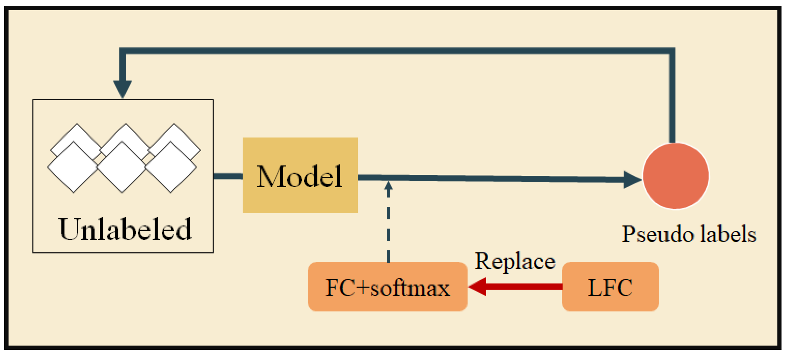
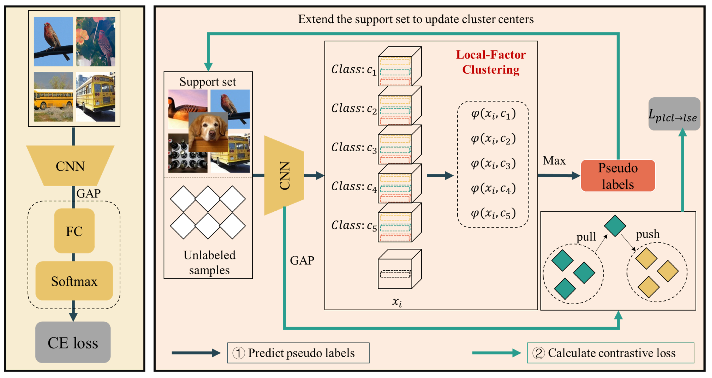
• We further propose a local factor clustering module to better acquire accurate pseudo-labels, which combines the local feature information of labeled and unlabeled samples.
• A series of experiments and analyses are conducted to demonstrate the progressiveness and robustness of our approach on two datasets.

Table 1. This paper presents explanations of abbreviations to better understand the paper description.

Number	Acronyms	Descriptions
1	FSL	few-shot learning
2	SSFSL	semi-supervised few-shot learning
3	UCL	the unsupervised contrastive learning module
4	PLCL	the pseudo-labeling guided contrastive learning module
5	LFC	the local factor clustering strategy
6	MFC	the multi-factor clustering strategy from [12]
7	KC	the kmeans clustering strategy from [9]
8	CE loss	cross-entropy loss
9	GAP	global average pooling operation

Table 1. This paper presents explanations of abbreviations to better understand the paper description.

Number	Acronyms	Descriptions
1	FSL	few-shot learning
2	SSFSL	semi-supervised few-shot learning
3	UCL	the unsupervised contrastive learning module
4	PLCL	the pseudo-labeling guided contrastive learning module
5	LFC	the local factor clustering strategy
6	MFC	the multi-factor clustering strategy from [12]
7	KC	the kmeans clustering strategy from [9]
8	CE loss	cross-entropy loss
9	GAP	global average pooling operation

2. Related Work

This section first briefly introduces the background of FSL and SSFSL, and then explores contrastive learning research.

2.1. Few-Shot Learning and Semi-Supervised Few-Shot Learning

In FSL, meta-learning-based methods and transfer learning-based methods are two broad categories of existing research. There are two main types of meta-learning-based studies: metrics-based [3,14] and optimization-based [4,15,16]. The former aims to learn good feature embeddings using the episodic training, where good feature embeddings mean that samples of the same class are close to each other, while samples of different classes are far from each other. While the latter tends to learn good and potential parameters to quickly adapt the model to the novel dataset. Most recently, the FSL method based on transfer learning achieves better performance compared to the FSL method based on meta-learning [6,8], and usually uses unlabeled samples from the novel dataset to learn the novel dataset’s embeddings rather than base dataset’s embeddings. To leverage unlabeled samples from the novel dataset is called semi-supervised few-shot learning, numerous methods [6,8,9,12,17,18,19] regarding SSFSL have emerged. Ref. [9] has proposed a new clustering method using the prototypical networks. Ref. [20] and PTN [21] have leveraged graph-based methods to improve the ability to predict labels. Cluster-FSL [12] has proposed a new clustering method: the multi-factor clustering to cluster.

Although these methods effectively improve the ability to obtain pseudo-labels, they ignore the impact of the local feature information. Therefore, in this paper, we propose the local factor clustering module to improve the promoting effect of contrastive learning on our model.

2.2. Contrastive Learning

Contrastive learning has received strong attention in recent years. InstDisc [22] has used a memory bank to reserve the embeddings of samples. Following this work, MoCo [21] has employed the queue to store the embeddings of samples and uses the momentum encoder to update the negative samples. SimCLR [23] has used a larger batch size to ensure sufficient negative samples and designed various data augmentations to complete unsupervised contrastive learning. However, the above methods are benefit instance discrimination [22], which does not conform to the classification at the class level. Therefore, inspired by [24], we focus on using pseudo-labeling to guide contrastive learning and obtain embeddings that are more suitable for the novel dataset in this paper.

3. Methodology

In this section, a problem definition on SSFSL is given, and then how to learn the base dataset’s embeddings is presented. Finally, the effect of the contrastive model with the local factor clustering strategy is emphasized. We present the important symbols used in the paper and their specific descriptions in

Table 2. This paper presents main symbols and descriptions to better understand the paper.

Number	Symbols	Descriptions
1	$D_{base},D_{novel}$	the base dataset and the novel dataset
2	$\mathcal{S},\mathcal{Q},\mathcal{U}$	the original support set, the query set and the unlabeled dataset
3	N	the number of categories in $D_{novel}$
4	$K,Q,R$	the number of labeled, tested, and unlabeled samples per category
5	$x_m^i,c_m^j,x_a^i,c_t^j$	the local feature descriptors for samples $x_i$ and class $c_j$
6	$\widehat{\mathcal{S}}$	the expanded support set with unlabeled samples
7	$ag{u}_1,au{g}_2$	two different data augmentations
8	$z_i^1,z_i^2,z_w,z_b,z_i$	feature embeddings after convolutional neural network
9	$B,W$	the number of positive and negative sample pairs
10	$f_{\theta }(·)$	convolutional neural network with parameter $\theta$
11	${\theta }^{{}^{\prime }}$	network parameters obtained after training on the base dataset
12	${\theta }^{*}$	network parameters obtained after training with the PLCL module

.

3.1. Problem Formulation

For N-way K-shot image classification, we randomly sample N classes and randomly sample K samples under each class as labeled samples. And a FSL task contains the support set and the query set. The support set is defined as $\mathcal{S}={\left\{(x_i,y_i)\right\}}_{i=1}^{N\times K}$ that has a few labeled samples, where $x_i$ is an image, $y_i$ is the label of $x_i$, and the query set is defined as $\mathcal{Q}={\left\{\left(x_i\right)\right\}}_{i=1}^{N\times Q}$, where Q is the number of images in each class, so the query set contains $N\times Q$ unlabeled samples for testing. Finally, the novel dataset is denoted as $D_{novel}=\mathcal{S}\cup \mathcal{Q}$. Most studies have introduced an auxiliary dataset $D_{base}$ to assist few-shot learning. Note that the classes in $D_{base}$ and $D_{novel}$ are different, formalized as $C_{base}\cap C_{novel}=\varnothing$. For SSFSL, we also have an extra unlabeled dataset $\mathcal{U}={\left\{\left(x_i\right)\right\}}_{i=1}^{N\times R}$ in the novel dataset, where R is the number of unlabeled samples for each class. Therefore, the novel dataset is defined as $D_{novel}=\mathcal{S}\cup \mathcal{Q}\cup \mathcal{U}$. With the help of a few samples from $\mathcal{S}$ and unlabeled samples from $\mathcal{U}$, we aim to correctly classify the samples from the query set.

The overall framework of our model with the LFC strategy and the PLCL module is shown in Figure 2, which mainly consists of two steps: (1) pre-training feature embeddings using the CE loss in $D_{base}$, and migrating the pre-trained embeddings to $D_{novel}$; (2) fine-tuning the pre-trained embeddings using the PLCL and LFC modules.

3.2. Pre-Training Feature Embeddings

The pre-training stage is shown on the left part of Figure 2, a deep network $f_{\theta }(·)$ is pre-trained in the base dataset and then transferred to the novel dataset. The use of prior knowledge for learning is very in line with human cognitive laws. Concretely, we start by pre-training $f_{\theta }(·)$ in the base dataset using $L_{ce}$:

$${\theta }^{{}^{\prime }}=\underset{\theta }{argmin}{L}_{ce}(D_{base};\theta ),$$

(1)

where $L_{ce}$ is the standard CE loss between the predicted labels and real labels as well as ${\theta }^{{}^{\prime }}$ is the most appropriate network parameter for the base dataset, but it may not necessarily be applicable to the novel dataset because the data distribution between the novel dataset and the base dataset is different. Therefore, we use the LFC strategy and the PLCL module to adjust this parameter next.

3.3. Fine-Tuning Feature Embeddings Using LFC and PLCL

To the best of our knowledge, the local feature information is considered in the following two scenarios [25,26,27]. (1) The known global information is extremely scarce. Few-shot learning usually pools the final feature map to obtain global representations, which ignores a lot of irretrievable local feature information. (2) Overemphasizing the feature information of the image background. The research related to the local feature information in FSL is as follows: DN4 [26] has proposed an image-to-class module that emphasizes that local information can greatly improve the FSL classification. InfoPatch [27] has learned that the stronger base dataset’s embeddings can eliminate data bias. Motivated by DN4 [26], we assume that local features can reflect more information during clustering compared to global features.

3.3.1. The Local Factor Clustering Module

Taking ResNet-12 as example, ResNet-12 is composed of four residual blocks, and the output dimensions of each residual block is [64,42,42], [128,21,21], [256,10,10] and [512,5,5]. And global feature representations with 512-dimension are obtained through the final global average pooling (GAP). Given an unlabeled sample $x_i$, the local feature set $f_{\theta }\left(x_i\right)=[x_1^i,x_2^i,...,x_m^i]\in {\mathbb{R}}^{d\times m}$ can be expressed, where $f_{\theta }(·)$ is ResNet-12 that removes the last global average pooling layer and $m=5\times 5=25$ and $d=512$. For the support set, we can obtain N clustering centers as follows:

$$c_j=\frac{1}{K}\sum _{i=1}^K{f}_{\theta }\left(x_i\right),j=1,2,...,N,$$

(2)

where similar to $x_i$, the local feature set in each center $c_j=[c_1^j,c_2^j,...,c_m^j]\in {\mathbb{R}}^{d\times m}$. For each local feature $x_a^i\in f_{\theta }\left(x_i\right)$, its k-nearest neighbors $c_t^j$ in each center $c_j$ are found, where $t=1,2,...,k$. Then, the similarity between $x_i$ and the clustering center $c_j$ is attained by calculating the similarity between $x_a^i$ and each $c_t^j$. This process is represented as follows:

$$\phi (x_i,c_j)=\sum _{a=1}^m\sum _{t=1}^{k}cos(x_a^i,c_t^j),$$

(3)

where $cos(,)$ indicates the cosine similarity. The pseudo-label of $x_i$ is $y_i^j=argmax\left\{\phi (x_i,c_j)\right\}$ and clustering center $c_j$ is updated with $x_i$. Finally, the clustering center set is represented as $[{\widehat{c}}_1,{\widehat{c}}_2,...,{\widehat{c}}_N]$. The final clustering result is regarded as obtaining pseudo-labels for unlabeled samples like this $\widehat{y_i}=argmax\left\{\phi (x_i,{\widehat{c}}_j)\right\}$. Thus, a dataset with pseudo-labeled samples is generated $\widehat{\mathcal{S}}=\mathcal{S}\cup \mathcal{U}$.

3.3.2. The Pseudo-Labeling Guided Contrastive Learning Module

In this section, we use the dataset $\widehat{\mathcal{S}}$ to implement the PLCL module. For conventional contrastive learning, the main approach is to construct supervised signals by performing different data augmentations on a sample to implicitly learn feature embeddings. Formally speaking, for a sample $x_i\in \widehat{\mathcal{S}}$, we can first apply two types of data augmentation operations to generate new samples $au{g}_1\left(x_i\right)$ and $au{g}_2\left(x_i\right)$ and then obtain its corresponding representations $z_i^1=GAP\left(f_{\theta }\left(au{g}_1\left(x_i\right)\right)\right)\in {\mathbb{R}}^d$ and $z_i^2=GAP\left(f_{\theta }\left(au{g}_2\left(x_i\right)\right)\right)\in {\mathbb{R}}^d$, where $d=512$. Usually, we use InfoNCE loss to represent contrastive learning by:

$$L_{ucl}=-log\frac{exp(cos(z_i^1,z_i^2)\gamma )}{exp(cos(z_i^1,z_i^2)\gamma )+{\sum }_{w=1}^{W}exp(cos(z_i^1,z_w)\gamma )},$$

(4)

where $\gamma$ denotes the temperature parameter as well as $cos(,)$ is the cosine similarity. W is the number of negative samples. Differentiating from $L_{ucl}$, there are two differences in pseudo-labeling guided contrastive learning. First, the designed loss requires us to complete clustering at the class level in the feature space. Second, LogSumExp loss instead of InfoNCE loss is used under multiple positive sample pairs. Here, we first use InfoNCE loss to express our loss function by

$$L_{plcl}=-log\frac{{\sum }_{b=1}^{B}exp(cos(z_i,z_b)\gamma )}{{\sum }_{b=1}^{B}exp(cos(z_i,z_b)\gamma )+{\sum }_{w=1}^{W}exp(cos(z_i,z_w)\gamma )},$$

(5)

where $z_i$ and $z_b$ have the same label, while $z_i$ and $z_w$ are not of the same class. B and W refer to the amount of positive and negative samples, respectively.

Analysis of Loss Function: To better illustrate that our loss function is feasible, we take the number of negative samples as the starting point for in-depth analysis of it. Unsupervised contrastive loss is implemented on the CE loss in deep learning platforms such as Tensorflow and PyTorch, UCL benefits from the quality of positive samples and the number of negative samples. Why do we need a large number of negative samples support in UCL? A conclusion drawn in FlatNCE [28] is that a small number of negative samples can lead to low-precision floating-point arithmetic. By using logarithmic operation rule: $-log\left(\frac{x}{x+y}\right)=log(1+\frac{y}{x})$, $L_{ucl}$ is rewritten as

$$L_{ucl}=log(1+\frac{{\sum }_{w=1}^{W}exp(cos(z_i^1,z_w)\gamma )}{exp(cos(z_i^1,z_i^2)\gamma )}),$$

(6)

where, if W is very low, $ϵ={\sum }_{w=1}^W[exp(cos(z_i^1,z_w)\gamma -cos(z_i^1,z_i^2)\gamma )]\to 0$ because $z_i^1$ and $z_i^2$ are obtained through different data augmentations on the same sample, i.e., $cos(z_i^1,z_i^2)\gg cos(z_i^1,z_w)$. The calculation of $ϵ$ inherently has floating-point errors, which result in the model not being able to provide effective gradients. Furthermore, the most direct way to alleviate this problem is to magnify $ϵ$ using a constant $C={ϵ}_{no\_gradient}$, thus we can reconstruct $L_{ucl}$ based on approximate Equation (7).

$$\left\{\begin{array}{c}\hfill log(1+x)\approx x\\ \hfill \nabla \frac{x}{x_{no\_gradient}}=\frac{\nabla x}{x_{no\_gradient}}=\frac{1}{x_{no\_gradient}}\\ \hfill \nabla logx=\frac{1}{x_{no\_gradient}}\end{array}\right.$$

(7)

$$L_{ucl\to lse}=log\sum _{w=1}^{W}exp(cos(z_i^1,z_w)\gamma )-logexp(cos(z_i^1,z_i^2)\gamma )$$

(8)

By Equation (8), the gradient of it is

$$\nabla L_{ucl\to lse}=\left\{\begin{array}{ccc}\frac{exp(cos(z_i,z_w)\gamma )}{{\sum }_{w=1}^{W}exp(cos(z_i,z_w)\gamma )}& & ifi\ne w\hfill \\ -1& & otherwise\hfill \end{array}\right..$$

(9)

By Equation (9), we can see that the network parameters can be updated normally in the case of a pair of positive samples. Similar to Equation (8), $p_{plcl}$ is rewritten as

$$L_{plcl\to lse}=log\sum _{w=1}^{W}exp(cos(z_i,z_w)\gamma )-log\sum _{b=1}^{B}exp(cos(z_i,z_b)\gamma ).$$

(10)

By Equation (10), the gradient of it is

$$\nabla L_{plcl\to lse}=\left\{\begin{array}{ccc}\hfill -\frac{exp(cos(z_i,z_b)\gamma )}{{\sum }_{b=1}^{B}exp(cos(z_i,z_b)\gamma )}& & ifi=b\hfill \\ \\ \hfill \frac{exp(cos(z_i,z_w)\gamma )}{{\sum }_{k=1}^{W}exp(cos(z_i,z_w)\gamma )}& & otherwise\hfill \end{array}\right..$$

(11)

By Equation (11), we can see that the network parameters can be updated normally in the case of multiple pair of positive samples.

3.4. Testing Using LFC and Feature Embeddings

In the PLCL module, we update the network parameters using $L_{plcl\to lse}$ and ultimately obtain the parameter ${\theta }^{*}$ from ${\theta }^{{}^{\prime }}$ to predict the labels of the samples from $\mathcal{Q}$ by prototypical networks. Each class prototypes is calculated by the mean embedding of samples with the same label:

$$p_j=\sum _{{\mathbb{I}}_{i=j}}GAP\left(f_{{\theta }^{*}}\left(x_i\right)\right),$$

(12)

where $\mathbb{I}$ is a conditional indicator function, representing whether $x_i$ belongs to the class prototype $p_j$, then the class prototype is updated with $f_{{\theta }^{*}}\left(x_i\right)$. The classes of samples in query set $\mathcal{Q}$ are obtained by $y_i=argmax\{cos(q_i,p_j)\}$, where $cos(,)$ indicates the cosine similarity and $q_i$ is an image from $\mathcal{Q}$.

4. Experiment

In the experimental section, we perform our experiments on two datasets: mini-ImageNet [3] and tiered-ImageNet [9]. Also, we further conduct other experiments to demonstrate the progressiveness and robustness of our model. In the evaluation, we sample $N=5$, $K=1$ or 5 and $Q=15$ to test the performance of FSL. We repeat the test experiments 600 times and report the mean accuracy together with a corresponding 95% confidence interval.

4.1. Datasets

The number of categories and samples for the training, validation, and testing sets in the mini-ImageNet and tiered-ImageNet datasets are summarized in

Table 3. The training set, validation set, and test set for mini-ImageNet and tiered-ImageNet datasets, including number of categories and images.

		Train	Val	Test
mini-ImageNet	Classes	64	16	20
	Images	38,400	9600	12,000
tiered-ImageNet	Classes	351	97	160
	Images	448,695	124,261	206,209

.

4.1.1. Mini-ImageNet

The mini-ImageNet dataset is a frequently-used dataset for FSL classification and is the subset of ImageNet, containing 60,000 samples from 100 classes. In general, we divided this dataset into 64 classes as training set, 16 classes as validation set, and 20 classes as test set. All images are of size 84 × 84.

4.1.2. Tiered-ImageNet

The tiered-ImageNet dataset contains 608 classes that is composed of 34 super-classes. Overall, 34 super-classes are split into 20 super-classes (351 sub-classes) containing 448,695 samples as training set, 6 super-classes (97 sub-classes) containing 124,261 samples as validation set and 8 super-classes (160 sub-classes) containing 206,209 samples as test set. This dataset aims to minimize the semantic similarity between the splits. And it is a larger subset of ImageNet than mini-ImageNet. All images are of size 84 × 84.

4.2. Implementation Details

At the pre-training stage, we use the ResNet-12 as the backbone. For optimization, the model uses SGD with a momentum of 0.9, a weight decay of 0.0005, the learning rate is initially set to 1, and then changed to 0.1, 0.01, and 0.001 at epochs 60, 80 and 90, respectively. The batch size is set to 128 and the base model is trained for 100 epochs. Note that in the base dataset, we only used 64 classes for training instead of 80 classes. At the fine-tuning stage, the base model is transferred to the novel dataset and then is fine-tuned on both a few labeled samples and substantial unlabeled samples. We set weight decay to 0.0005, learning rate to 0.001, and use the SGD optimizer with a momentum of 0.9. In addition, we also set the hyper-parameters as follows, the temperature parameter $\lambda =1$ in the PLCL module, the quantity of unlabeled samples per category $R=[0,30,50,100]$ and the number of nearest neighbors $k=[1,3,5,7]$ to calculate the similarity between the samples and the clustering centers in the LFC strategy. In the following experiments, we check the optimal settings of these hyper-parameters in detail.

4.3. Experimental Results

This section mainly reports our experimental results compared to the advanced methods and conducts experiments under different settings.

4.3.1. Comparison with Advanced Methods

We report our experimental results from two aspects: (1) in terms of FSL approaches, and (2) in terms of SSFSL approaches. Here, to ensure fairness in comparison, we use two settings, namely 30/50 and 100/100, where the first number (30 or 100) refers to one-shot and the second (50 or 100) to five-shot. For mini-ImageNet, from

Table 4. Classification accuracy (%) comparison with the state-of-the-art methods for five-way classification on mini-ImageNet and tiered-ImageNet. † represents the used semi-supervised setting is (30/50). The best-performing result is bold.

Methods	Backbone	mini-ImageNet		tiered-ImageNet
		5-Way 1-Shot	5-Way 5-Shot	5-Way 1-Shot	5-Way 5-Shot
MatchingNet [3]	ConvNet-64	43.56 ± 0.84	55.31 ± 0.73	-	-
ProtoNet [13]	ConvNet-64	49.42 ± 0.78	68.20 ± 0.66	53.31 ± 0.89	72.69 ± 0.74
MAML [4]	ConvNet-64	48.70 ± 1.84	63.11 ± 0.92	51.67 ± 1.81	70.30 ± 1.75
DN4 [26]	ConvNet-64	51.24 ± 0.74	71.02 ± 0.64	-	-
RFS [29]	ResNet-12	64.80 ± 0.60	82.14 ± 0.43	71.52 ± 0.69	86.03 ± 0.49
TADAM [30]	ResNet-12	58.50 ± 0.30	76.70 ± 0.30	-	-
RENet [31]	ResNet-12	67.60 ± 0.44	82.58 ± 0.30	71.61 ± 0.51	85.28 ± 0.35
SetFeat [32]	ResNet-12	68.32 ± 0.62	82.71 ± 0.41	68.32 ± 0.62	82.71 ± 0.41
FRN [33]	ResNet-12	66.45 ± 0.19	82.83 ± 0.13	71.16 ± 0.22	86.01 ± 0.15
infoPatch [27]	ResNet-12	67.67 ± 0.45	82.44 ± 0.31	71.51 ± 0.52	85.44 ± 0.35
MetaOptNet [16]	ResNet-12	64.09 ± 0.62	80.00 ± 0.45	65.99 ± 0.72	81.56 ± 0.53
TPN-semi [20]	ConvNet-64	52.78 ± 0.27	66.42 ± 0.21	55.74 ± 0.29	71.01 ± 0.23
Mask soft k-means [9]	WRN-28-10	52.35 ± 0.89	67.67 ± 0.65	52.39 ± 0.44	69.88 ± 0.20
TransMatch [6]	WRN-28-10	62.93 ± 1.11	81.19 ± 0.59	72.19 ± 1.27	82.12 ± 0.92
LST ${}^{†}$ [10]	ResNet-12	70.10 ± 1.90	78.70 ± 0.80	77.70 ± 1.60	85.20 ± 0.80
LR + ICI ${}^{†}$ [34]	ResNet-12	67.57 ± 0.97	79.07 ± 0.56	83.32 ± 0.87	89.06 ± 0.51
iLPC ${}^{†}$ [35]	ResNet-12	70.99 ± 0.91	81.06 ± 0.49	85.04 ± 0.79	89.63 ± 0.47
Ours ${}^{†}$ ($k=3$)	ResNet-12	71.66 ± 1.04	82.57 ± 0.56	86.07 ± 0.69	89.07 ± 0.01
Ours ($k=3$)	ResNet-12	74.46 ± 1.21	83.21 ± 0.57	87.06 ± 0.91	90.21 ± 0.57

, it can be concluded that our method has improved by 6.14% and 0.38% for one-shot and five-shot (SetFeat, FRN). Under the 100/100 setting, our method has improved by 11.53% and 2.02% for one-shot and five-shot (TransMatch). Under the 30/50 setting, our method has improved by 0.67% and 1.51% for one-shot and five-shot (iLPC). For tiered-ImageNet, our method has also achieved very competitive results. All the above results demonstrate the significance of our method.

4.3.2. The Impact of Unlabeled Samples

Table 5. Classification accuracy (%) with different quantities of unlabeled samples per class on mini-ImageNet. The best performance is bold.

R=	5-Way 1-Shot	5-Way 5-Shot
0	52.24 ± 0.81	72.32 ± 0.65
30	71.66 ± 1.04	81.20 ± 0.55
50	72.80 ± 1.09	82.57 ± 0.56
100	74.46 ± 1.21	83.21 ± 0.57

shows the experimental results under different numbers of unlabeled samples. In our method, the use of unlabeled samples is crucial, especially as the initial labeled samples are very few. We found that more unlabeled samples have a very significant effect on improving performance under the setting of unlabeled samples $R=[0,30,50,100]$, which also inspires us to strengthen the additional information brought by mining unlabeled samples, especially in few-shot learning, where only a few samples are available.

4.3.3. The Impact of Nearest Neighbors

When conducting the LFC strategy, we use the k-nearest neighbor to measure the similarities between samples and clustering centers.

Table 6. Classification accuracy (%) with different quantities of nearest neighbors k on mini-ImageNet. The best performance is bold.

k=	5-Way 1-Shot	5-Way 5-Shot
1	74.50 ± 1.20	83.26 ± 0.59
3	74.46 ± 1.21	83.21 ± 0.57
5	74.43 ± 1.21	83.30 ± 0.56
7	74.35 ± 1.19	83.18 ± 0.57

shows the changes in the performance of our method under different quantities of nearest neighbors. The number of k does indeed effect the overall performance of our model, but the overall difference is not significant.

4.4. Ablation Study

We conducted ablation studies on our method to illustrate the influence of the PLCL module and the LFC strategy on the model performance.

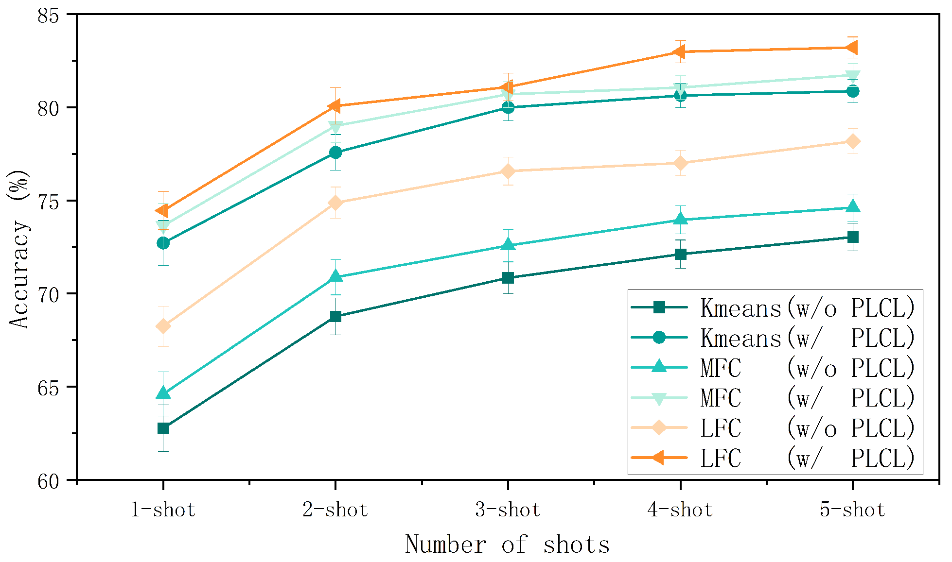
4.4.1. The Influence of PLCL

The following conclusions can be drawn from Figure 3. (1) Regardless of the method used to obtain pseudo-labels, the PLCL module is essential and can significantly improve model performance; (2) the higher the accuracy of obtaining pseudo-labels, coupled with the higher model performance of the PLCL module.

Table 7. Classification accuracy (%) with UCL or PLCL on mini-ImageNet. The best performance is bold. ↑ is an increase in classification accuracy.

Method	5-Way 1-Shot	5-Way 5-Shot
MFC + UCL	73.55 ± 1.19	81.64 ± 0.61
MFC + PLCL	73.65 ± 1.19 (↑ 0.10)	81.77 ± 0.61 (↑ 0.13)
LFC + UCL	74.33 ± 1.21	83.00 ± 0.57
LFC + PLCL	74.46 ± 1.21 (↑ 0.13)	83.21 ± 0.57 (↑ 0.21)

shows the changes in model performance under both UCL and PLCL. Although the PLCL module can raise the accuracy of FSL, it does not change much. However, we can know that the more correct the pseudo-labels are, the more effective our method is compared with UCL.

4.4.2. The Influence of LFC

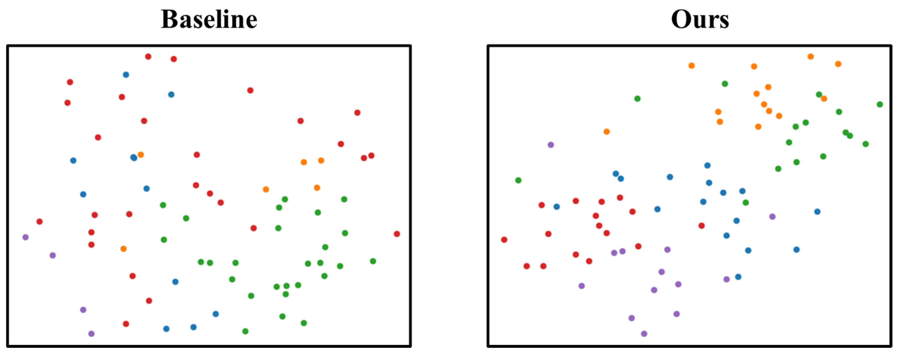
Compared to conventional clustering methods [9,12], our method prefers the local feature information.

Table 8. The impact of different methods of obtaining pseudo-labels. The best performance is bold.

Method	5-Way 1-Shot	5-Way 5-Shot
KC [9]	62.79 ± 1.25%	73.04 ± 0.74%
MFC [12]	64.62 ± 1.18%	74.62 ± 0.73%
LFC	68.25 ± 1.18%	78.18 ± 0.67%
KC + PLCL	72.72 ± 1.21%	80.87 ± 0.63%
MFC + PLCL	73.65 ± 1.19%	81.77 ± 0.61%
LFC + PLCL (Ours)	74.46 ± 1.21%	83.21 ± 0.57%

and Figure 3 summarize the performance impact of LFC on the model with PLCL and without PLCL. Without PLCL, LFC has improved by 3.63% and 3.56% for one-shot and five-shot compared to MFC. With PLCL, LFC has improved by 0.81% and 1.44% for one-shot and five-shot compared to MFC. These results indicate that LFC can obtain more accurate pseudo-labeled samples, and play a promoting role in the PLCL module, which inspires us to focus more research on how to obtain higher quality pseudo-labels.

4.5. Visualization

The availability of our method is evident. In this section, we explore the mechanisms for improvement through visualization. The t-SNE is used to visualize the embeddings. Specifically, we sample an episode from the novel dataset of mini-ImageNet, and an episode contains 75 test samples which are input into the model to obtain embeddings as shown in Figure 4, whose result states that our method generate more compact clusters than baseline, where baseline refers to directly using the base dataset’s embeddings in the novel dataset without any other operations. That is to say, the network parameters used on the left are ${\theta }^{{}^{\prime }}$, while the network parameters used on the right are ${\theta }^{*}$, which are obtained by the PLCL module.

5. Conclusions

We propose a contrastive model with the local factor clustering strategy for SSFSL to effectively alleviate the embeddings mismatch problem due to the objective discrepancy that the underlying base dataset’s class distribution is different from novel dataset’s class distribution. Specifically, we first pre-train feature embeddings in the base dataset, and then transfer the pre-trained embeddings to the novel dataset for training. During the fine-tuning process, we first use the local factor clustering strategy to enhance the accuracy of pseudo-labels, and then pseudo-labeling guided contrastive learning is achieved on these unlabeled samples. Finally, LFC and a prototypical classifier are utilized to test, where LFC is a novel clustering method that reflects on the local feature information of labeled and unlabeled samples. On the two benchmark datasets, our method exceeds many FSL and SSFSL methods. Ablation experiments and visualization have also been performed to further validate the progressiveness of our approach.

References

1. Fei-Fei, L.; Fergus, R.; Perona, P. One-shot learning of object categories. IEEE Trans. Pattern Anal. Mach. Intell. 2006, 28, 594–611. [Google Scholar] [CrossRef] [PubMed] [Green Version]
2. Wang, Y.; Yao, Q.; Kwok, J.T.; Ni, L.M. Generalizing from a few examples: A survey on few-shot learning. ACM Comput. Surv. (CSUR) 2020, 53, 1–34. [Google Scholar] [CrossRef]
3. Vinyals, O.; Blundell, C.; Lillicrap, T.; Wierstra, D. Matching networks for one shot learning. Adv. Neural Inf. Process. Syst. 2016, 29, 3637–3645. [Google Scholar]
4. Finn, C.; Abbeel, P.; Levine, S. Model-agnostic meta-learning for fast adaptation of deep networks. In Proceedings of the International Conference on Machine Learning, PMLR, Fort Lauderdale, FL, USA, 20–22 April 2017; pp. 1126–1135. [Google Scholar]
5. Dhillon, G.S.; Chaudhari, P.; Ravichandran, A.; Soatto, S. A baseline for few-shot image classification. In Proceedings of the International Conference on Learning Representations, Addis Ababa, Ethiopia, 26–30 April 2020. [Google Scholar]
6. Yu, Z.; Chen, L.; Cheng, Z.; Luo, J. Transmatch: A transfer-learning scheme for semi-supervised few-shot learning. In Proceedings of the IEEE/CVF Conference on Computer Vision and Pattern Recognition, Seattle, WA, USA, 13–19 June 2020; pp. 12856–12864. [Google Scholar]
7. Chen, W.Y.; Liu, Y.C.; Kira, Z.; Wang, Y.C.; Huang, J.B. A Closer Look at Few-shot Classification. In Proceedings of the International Conference on Learning Representations, New Orleans, LA, USA, 6–9 May 2019. [Google Scholar]
8. Huang, H.; Zhang, J.; Zhang, J.; Wu, Q.; Xu, C. Ptn: A poisson transfer network for semi-supervised few-shot learning. In Proceedings of the AAAI Conference on Artificial Intelligence, New York, NY, USA, 19–21 May 2021; Volume 35, pp. 1602–1609. [Google Scholar]
9. Ren, M.; Triantafillou, E.; Ravi, S.; Snell, J.; Swersky, K.; Tenenbaum, J.B.; Larochelle, H.; Zemel, R.S. Meta-learning for semi-supervised few-shot classification. In Proceedings of the 6th International Conference on Learning Representations ICLR, Vancouver, BC, Canada, 30 April–3 May 2018. [Google Scholar]
10. Li, X.; Sun, Q.; Liu, Y.; Zhou, Q.; Zheng, S.; Chua, T.S.; Schiele, B. Learning to self-train for semi-supervised few-shot classification. Adv. Neural Inf. Process. Syst. 2019, 32, 10276–10286. [Google Scholar]
11. Huang, K.; Geng, J.; Jiang, W.; Deng, X.; Xu, Z. Pseudo-loss confidence metric for semi-supervised few-shot learning. In Proceedings of the IEEE/CVF International Conference on Computer Vision, Montreal, BC, Canada, 10–17 October 2021; pp. 8671–8680. [Google Scholar]
12. Ling, J.; Liao, L.; Yang, M.; Shuai, J. Semi-Supervised Few-shot Learning via Multi-Factor Clustering. In Proceedings of the 2022 IEEE/CVF Conference on Computer Vision and Pattern Recognition (CVPR), New Orleans, LA, USA, 18–24 June 2022; pp. 14544–14553. [Google Scholar]
13. Snell, J.; Swersky, K.; Zemel, R. Prototypical networks for few-shot learning. Adv. Neural Inf. Process. Syst. 2017, 30, 4080–4090. [Google Scholar]
14. Zhang, J.; Zhao, C.; Ni, B.; Xu, M.; Yang, X. Variational Few-Shot Learning. In Proceedings of the 2019 IEEE/CVF International Conference on Computer Vision (ICCV), Seoul, Republic of Korea, 27 October–2 November 2019; pp. 1685–1694. [Google Scholar]
15. Fallah, A.; Mokhtari, A.; Ozdaglar, A. On the convergence theory of gradient-based model-agnostic meta-learning algorithms. In Proceedings of the International Conference on Artificial Intelligence and Statistics, PMLR, Online, 26–28 August 2020; pp. 1082–1092. [Google Scholar]
16. Lee, K.; Maji, S.; Ravichandran, A.; Soatto, S. Meta-Learning with Differentiable Convex Optimization. In Proceedings of the 2019 IEEE/CVF Conference on Computer Vision and Pattern Recognition (CVPR), Long Beach, CA, USA, 15–20 June 2019; pp. 10649–10657. [Google Scholar]
17. Yang, Z.; Wang, J.; Zhu, Y. Few-shot classification with contrastive learning. In Proceedings of the Computer Vision–ECCV 2022: 17th European Conference, Tel Aviv, Israel, 23–27 October 2022; Proceedings, Part XX. Springer: Berlin/Heidelberg, Germany, 2022; pp. 293–309. [Google Scholar]
18. Wei, X.S.; Xu, H.Y.; Zhang, F.; Peng, Y.; Zhou, W. An Embarrassingly Simple Approach to Semi-Supervised Few-Shot Learning. Adv. Neural Inf. Process. Syst. 2022, 35, 14489–14500. [Google Scholar]
19. Hou, Z.; Kung, S.Y. Semi-Supervised Few-Shot Learning from A Dependency-Discriminant Perspective. In Proceedings of the IEEE/CVF Conference on Computer Vision and Pattern Recognition, New Orleans, LA, USA, 18–24 June2022; pp. 2817–2825. [Google Scholar]
20. Liu, Y.; Lee, J.; Park, M.; Kim, S.; Yang, E.; Hwang, S.J.; Yang, Y. Learning to propagate labels: Transductive propagation network for few-shot learning. arXiv 2018, arXiv:1805.10002. [Google Scholar]
21. He, K.; Fan, H.; Wu, Y.; Xie, S.; Girshick, R. Momentum contrast for unsupervised visual representation learning. In Proceedings of the IEEE/CVF Conference on Computer Vision and Pattern Recognition, Seattle, WA, USA, 14–19 June 2020; pp. 9729–9738. [Google Scholar]
22. Wu, Z.; Xiong, Y.; Yu, S.X.; Lin, D. Unsupervised feature learning via non-parametric instance discrimination. In Proceedings of the IEEE Conference on Computer Vision and Pattern Recognition, Salt Lake City, UT, USA, 18–23 June 2018; pp. 3733–3742. [Google Scholar]
23. Chen, T.; Kornblith, S.; Norouzi, M.; Hinton, G. A simple framework for contrastive learning of visual representations. In Proceedings of the International Conference on Machine Learning, PMLR, Virtual, 13–18 July 2020; pp. 1597–1607. [Google Scholar]
24. Khosla, P.; Teterwak, P.; Wang, C.; Sarna, A.; Tian, Y.; Isola, P.; Maschinot, A.; Liu, C.; Krishnan, D. Supervised contrastive learning. Adv. Neural Inf. Process. Syst. 2020, 33, 18661–18673. [Google Scholar]
25. Ouali, Y.; Hudelot, C.; Tami, M. Spatial contrastive learning for few-shot classification. In Proceedings of the Machine Learning and Knowledge Discovery in Databases, Research Track: European Conference, ECML PKDD 2021, Bilbao, Spain, 13–17 September 2021; Proceedings, Part I 21. Springer: Berlin/Heidelberg, Germany, 2021; pp. 671–686. [Google Scholar]
26. Li, W.; Wang, L.; Xu, J.; Huo, J.; Gao, Y.; Luo, J. Revisiting local descriptor based image-to-class measure for few-shot learning. In Proceedings of the IEEE/CVF Conference on Computer Vision and Pattern Recognition, Long Beach, CA, USA, 15–20 June 2019; pp. 7260–7268. [Google Scholar]
27. Liu, C.; Fu, Y.; Xu, C.; Yang, S.; Li, J.; Wang, C.; Zhang, L. Learning a few-shot embedding model with contrastive learning. In Proceedings of the AAAI Conference on Artificial Intelligence, New York, NY, USA, 19–21 May 2021; Volume 35, pp. 8635–8643. [Google Scholar]
28. Chen, J.; Gan, Z.; Li, X.; Guo, Q.; Chen, L.; Gao, S.; Chung, T.; Xu, Y.; Zeng, B.; Lu, W.; et al. Simpler, faster, stronger: Breaking the log-k curse on contrastive learners with flatnce. arXiv 2021, arXiv:2107.01152. [Google Scholar]
29. Tian, Y.; Wang, Y.; Krishnan, D.; Tenenbaum, J.B.; Isola, P. Rethinking few-shot image classification: A good embedding is all you need? In Proceedings of the Computer Vision–ECCV 2020: 16th European Conference, Glasgow, UK, 23–28 August 2020; Proceedings, Part XIV 16. Springer: Berlin/Heidelberg, Germany, 2020; pp. 266–282. [Google Scholar]
30. Oreshkin, B.; Rodríguez López, P.; Lacoste, A. TADAM: Task dependent adaptive metric for improved few-shot learning. In Proceedings of the Advances in Neural Information Processing Systems, Montréal, QC, Canada, 3–8 December 2018; Volume 31. [Google Scholar]
31. Kang, D.; Kwon, H.; Min, J.; Cho, M. Relational embedding for few-shot classification. In Proceedings of the IEEE/CVF International Conference on Computer Vision, Montreal, QC, Canada, 10–17 October 2021; pp. 8822–8833. [Google Scholar]
32. Li, Z.; Wang, L.; Ding, S.; Yang, X.; Li, X. Few-Shot Classification With Feature Reconstruction Bias. In Proceedings of the 2022 Asia-Pacific Signal and Information Processing Association Annual Summit and Conference (APSIPA ASC), Chiang Mai, Thailand, 7–10 November 2022; pp. 526–532. [Google Scholar]
33. Wertheimer, D.; Tang, L.; Hariharan, B. Few-shot classification with feature map reconstruction networks. In Proceedings of the IEEE/CVF Conference on Computer Vision and Pattern Recognition, Virtual, 19–25 June 2021; pp. 8012–8021. [Google Scholar]
34. Wang, Y.; Xu, C.; Liu, C.; Zhang, L.; Fu, Y. Instance Credibility Inference for Few-Shot Learning. In Proceedings of the 2020 IEEE/CVF Conference on Computer Vision and Pattern Recognition (CVPR), Seattle, WA, USA, 13–19 June 2020; pp. 12833–12842. [Google Scholar]
35. Lazarou, M.; Stathaki, T.; Avrithis, Y. Iterative label cleaning for transductive and semi-supervised few-shot learning. In Proceedings of the IEEE/CVF International Conference on Computer Vision, Montreal, BC, Canada, 10–17 October 2021; pp. 8751–8760. [Google Scholar]
Figure 1. Semi-supervised learning based on pseudo-labeling. The most common way to obtain pseudo-labels is to use a fully connected layer and a softmax function. In this paper, the LFC strategy has been proposed to replace this classifier.
Mathematics 11 03394 g001
Figure 2. Overall framework. We first pre-train feature embeddings in the base dataset using the standard CE loss. The pre-trained embeddings are then fine-tuned with unlabeled samples from the novel dataset by adopting the LFC and PLCL modules. For calculating contrastive loss, the same color blocks represent the same class of samples. Our goal is to make samples of the same class approach each other in the feature space, while samples of different labels stay away from each other.
Mathematics 11 03394 g002
Figure 3. The influence of pseudo-labeling guided contrastive learning. We report the experimental results of with (w/) PLCL and without (w/o) PLCL.
Mathematics 11 03394 g003
Figure 4. We visualize some samples from novel dataset by t-SNE. Dots of the same color represent that they belong to the same class.
Mathematics 11 03394 g004