Electrohydrodynamic Couette–Poiseuille Flow Instability of Two Viscous Conducting and Dielectric Fluid Layers Streaming through Brinkman Porous Medium

Abstract

The electrohydrodynamic plane Couette–Poiseuille flow instability of two superposed conducting and dielectric viscous incompressible fluids confined between two rigid horizontal planes under the action of a normal electric field and pressure gradient through Brinkman porous medium has been analytically investigated. The lower plane is stationary, while the upper one is moving with constant velocity. The details of the base state mathematical model and the linearized model equations for the perturbed state are introduced. Following the usual procedure of linear stability analysis for viscous fluids, we derived two non-dimensional modified Orr–Sommerfeld equations and obtained the associated boundary and interfacial conditions suitable for the problem. The eigenvalue problem has been solved using asymptotic analysis for wave numbers in the long-wavelength limit to obtain a very complicated novel dispersion relation for the wave velocity through lengthy calculations. The obtained dispersion equation has been solved using Mathematica software v12.1 to study graphically the effects of various parameters on the stability of the system. It is obvious from the figures that the system in the absence of a porous medium and/or electric field is more unstable than in their presence. It is found also that the velocity of the upper rigid boundary, medium permeability, and Reynolds number have dual roles on the stability on the system, stabilizing as well as destabilizing depending on the viscosity ratio value. The electric potential, dielectric constant and pressure gradient are found to have destabilizing influences on the system, while the porosity of the porous medium, density ratio and Froude number have stabilizing influences. A depth ratio of less than one has a dual role on the stability of the system, while it has a stabilizing influence for values greater than one. It is observed that the viscosity stratification brings about a stabilizing as well as a destabilizing effect on the flow system.

1. Introduction

Due to their occurrence in numerous applications, including simple oil–water two-phase flows, complex co-extrusion polymer melts, and the flow of cryolite/aluminum melts in a conventional Al reduction cell, the hydrodynamic instabilities of superposed fluid layers have attracted research interest over the years. The stability of the interface between the two fluids, which must be stable in order to guarantee the necessary mechanical, optical, and barrier properties of the products, is a significant challenge in this context. On the other hand, a very unstable interface has crucial uses in improved mass, momentum, and heat transmission, particularly in micro- and nanoscale devices. The viscosity and/or density stratification of the fluid layers, the thickness ratio of the layers’ jump in the velocities or the stresses across the interface, the properties of the fluids and the confining substrates, and other factors all affect how stable or unstable the interface is [1].

It is possible for liquid–gas or liquid–liquid flows with flat interfaces to exhibit zero-critical wave number instability with respect to disturbances of relatively long wavelength. The term “longwave” refers to this type of instability, which can be caused by a number of physical processes, such as the gravitational force’s longitudinal component [2,3], the variation in the liquid phase’s properties, such as viscosity [4,5,6,7,8,9], and the electric field [10,11,12]. The first research on the linear stability of two superposed fluids in a planar Poiseuille flow was published by Yih [4] who dveloped a general expression for the complex wave speed and offered an analysis for two-dimensional, long-wavelength perturbations. The interfacial mode’s growth rate is consequently influenced by the flow system’s geometrical and physical factors, notably the viscosity ratio m, the thickness ratio n, and density ratio r; nevertheless, he did not specifically address which of these factors affects the growth rate, and he gave numerical results only for the case $r=1$, $n=1$, providing that instability can be brought on by viscosity stratification alone. Yih did point out that a stabilizing density stratification $(r\ne 1)$ could outweigh the destabilizing effects of viscosity stratification. The effect of the thickness ratio n on the interfacial mode in plane Poiseuille flow was not discussed in his study. A detailed experimental examination for the flow stability of two superposed fluids flow was conducted by Kao and Park [13]. Their findings showed that if the Reynolds number exceeds a threshold value, the flow becomes unstable. In addition to the experimental study, the stability of stratified flow had been examined using a variety of theoretical and numerical methods; see refs. [14,15,16,17,18,19,20,21,22]. For an excellent review about the stability due to viscosity stratification, see the work of Govindarajan and Sahu [23].

Electrohydrodynamics (EHD) is a study of the flow field affected by an electric field that was first developed by Melcher and Taylor [24]. Electrohydrodynamics involves interactions between fluid motion and electric fields, and it studies the interplay of mechanical and electrical forces in fluids. Due to discontinuities in the electrical permittivities and conductivities of the fluids, if an electric field is present, the boundary between two fluids may become unstable [25]. EHD instabilities have been used for droplet generation purposes for immiscible fluids [26] or to enhance the rapid mixing of miscible fluids [27]. The surface-coupled or model for immiscible fluids assumes changes in the electrical characteristics of the fluids at the interface and the presence of electric forces exclusively under those situations [28,29,30,31,32]. On the basis of their electrical characteristics, the fluids can be categorized as perfect conductors [33] or perfect dielectric [34]. In a dielectric fluid that is flawless in every way, there is no free charge, and in one that is leaky, the conductivity profile is uniform. The electric field can be applied either parallel [35] or normal to the flat interface [36]. Li et al. [37] conducted theoretical and experimental research on the EHD instability of the interface between a conducting fluid and a dielectric fluid and came to the conclusion that the width of the channel, the total flow rate of the fluids, or the viscosity of the conducting fluid all affect the critical electric field. They [38] also looked at the electrohydrodynamic instability of an interface between two viscous fluids flowing in a microchannel under a normal electric field with different electrical properties analytically and experimentally. They came to the conclusion that the external electric field and growing microchannel width destabilize the interface between the immiscible fluids, whereas the viscosity of the high electrical mobility fluid has a stabilizing effect. For a recent excellent study about EHD instability between three immiscible fluids in a microchannel, see the paper of Eribol et al. [39].

On the other hand, over the past few decades, flows through porous media have attracted a lot of attention. There are a lot of engineering applications in different fields, such as geophysical, thermal and insulation engineering, modeling of packed sphere beds, cooling of electronic systems, groundwater hydrology, chemical catalytic reactors, ceramic processes, grain storage devices, fiber and granular insulation, petroleum reservoirs, coal combustors, ground water pollution, and filtration processes, to name just a few of these applications [40,41]. Much of the recent work on this topic is reviewed by Nield and Bejan [42] and Allen III et al. [43]. The majority of earlier investigations on porous media have considered Darcy’s law, and Forschheimer extended Darcy’s law as a recognized empirical formula that links the gravitational force, the bulk viscous resistance, and the pressure gradient in a porous material. In this instance, the resistive term $-(\mu /k_1)$$\mathbf{v}$ takes the place of the typical viscous term in the equation of motion, where $\mu$ is the fluid viscosity, $k_1$ is the medium permeability, and v is the Darcian velocity of the fluid. Despite their applications in many interesting disciplines, EHD stability studies for flows in porous medium have received little attention in the scientific literature; see the survey presented by Del Rio and Whitaker [44].

The goal of the current paper aims to explore the longwave stability analysis of two immiscible superposed conducting and dielectric fluids with limited depths between two rigid barriers. The lower boundary is stationary, while the upper boundary is moving at a constant speed $U_0$ under the effect of a normal electric field and the presence of a pressure gradient. To the best of our knowledge, this is the sole paper that focuses on the linear analysis of electrohydrodynamic instability in the longwave limit between conducting and dielectric fluids flowing in a channel with finite thicknesses through a porous medium. The current study extends Yiantsios and Higgins’ [14] analysis of the stability of a two-layer plane Poiseuille flow of two incompressible, immiscible viscous fluids separated by a surface tension interface to the case of Couette–Poiseuille flow for conducting and dielectric fluids in the presence of a transverse electric field through porous media.The obtained results can roughly be applied in pertinent applications, such as co-extruction applications where multi-layered items are necessary to manifest a steady interface to gain superior mechanical qualities.

The essay is structured as follows: Section 2 presents the specifics of the physical system and the mathematical model. The base state profiles and the linearized model equations for the perturbed state are provided in Section 3, while the derivations of two Orr–Sommerfeld equations are offered in Section 4. In Section 5, the associated boundary and interfacial conditions suitable for the problem are introduced. In Section 6, a very complex dispersion relation for the wave velocity is obtained by investigating the eigenvalue problem solutions using two-step approximations with very time-consuming calculations; and in Section 7, to investigate the influence of different parameters on the stability of the system, the derived dispersion equation has been solved using mathematica software v12.1. Section 8 includes the conclusions of the obtained findings in this study. Two lengthy functions that appear in the solutions of Orr–Sommerfeld equations are described in full in Appendix A at the end of the paper.

2. Mathematical Model and Dimensionless Equations

Consider two viscous, incompressible, streaming electrified fluids with finite depths flowing steadily in a gravitational field through a porous media of porosity $\epsilon$ and medium permeability $k_1$. It is known that the stability or instability of three-dimensional disturbances may be inferred from that of two-dimensional disturbances for the channel flow of homogeneous fluids between rigid limits as shown by Yih [4]. Therefore, it suffices to merely take the issue of two-dimensional disturbances into consideration here. In the Cartesian coordinate system, the coordinate axes are $X-Y$ with the origin at the interface between the two fluids; see Figure 1.

The upper fluid is of density ${\rho }^{\left(1\right)}$ and depth $d^{\left(1\right)}$, and we assume that it is a viscous conducting fluid whose fixed density and velocity components are provided by

$${\rho }_0^{\left(1\right)}={\rho }^{\left(1\right)}=\mathrm{canstant},u_0^{\left(1\right)}=u_0^{\left(1\right)}\left(Y\right)\mathrm{and}{v}_0^{\left(1\right)}=0,$$

where u and v are the velocity components in the directions of increasing X and Y, respectively. The upper fluid is bounded from above by a rigid boundary at $Y=d^{\left(1\right)}$ moving with constant velocity $U_0$. The lower fluid is of density ${\rho }^{\left(2\right)}$ and depth $d^{\left(2\right)}$, and the density and velocity components in the stationary state are assumed to be those of a viscous dielectric fluid, and they are given by

$${\rho }_0^{\left(2\right)}={\rho }^{\left(2\right)}=\mathrm{canstant},u_0^{\left(2\right)}=u_0^{\left(2\right)}\left(Y\right)\mathrm{and}{v}_0^{\left(2\right)}=0.$$

The lower fluid is bounded from below by a rigid conducting plane having electric potential ${\overline{V}}_0$ at $Y=-d^{\left(2\right)}$. In the stationary state, the interface between the two fluids is given by $Y=0$, the lower fluid is subject to a constant electric field ${\overline{\mathit{E}}}_0^{\left(2\right)}={\overline{E}}_0^{\left(2\right)}\mathit{j}$, and $\mathit{j}$ is the unit vector in the Y-direction. Also, the gravitational force $\mathit{g}=-g\mathit{j}$ has been taken into account in the two fluid phases, and there exist surface charges on the interface. Note that our model will resemble the planar Poiseuille flow issue studied by Liu et al. [45] in the limiting situation of a single fluid with a constant upper rigid boundary and no electric field.

The governing equations are the standard Navier–Stokes equation of motion and the equation of continuity as well as Maxwell’s equations for the electric field, and from these equations, the primary flow may be easily calculated. This set of equations is [46]

$$\begin{array}{cc}\hfill \frac{1}{\epsilon }\frac{\partial u^{\left(j\right)}}{\partial \tau }+\frac{u^{\left(j\right)}}{{\epsilon }^2}\frac{\partial u^{\left(j\right)}}{\partial X}+\frac{v^{\left(j\right)}}{{\epsilon }^2}\frac{\partial u^{\left(j\right)}}{\partial Y}& =-\frac{1}{{\rho }^{\left(j\right)}}\frac{\partial p^{\left(j\right)}}{\partial X}+{\nu }^{\left(j\right)}\left(\frac{{\partial }^2{u}^{\left(j\right)}}{\partial X^2}+\frac{{\partial }^2{u}^{\left(j\right)}}{\partial y^2}\right)-\frac{{\nu }^{\left(j\right)}}{k_1}{u}^{\left(j\right)},\hfill \end{array}$$

(1)

$$\begin{array}{cc}\hfill \frac{1}{\epsilon }\frac{\partial v^{\left(j\right)}}{\partial \tau }+\frac{u^{\left(j\right)}}{{\epsilon }^2}\frac{\partial v^{\left(j\right)}}{\partial X}+\frac{v^{\left(j\right)}}{{\epsilon }^2}\frac{\partial v^{\left(j\right)}}{\partial Y}& =-\frac{1}{{\rho }^{\left(j\right)}}\frac{\partial p^{\left(j\right)}}{\partial Y}+{\nu }^{\left(j\right)}\left(\frac{{\partial }^2{v}^{\left(j\right)}}{\partial X^2}+\frac{{\partial }^2{v}^{\left(j\right)}}{\partial y^2}\right)-g-\frac{{\nu }^{\left(j\right)}}{k_1}{v}^{\left(j\right)},\hfill \end{array}$$

(2)

$$\begin{array}{cc}\hfill \frac{\partial u^{\left(j\right)}}{\partial X}+\frac{\partial v^{\left(j\right)}}{\partial Y}& =0,\hfill \end{array}$$

(3)

where $\tau$ is the time, p is the pressure, $\nu (=\mu /\rho )$ is the kinematic viscosity, $\mu$ is the dynamic viscosity, and the superscripts $j=1,2$ refer to the upper and lower fluids, respectively. Furthermore, it is believed that the quasi-static approximation holds true for the issue at hand, so Maxwell’s equations decrease to [28]

$${\nabla }^{*}·\left({ϵ}^{\left(2\right)}{\overline{\mathit{E}}}^{\left(2\right)}\right)=0,$$

(4)

$${\nabla }^{*}\times {\overline{\mathit{E}}}^{\left(2\right)}=0,$$

(5)

where ${ϵ}^{\left(2\right)}$ is the dielectric constant, ${\overline{\mathit{E}}}^{\left(2\right)}$ is the electric field intensity in the lower fluid, and ${\nabla }^{*}$ is the gradient in X and Y.

In order to make the aforementioned equations dimensionless, set [4]

$$\begin{array}{cc}\hfill (x,y)=\frac{(X,Y)}{d_1}& ,\left({\widehat{u}}^{\left(j\right)},{\widehat{v}}^{\left(j\right)}\right)=\frac{\left(u^{\left(j\right)},v^{\left(j\right)}\right)}{U_0},t=\frac{\tau U_0}{d_1},{\widehat{p}}^{\left(j\right)}=\frac{p^{\left(j\right)}}{{\rho }^{\left(j\right)}{U}_0^2},{\widehat{\mathit{E}}}^{\left(2\right)}=\frac{{\overline{\mathit{E}}}^{\left(2\right)}}{\sqrt{{\rho }^{\left(1\right)}{d}_1}{U}_0},\hfill \\ \hfill ϵ& =\frac{{ϵ}^{\left(2\right)}}{d_1},K_1=\frac{k_1}{d_1^2},m=\frac{{\mu }^{\left(2\right)}}{{\mu }^{\left(1\right)}},r=\frac{{\rho }^{\left(2\right)}}{{\rho }^{\left(1\right)}},n=\frac{d^{\left(2\right)}}{d^{\left(1\right)}}.\hfill \end{array}$$

Additionally, it makes sense to describe the Reynolds number and Froude number as [47]

$$R_j=\frac{U_0{d}_1}{{\nu }^{\left(j\right)}}\mathrm{and}F=\frac{U_0}{\sqrt{g{d}_1}}\mathrm{with}{R}_1=R_{2}m{r}^{-1}.$$

(6)

The dimensionless forms of Equations (1)–(5) are

$$\frac{1}{{\epsilon }^2}\left[\epsilon \frac{\partial {\widehat{u}}^{\left(j\right)}}{\partial t}+{\widehat{u}}^{\left(j\right)}\frac{\partial {\widehat{u}}^{\left(j\right)}}{\partial x}+{\widehat{v}}^{\left(j\right)}\frac{\partial {\widehat{u}}^{\left(j\right)}}{\partial y}\right]=-\frac{\partial {\widehat{p}}^{\left(j\right)}}{\partial x}+\frac{1}{R_j}\left(\frac{{\partial }^2{\widehat{u}}^{\left(j\right)}}{\partial x^2}+\frac{{\partial }^2{\widehat{u}}^{\left(j\right)}}{\partial y^2}\right)-\frac{1}{K_1{R}_j}{\widehat{u}}^{\left(j\right)},$$

(7)

$$\frac{1}{{\epsilon }^2}\left[\epsilon \frac{\partial {\widehat{v}}^{\left(j\right)}}{\partial t}+{\widehat{u}}^{\left(j\right)}\frac{\partial {\widehat{v}}^{\left(j\right)}}{\partial x}+{\widehat{v}}^{\left(j\right)}\frac{\partial {\widehat{v}}^{\left(j\right)}}{\partial y}\right]=-\frac{\partial {\widehat{p}}^{\left(j\right)}}{\partial y}+\frac{1}{R_j}\left(\frac{{\partial }^2{\widehat{v}}^{\left(j\right)}}{\partial x^2}+\frac{{\partial }^2{\widehat{v}}^{\left(j\right)}}{\partial y^2}\right)-\frac{1}{F^2}-\frac{1}{K_1{R}_j}{\widehat{v}}^{\left(j\right)},$$

(8)

$$\frac{\partial {\widehat{u}}^{\left(j\right)}}{\partial x}+\frac{\partial {\widehat{v}}^{\left(j\right)}}{\partial y}=0,$$

(9)

$$\nabla ·\left(ϵ{\widehat{\mathit{E}}}^{\left(2\right)}\right)=0,$$

(10)

$$\nabla \times {\widehat{\mathit{E}}}^{\left(2\right)}=0,$$

(11)

where ∇ is the gradient in x and y.

3. Primary Flow and Linearized Model Equations

The primary flow is subjected to an infinitesimal perturbation, as is customary in hydrodynamic stability problems. Considering slight deviations from the form’s fundamental flow

$${\widehat{u}}^{\left(j\right)}=U_j+u_1^{\left(j\right)},{\widehat{v}}^{\left(j\right)}=v_1^{\left(j\right)},{\widehat{p}}^{\left(j\right)}=p_0^{\left(j\right)}+p_1^{\left(j\right)},{\widehat{\mathit{E}}}^{\left(2\right)}={\overline{\mathit{E}}}^{\left(2\right)}+{\mathit{E}}_1^{\left(2\right)},$$

(12)

where $u_1^{\left(j\right)},v_1^{\left(j\right)}$. and $p_1^{\left(j\right)}$ are the perturbed velocity components in the direction of increasing x and y, respectively, and $p_1^{\left(j\right)}$ represents the perturbed pressures in the two regions, while ${\mathit{E}}_1^{\left(2\right)}$ is the perturbed electric field in the lower region.

Using Equation (12), the linearized form of Equations (7)–(11) can be written in the form [44]

$$\frac{1}{{\epsilon }^2}\left[\epsilon \frac{\partial u_1^{\left(j\right)}}{\partial t}+U_j\frac{\partial u_1^{\left(j\right)}}{\partial x}+v_1^{\left(j\right)}\frac{\partial U_j}{\partial y}\right]=-\frac{\partial p_1^{\left(j\right)}}{\partial x}+\frac{1}{R_j}\left(\frac{{\partial }^2{u}_1^{\left(j\right)}}{\partial x^2}+\frac{{\partial }^2{u}_1^{\left(j\right)}}{\partial y^2}\right)-\frac{u_1^{\left(j\right)}}{K_1{R}_j},$$

(13)

$$\frac{1}{{\epsilon }^2}\left[\epsilon \frac{\partial v_1^{\left(j\right)}}{\partial t}+U_j\frac{\partial v_1^{\left(j\right)}}{\partial x}\right]=-\frac{\partial p_1^{\left(j\right)}}{\partial y}+\frac{1}{R_j}\left(\frac{{\partial }^2{v}_1^{\left(j\right)}}{\partial x^2}+\frac{{\partial }^2{v}_1^{\left(j\right)}}{\partial y^2}\right)-\frac{1}{F^2}-\frac{v_1^{\left(j\right)}}{K_1{R}_j},$$

(14)

$$\frac{\partial u_1^{\left(j\right)}}{\partial x}+\frac{\partial v_1^{\left(j\right)}}{\partial y}=0,$$

(15)

$$\nabla ·\left(ϵ{\mathit{E}}_1^{\left(2\right)}\right)=0,$$

(16)

$$\nabla \times {\mathit{E}}_1^{\left(2\right)}=0.$$

(17)

Since the primary flow has only one velocity components ${\mathrm{U}}_j$, which is independent of t and x, Equation (2) states that $\left(p^{\left(j\right)}+{\rho }^{\left(j\right)}gy\right)$ is independent of y, and Equation (1) states that $\left(\partial p^{\left(j\right)}/\partial x\right)$ is independent of x. Hence, suppose that [12]

$$K=-\frac{\partial p^{\left(j\right)}}{\partial x},$$

(18)

where K is a constant that represents the pressure gradient. Then, Equation (1) can be written in the form

$$\frac{d^2{U}_j}{d{y}^2}-\frac{1}{K_1}{U}_j=-\frac{K}{{\mu }^{\left(j\right)}}.$$

(19)

Equations (19) are second-order nonhomogeneous ordinary differential equations, and their solutions can be written in the forms

$${\mathrm{U}}_1\left(y\right)=c_1^{\left(1\right)}cosh\frac{y}{\sqrt{K_1}}+c_2^{\left(1\right)}sinh\frac{y}{\sqrt{K_1}}+\frac{K{K}_1}{{\mu }^{\left(1\right)}},$$

(20)

$${\mathrm{U}}_2\left(y\right)=c_1^{\left(2\right)}cosh\frac{y}{\sqrt{K_1}}+c_2^{\left(2\right)}sinh\frac{y}{\sqrt{K_1}}+\frac{K{K}_1}{{\mu }^{\left(2\right)}}.$$

(21)

To determine the constants $c_1^{\left(1\right)},c_2^{\left(1\right)},c_1^{\left(2\right)}$, and $c_2^{\left(2\right)}$, we used the following boundary conditions [10]:

$$U_1\left(1\right)=U_0,U_2(-n)=0,U_1\left(0\right)=U_2\left(0\right),{\mu }^{\left(1\right)}\left(\frac{d{U}_1}{dy}\right)\left(0\right)={\mu }^{\left(2\right)}\left(\frac{d{U}_2}{dy}\right)\left(0\right).$$

(22)

Substituting from Equations (20) and (21) into the boundary conditions (22), we obtain

$$c_1^{\left(1\right)}cosh\frac{1}{\sqrt{K_1}}+c_2^{\left(1\right)}sinh\frac{1}{\sqrt{K_1}}=U_0-\frac{K{K}_1}{{\mu }^{\left(1\right)}},$$

(23)

$$c_1^{\left(2\right)}cosh\frac{n}{\sqrt{K_1}}-c_2^{\left(2\right)}sinh\frac{n}{\sqrt{K_1}}=-\frac{K{K}_1}{{\mu }^{\left(2\right)}},$$

(24)

$$c_1^{\left(1\right)}=c_1^{\left(2\right)}+K{K}_1\left(\frac{1}{{\mu }^{\left(2\right)}}\right.\left.-\frac{1}{{\mu }^{\left(1\right)}}\right),$$

(25)

$$c_2^{\left(1\right)}=\frac{{\mu }^{\left(2\right)}}{{\mu }^{\left(1\right)}}{c}_2^{\left(2\right)}.$$

(26)

Solving Equations (23)–(26), we obtain

$$\begin{array}{cc}\hfill c_1^{\left(1\right)}=& {\left[sinh\frac{n}{\sqrt{K_1}}cosh\frac{1}{\sqrt{K_1}}+mcosh\frac{n}{\sqrt{K_1}}sinh\frac{1}{\sqrt{K_1}}\right]}^{-1}\left\{U_{0}sinh\frac{n}{\sqrt{K_1}}\right.\hfill \\ \hfill & \left.+\Pi K_1\left[\left(1-\frac{{\mu }^{\left(2\right)}}{{\mu }^{\left(1\right)}}\right)cosh\frac{n}{\sqrt{K_1}}sinh\frac{1}{\sqrt{K_1}}-\left(sinh\frac{n}{\sqrt{K_1}}+sinh\frac{1}{\sqrt{K_1}}\right)\right]\right\},\hfill \end{array}$$

(27)

$$\begin{array}{cc}\hfill c_1^{\left(2\right)}=& {\left[sinh\frac{n}{\sqrt{K_1}}cosh\frac{1}{\sqrt{K_1}}+mcosh\frac{n}{\sqrt{K_1}}sinh\frac{1}{\sqrt{K_1}}\right]}^{-1}\left\{U_{0}sinh\frac{n}{\sqrt{K_1}}\right.\hfill \\ \hfill & \left.+\Pi K_1\left[\left(1-\frac{{\mu }^{\left(1\right)}}{{\mu }^{\left(2\right)}}\right)sinh\frac{n}{\sqrt{K_1}}cosh\frac{1}{\sqrt{K_1}}-\left(sinh\frac{n}{\sqrt{K_1}}+sinh\frac{1}{\sqrt{K_1}}\right)\right]\right\},\hfill \end{array}$$

(28)

$$\begin{array}{cc}\hfill c_2^{\left(1\right)}=& {\left[sinh\frac{n}{\sqrt{K_1}}cosh\frac{1}{\sqrt{K_1}}+mcosh\frac{n}{\sqrt{K_1}}sinh\frac{1}{\sqrt{K_1}}\right]}^{-1}\left\{m{U}_{0}sinh\frac{n}{\sqrt{K_1}}\right.\hfill \\ \hfill & \left.+\Pi K_1\left[(m-1)cosh\frac{n}{\sqrt{K_1}}cosh\frac{1}{\sqrt{K_1}}-mcosh\frac{n}{\sqrt{K_1}}+cosh\frac{1}{\sqrt{K_1}}\right]\right\},\hfill \end{array}$$

(29)

$$\begin{array}{cc}\hfill c_2^{\left(2\right)}=& {\left[sinh\frac{n}{\sqrt{K_1}}cosh\frac{1}{\sqrt{K_1}}+mcosh\frac{n}{\sqrt{K_1}}sinh\frac{1}{\sqrt{K_1}}\right]}^{-1}\left\{U_{0}cosh\frac{n}{\sqrt{K_1}}\right.\hfill \\ \hfill & \left.+\Pi K_1\left[\left(1-m^{-1}\right)cosh\frac{n}{\sqrt{K_1}}cosh\frac{1}{\sqrt{K_1}}-cosh\frac{n}{\sqrt{K_1}}+m^{-1}cosh\frac{1}{\sqrt{K_1}}\right]\right\}.\hfill \end{array}$$

(30)

where $\Pi =K/{\mu }^{\left(1\right)}$ is an arbitrary constant.

Substituting from Equations (27)–(30) into Equations (20) and (21), we obtain the following main velocities

$$\begin{array}{cc}\hfill {\mathrm{U}}_1\left(y\right)=& {\left[sinh\frac{n}{\sqrt{K_1}}cosh\frac{1}{\sqrt{K_1}}+mcosh\frac{n}{\sqrt{K_1}}sinh\frac{1}{\sqrt{K_1}}\right]}^{-1}\hfill \\ \hfill & \times \left\{U_0\left[cosh\frac{y}{\sqrt{K_1}}sinh\frac{n}{\sqrt{K_1}}+msinh\frac{y}{\sqrt{K_1}}cosh\frac{n}{\sqrt{K_1}}\right]\right.\hfill \\ \hfill & +\Pi K_1\left[-(1-m)cosh\frac{n}{\sqrt{K_1}}sinh\frac{y-1}{\sqrt{K_1}}\right.\hfill \\ \hfill & -sinh\frac{n}{\sqrt{K_1}}\left(cosh\frac{y}{\sqrt{K_1}}-cosh\frac{1}{\sqrt{K_1}}\right)\hfill \\ \hfill & \left.\left.-mcosh\frac{n}{\sqrt{K_1}}\left(sinh\frac{y}{\sqrt{K_1}}-sinh\frac{1}{\sqrt{K_1}}\right)+sinh\frac{y-1}{\sqrt{K_1}}\right]\right\},\hfill \end{array}$$

(31)

$$\begin{array}{cc}\hfill {\mathrm{U}}_2\left(y\right)=& \left[sinh\frac{n}{\sqrt{K_1}}cosh\frac{1}{\sqrt{K_1}}+mcosh\frac{n}{\sqrt{K_1}}sinh\frac{1}{\sqrt{K_1}}\right]\hfill \\ \hfill & \times \left\{U_{0}sinh\frac{y+n}{\sqrt{K_1}}+\Pi K_1\left[\left(1-\frac{1}{m}\right)sinh\frac{y+n}{\sqrt{K_1}}cosh\frac{1}{\sqrt{K_1}}\right.\right.\hfill \\ \hfill & -\left(cosh\frac{y}{\sqrt{K_1}}-cosh\frac{n}{\sqrt{K_1}}\right)sinh\frac{1}{\sqrt{K_1}}-sinh\frac{y+n}{\sqrt{K_1}}\hfill \\ \hfill & \left.\left.+m^{-1}\left(sinh\frac{y}{\sqrt{K_1}}+sinh\frac{n}{\sqrt{K_1}}\right)cosh\frac{1}{\sqrt{K_1}}\right]\right\}.\hfill \end{array}$$

(32)

Note that

$$\begin{array}{cc}\hfill {\mathrm{U}}_1\left(0\right)={\mathrm{U}}_2\left(0\right)& ={\left[sinh\frac{n}{\sqrt{K_1}}cosh\frac{1}{\sqrt{K_1}}+mcosh\frac{n}{\sqrt{K_1}}sinh\frac{1}{\sqrt{K_1}}\right]}^{-1}\hfill \\ \hfill & \times \left\{U_{0}sinh\frac{n}{\sqrt{K_1}}+\Pi K_1\left[sinh\frac{n+1}{\sqrt{K_1}}-\left(sinh\frac{n}{\sqrt{K_1}}+sinh\frac{1}{\sqrt{K_1}}\right)\right]\right\}.\hfill \end{array}$$

(33)

4. Derivations of Orr–Sommerfeld Equations

Equation (15) allows the use of stream functions ${\Psi }^{\left(j\right)}$ in terms of which the velocity components in both regions can be expressed as [16]

$$u_1^{\left(j\right)}=\frac{\partial {\Psi }^{\left(j\right)}}{\partial y}\mathrm{and}{v}_1^{\left(j\right)}=-\frac{\partial {\Psi }^{\left(j\right)}}{\partial x}.$$

(34)

Analyzing the disturbance into its normal modes, we seek solutions of Equations (13) and (14) in the two regions whose dependence on $x,y$, and t are of the forms [4]

$$\left({\Psi }^{\left(j\right)},p_1^{\left(j\right)}\right)=\left[{\psi }_j\left(y\right),f_j\left(y\right)\right]exp\left[i\alpha (x-ct)\right].$$

(35)

in which $\alpha$ is the dimensionless wave number defined by $2\pi d^{\left(1\right)}/\lambda ,\lambda$ being the wavelength, and $c=c_r+i{c}_i$ is the dimensionless wave velocity.

The sign of the system under consideration $c_i$ determines its stability or instability. From Equations (34) and (35), we obtain

$$u_1^{\left(j\right)}={\psi }_j^{\prime }\left(y\right)exp\left[i\alpha (x-ct)\right]\mathrm{and}{v}_1^{\left(j\right)}=-i\alpha {\psi }_j\left(y\right)exp\left[i\alpha (x-ct)\right].$$

(36)

Using Equations (35) and (36), then Equations (13) and (14) reduce to the forms

$$\frac{i\alpha }{{\epsilon }^2}\left\{\left[U_j\left(y\right)-c\epsilon \right]{\psi }_j^{\prime }\left(y\right)-U_j^{\prime }\left(y\right){\psi }_j\left(y\right)\right\}=-i\alpha f_j\left(y\right)+\frac{1}{R_j}\left[{\psi }_j^{\prime \prime \prime }\left(y\right)-\left({\alpha }^2+\frac{1}{K_1}\right){\psi }_j^{\prime }\left(y\right)\right],$$

(37)

$$-\frac{{\alpha }^2}{{\epsilon }^2}\left\{\left[U_j\left(y\right)-c\epsilon \right]{\psi }_j\left(y\right)\right\}=f_1^{\prime }\left(y\right)+\frac{i\alpha }{R_j}\left[{\psi }_j^{\prime \prime }\left(y\right)-\left({\alpha }^2+\frac{1}{K_1}\right){\psi }_j\left(y\right)\right].$$

(38)

We eliminate the function $f_j\left(y\right)$ from Equations (37) and (38) by differentiating Equation (37) with respect to y, and we substitute the function $f_1^{\prime }\left(y\right)$ into Equation (38). Hence, using Equation (6), we obtain the following two Orr–Sommerfeld equations in the two fluid regions [48]

$$\begin{array}{cc}\hfill {\psi }_1^{\prime \prime \prime \prime }\left(y\right)-\left(2{\alpha }^2\right.& \left.+\frac{1}{K_1}\right){\psi }_1^{\prime \prime }\left(y\right)+{\alpha }^2\left({\alpha }^2+\frac{1}{K_1}\right){\psi }_1\left(y\right)\hfill \\ \hfill & =\frac{i\alpha R_1}{{\epsilon }^2}\left\{\left[U_1\left(y\right)-c\epsilon \right]\left[{\psi }_1^{\prime \prime }\left(y\right)-{\alpha }^2{\psi }_1\left(y\right)\right]-U_1^{\prime \prime }\left(y\right){\psi }_1\left(y\right)\right\},\hfill \end{array}$$

(39)

and

$$\begin{array}{cc}\hfill {\psi }_2^{\prime \prime \prime \prime }\left(y\right)-\left(2{\alpha }^2\right.& \left.+\frac{1}{K_1}\right){\psi }_2^{\prime \prime }\left(y\right)+{\alpha }^2\left({\alpha }^2+\frac{1}{K_1}\right){\psi }_2\left(y\right)\hfill \\ \hfill & =\frac{i\alpha R_1{m}^{-1}r}{{\epsilon }^2}\left\{\left[U_2\left(y\right)-c\epsilon \right]\left[{\psi }_2^{\prime \prime }\left(y\right)-{\alpha }^2{\psi }_2\left(y\right)\right]-U_2^{\prime \prime }\left(y\right){\psi }_2\left(y\right)\right\}.\hfill \end{array}$$

(40)

Additionally, because the equilibrium interface between the two fluids is disrupted as a result of the disturbance, the surface of the deformed interface becomes the form

$$y=\xi (x,t)=\delta exp\left[i\alpha \right(x-ct\left)\right].$$

(41)

where $\delta$ is a small parameter.

5. Boundary and Interfacial Conditions

(1)

The two rigid boundaries’ no-slip boundary condition demands that [4]

$${\psi }_1\left(1\right)={\psi }_1^{\prime }\left(1\right)=0\mathrm{and}{\psi }_2(-n)={\psi }_2^{\prime }(-n)=0.$$

(42)

(2)

At the interface of separation $y=\xi$, the continuity of $\widehat{v}$ demands that

$${\psi }_1\left(0\right)={\psi }_2\left(0\right).$$

(43)

(3)

At the interface, the linearized kinematic boundary requirements are met, i.e.,

$$v_1^{\left(j\right)}=\epsilon \frac{\partial \xi }{\partial t}+U_j\frac{\partial \xi }{\partial x}\mathrm{at}y=0.$$

(44)

It follows from Equations (33), (36), (41) and (44) that

$$\xi =\frac{{\psi }_j\left(0\right)}{\widehat{c}}exp\left[i\alpha (x-ct)\right]\mathrm{where}\widehat{c}=c\epsilon -U_j\left(0\right).$$

(45)

(4)

The continuity of $\widehat{u}$ at the interface then requires that [10]

$${\psi }_2^{\prime }\left(0\right)={\psi }_1^{\prime }\left(0\right)+\frac{{\psi }_1\left(0\right)}{\widehat{c}}\left[U_1^{\prime }\left(0\right)-U_2^{\prime }\left(0\right)\right],$$

(46)

where

$$\begin{array}{cc}\hfill U_1^{\prime }\left(0\right)-U_2^{\prime }\left(0\right)& ={\left[sinh\frac{n}{\sqrt{K_1}}cosh\frac{1}{\sqrt{K_1}}+mcosh\frac{n}{\sqrt{K_1}}sinh\frac{1}{\sqrt{K_1}}\right]}^{-1}\hfill \\ \hfill & \times \left\{\frac{(m-1)U_0}{\sqrt{K_1}}cosh\frac{n}{\sqrt{K_1}}+m^{-1}\sqrt{K_1}\left[\left(2-m-m^{-1}\right)cosh\frac{n}{\sqrt{K_1}}\right.\right.\hfill \\ \hfill & \left.\left.\times cosh\frac{1}{\sqrt{K_1}}+\left(1-m^{-1}\right)cosh\frac{1}{\sqrt{k_1}}+(1-m)cosh\frac{n}{\sqrt{K_1}}\right]\right\}.\hfill \end{array}$$

(47)

(5)

It is clear from Equation (11) that the electric field $\left({\widehat{\mathit{E}}}^{\left(2\right)}={\mathit{E}}_0^{\left(2\right)}+{\mathit{E}}_1^{\left(2\right)}\right)$ is an irrotational vector, and therefore, there exists an electric potential $\left({\varphi }^{\left(2\right)}={\varphi }_0^{\left(2\right)}+{\varphi }_1^{\left(2\right)}\right)$, such that [10]

$${\mathit{E}}_0^{\left(2\right)}=-\nabla {\varphi }_0^{\left(2\right)}\mathrm{and}{\mathit{E}}_1^{\left(2\right)}=-\nabla {\varphi }_1^{\left(2\right)}.$$

(48)

From Equation (48), and using the initial conditions that ${\varphi }_0^{\left(2\right)}\left(0\right)=0$, and ${\varphi }_0^{\left(2\right)}(-n)=V_0$, where $V_0$ is the dimensionless electric potential on the rigid boundary $y=-n$, we obtain

$$E_0^{\left(2\right)}=\frac{V_0}{n}.$$

(49)

and from Equations (10) and (48), we obtain

$${\nabla }^2{\varphi }_1^{\left(2\right)}=0.$$

(50)

The solution of Equation (50) can be written in the form [10]

$${\varphi }_1^{\left(2\right)}=Asinh\left[a(y+n)\right]exp\left[i\alpha (x-ct)\right].$$

(51)

The solution of the electric potential (51) must the boundary condition that ${\varphi }_1^{\left(2\right)}$ vanishes at the lower rigid boundary $y=-n$, and also as the potential should disappear at the disturbed interface $y=\xi$, then utilizing Taylor’s expansion at the equilibrium interface $y=0$, we obtain

$${\displaystyle A=\frac{E_0^{\left(2\right)}}{\widehat{c}sinh\left(n\alpha \right)}{\psi }_1\left(0\right).}$$

Then, the perturbed electric potential (51) can be written in the form

$${\displaystyle {\varphi }_1^{\left(2\right)}=\frac{E_0^{\left(2\right)}\xi }{sinh\left(n\alpha \right)}sinh\left[\alpha (y+n)\right].}$$

(52)

(6)

The stress tensor’s tangential component is continuous across the interface $y=\xi$, then for the first-order terms, we obtain [25]

$${\psi }_1^{\prime \prime }\left(0\right)+{\alpha }^2{\psi }_1\left(0\right)=m\left[{\psi }_2^{\prime \prime }\left(0\right)+{\alpha }^2{\psi }_2\left(0\right)\right].$$

(53)

(7)

Across the interface $y=\xi$, the normal component of the stress tensor is discontinuous by the surface tension T; then, for the first-order terms, we obtain [10]

$$\begin{array}{cc}\hfill -\frac{i\alpha R_1}{{\epsilon }^2}& \left[\widehat{c}{\psi }_1^{\prime }\left(0\right)+U_1^{\prime }\left(0\right){\psi }_1\left(0\right)\right]-\left[{\psi }_1^{\prime \prime \prime }\left(0\right)-\left(3{\alpha }^2+\frac{1}{K_1}\right){\psi }_1^{\prime }\left(0\right)\right]\hfill \\ \hfill & +\frac{i\alpha r{R}_1}{{\epsilon }^2}\left[\widehat{c}{\psi }_2^{\prime }\left(0\right)+U_2^{\prime }\left(0\right){\psi }_2\left(0\right)\right]+m\left[{\psi }_2^{\prime \prime \prime }\left(0\right)-\left(3{\alpha }^2+\frac{1}{K_1}\right){\psi }_2^{\prime }\left(0\right)\right]\hfill \\ \hfill & =i\alpha R_1\left[G^{-2}-{\alpha }^{2}S-\alpha coth\left(\alpha n\right)\frac{ϵV_0^2}{n^2}\right]\frac{{\psi }_1\left(0\right)}{\widehat{c}},\hfill \end{array}$$

(54)

where

$$G^{-2}=\frac{(r-1)}{F^2}\mathrm{and}S=\frac{T}{{\rho }^{\left(1\right)}{d}^{\left(1\right)}{U}_0^2}.$$

(55)

Also, we can write

$$\alpha coth\left(\alpha n\right)\cong \frac{1}{n}(for\alpha n\ll 1).$$

(56)

Substituting from Equation (56) into Equation (54), we obtain

$$\begin{array}{cc}\hfill -\frac{i\alpha R_1}{{\epsilon }^2}& \left[\widehat{c}{\psi }_1^{\prime }\left(0\right)+U_1^{\prime }\left(0\right){\psi }_1\left(0\right)\right]-\left[{\psi }_1^{\prime \prime \prime }\left(0\right)-\left(3{\alpha }^2+\frac{1}{K_1}\right){\psi }_1^{\prime }\left(0\right)\right]\hfill \\ \hfill & +\frac{i\alpha r{R}_1}{{\epsilon }^2}\left[\widehat{c}{\psi }_2^{\prime }\left(0\right)+U_2^{\prime }\left(0\right){\psi }_2\left(0\right)\right]+m\left[{\psi }_2^{\prime \prime \prime }\left(0\right)-\left(3{\alpha }^2+\frac{1}{K_1}\right){\psi }_2^{\prime }\left(0\right)\right]\hfill \\ \hfill & =i\alpha R_1\left[G^{-2}-{\alpha }^{2}S-\frac{ϵV_0^2}{n^3}\right]\frac{{\psi }_1\left(0\right)}{\widehat{c}}.\hfill \end{array}$$

(57)

6. Solution of the Eigenvalue Problem for Long Waves

For a general velocity profile, the Orr–Sommerfeld equation has not yet found an exact solution. The scenario of primary physical interest occurs when one of the parameters is huge, and the majority of proposed solutions are built under the assumption that the parameter is going toward infinity. Although the asymptotic theory of the Orr–Sommerfeld equation has been greatly advanced in recent years, there are many aspects in which the theory is incomplete. In most of the work on this aspect of the problem [23,25,29,33,37], the major emphasis has been on the uniformity of the approximation achieved, and it is shown how uniform approximations to the solutions of the Orr–Sommerfeld equation can be obtained in terms of a simpler comparison equation which is, however, also of fourth order. This section focuses on the boundary conditions of the issue and the solutions to the Orr–Sommerfeld equation using an asymptotic analysis considered by Chimetta and Franklin [49] and Ramakrishnan et al. [50]. To find these solutions the authors expanded the eigenfunction $\Psi \left(y\right)$ and the eigenvalue c in the power series of $\alpha$; from O(1) to $O\left(\alpha \right)$ wave disturbance, the wave number $\alpha$ can be treated as a small parameter. The equations suggest that the speed c and the amplitude $\Psi$ of eigenfunctions can be treated as a power series of $\alpha$. Once the authors take a temporal analysis into account, these considerations are feasible. By substituting the expansions into the Orr–Sommerfeld equation and collecting the terms of the same order, we can estimate the answer. On the boundary conditions, the exact same process will be used.

We present perturbation series in the following form [51]

$$\begin{array}{cc}\hfill {\psi }_1\left(y\right)& ={\psi }_{10}\left(y\right)+{\psi }_{11}\left(y\right)+{\psi }_{12}\left(y\right)+\cdots ,\hfill \end{array}$$

(58)

$$\begin{array}{cc}\hfill {\psi }_2\left(y\right)& ={\psi }_{20}\left(y\right)+{\psi }_{21}\left(y\right)+{\psi }_{22}\left(y\right)+\cdots ,\hfill \end{array}$$

(59)

$$\begin{array}{cc}\hfill c& =c_0+\Delta c+{\Delta }^{2}c+\cdots ,\hfill \end{array}$$

(60)

where

$$\left({\psi }_{10},{\psi }_{20},c_0\right)\sim O\left({\alpha }^0\right),\left({\psi }_{11},{\psi }_{21},\Delta c\right)\sim O\left(\alpha \right),\left({\psi }_{12},{\psi }_{22},{\Delta }^{2}c\right)\sim O\left({\alpha }^2\right).$$

(61)

6.1. First-Order Approximation

In the first-order approximation, all terms containing $\alpha$ in the Orr–Sommerfeld differential equations and the corresponding boundary conditions are ignored, while in the second approximation, all terms containing ${\alpha }^2$ and higher orders of $\alpha$ are ignored. Hence, for the first-order approximation, substitution from Equation (61) into the Orr–Sommerfeld Equations (39) and (40), and the boundary conditions (42), (43), (46), (53), and (57), yields

$${\psi }_{10}^{\prime \prime \prime \prime }-\frac{1}{K_1}{\psi }_{10}^{\prime \prime }=0,$$

(62)

$${\psi }_{20}^{\prime \prime \prime }-\frac{1}{K_1}{\psi }_{20}^{\prime \prime }=0,$$

(63)

with the following boundary conditions

$${\psi }_{10}\left(1\right)=0\mathrm{and}{\psi }_{10}^{\prime }\left(1\right)=0,$$

(64)

$${\psi }_{20}(-n)=0\mathrm{and}{\psi }_{20}^{\prime }(-n)=0,$$

(65)

$${\psi }_{10}\left(0\right)={\psi }_{20}\left(0\right),$$

(66)

$${\psi }_{20}^{\prime }\left(0\right)={\psi }_{10}^{\prime }\left(0\right)+\frac{{\psi }_{10}\left(0\right)}{{\widehat{c}}_0}\left[U_1^{\prime }\left(0\right)-U_2^{\prime }\left(0\right)\right],$$

(67)

$${\psi }_{10}^{\prime \prime }\left(0\right)-m{\psi }_{20}^{\prime \prime }\left(0\right)=0,$$

(68)

$$\left[{\psi }_{10}^{\prime \prime \prime }\left(0\right)-\frac{1}{K_1}{\psi }_{10}^{\prime }\left(0\right)\right]-m\left[{\psi }_{20}^{\prime \prime \prime }\left(0\right)-\frac{1}{K_1}{\psi }_{20}^{\prime }\left(0\right)\right]=0.$$

(69)

Note that in the absence of porous medium (i.e., when $K_1⟶\infty$), Equations (62) and (63) and the boundary conditions (64)–(69) reduce to the same equations obtained earlier by Mohamed et al. [10], and their results are therefore recovered.

The solutions of Equations (62) and (63) can be written in the new forms

$${\psi }_{10}\left(y\right)=a_1+a_{2}y+a_{3}cosh\frac{y}{\sqrt{K_1}}+a_{4}sinh\frac{y}{\sqrt{K_1}},$$

(70)

$${\psi }_{20}\left(y\right)=b_1+b_{2}y+b_{3}cosh\frac{y}{\sqrt{K_1}}+b_{4}sinh\frac{y}{\sqrt{K_1}}.$$

(71)

To determine the constants of integration $a_1,\cdots ,a_4$, and $b_1,\cdots ,b_4$, we substitute from Equations (70) and (71) into the boundary conditions (64)–(69), and we obtain

$$a_2+a_{3}cosh\frac{1}{\sqrt{K_1}}+a_{4}sinh\frac{1}{\sqrt{K_1}}=-a_1,$$

(72)

$$a_2+\frac{a_3}{\sqrt{K_1}}sinh\frac{1}{\sqrt{K_1}}+\frac{a_4}{\sqrt{K_1}}cosh\frac{1}{\sqrt{K_1}}=0,$$

(73)

$$-b_{2}n+b_{3}cosh\frac{n}{\sqrt{K_1}}-b_{4}sinh\frac{n}{\sqrt{K_1}}=-b_1,$$

(74)

$$b_2-\frac{b_3}{\sqrt{K_1}}sinh\frac{n}{\sqrt{K_1}}+\frac{b_4}{\sqrt{K_1}}cosh\frac{n}{\sqrt{K_1}}=0,$$

(75)

$$a_1+a_3=b_1+b_3,$$

(76)

$$b_2+\frac{b_4}{\sqrt{K_1}}=a_2+\frac{a_4}{\sqrt{K_1}}+\frac{1}{{\widehat{c}}_0}\left[U_1^{\prime }\left(0\right)-U_2^{\prime }\left(0\right)\right]\left(a_1+a_3\right),$$

(77)

$$a_3=m{b}_3,$$

(78)

$$a_2=m{b}_2.$$

(79)

Solving Equations (72)–(76), (78) and (79), we obtain

$$\begin{array}{cc}\hfill a_1=& m{b}_1\left[m\left(sinh\frac{1}{\sqrt{K_1}}-\frac{1}{\sqrt{K_1}}cosh\frac{1}{\sqrt{K_1}}\right)+\left(m+(1-m)cosh\frac{1}{\sqrt{K_1}}\right)\right.\hfill \\ \hfill & {\left.\times \left(sinh\frac{n}{\sqrt{K_1}}-\frac{n}{\sqrt{K_1}}cosh\frac{n}{\sqrt{K_1}}\right)\right]}^{-1}\left[\left(sinh\frac{n}{\sqrt{K_1}}-\frac{n}{\sqrt{K_1}}cosh\frac{n}{\sqrt{K_1}}\right)\right.\hfill \\ \hfill & \left.+\left(1-(1-m)cosh\frac{n}{\sqrt{K_1}}\right)\left(sinh\frac{1}{\sqrt{K_1}}-\frac{1}{\sqrt{K_1}}cosh\frac{1}{\sqrt{K_1}}\right)\right],\hfill \end{array}$$

(80)

$$\begin{array}{cc}\hfill a_2& =\frac{m{b}_1}{\sqrt{K_1}\left(sinh\frac{n}{\sqrt{K_1}}-\frac{n}{\sqrt{K_1}}cosh\frac{n}{\sqrt{K_1}}\right)}\left[m\left(sinh\frac{1}{\sqrt{K_1}}-\frac{1}{\sqrt{K_1}}cosh\frac{1}{\sqrt{K_1}}\right)\right.\hfill \\ \hfill & {\left.+\left(m+(1-m)cosh\frac{1}{\sqrt{K_1}}\right)\left(sinh\frac{n}{\sqrt{K_1}}-\frac{n}{\sqrt{K_1}}cosh\frac{n}{\sqrt{K_1}}\right)\right]}^{-1}\hfill \\ \hfill & \times \left[-\frac{n}{\sqrt{K_1}}cosh\frac{n}{\sqrt{K_1}}cosh\frac{1}{\sqrt{K_1}}+sinh\frac{n}{\sqrt{K_1}}cosh\frac{1}{\sqrt{K_1}}\right.\hfill \\ \hfill & \left.-cosh\frac{n}{\sqrt{K_1}}\left(m+(1-m)cosh\frac{1}{\sqrt{K_1}}\right)\left(sinh\frac{n}{\sqrt{K_1}}-\frac{n}{\sqrt{K_1}}cosh\frac{n}{\sqrt{K_1}}\right)\right],\hfill \end{array}$$

(81)

$$\begin{array}{cc}\hfill a_3=& -m{b}_1\left[m\left(sinh\frac{1}{\sqrt{K_1}}-\frac{1}{\sqrt{K_1}}cosh\frac{1}{\sqrt{K_1}}\right)+\left(m+(1-m)cosh\frac{1}{\sqrt{K_1}}\right)\right.\hfill \\ \hfill & {\left.\times \left(sinh\frac{n}{\sqrt{K_1}}-\frac{n}{\sqrt{K_1}}cosh\frac{n}{\sqrt{K_1}}\right)\right]}^{-1}\left[cosh\frac{n}{\sqrt{K_1}}\left(msinh\frac{1}{\sqrt{K_1}}\right.\right.\hfill \\ \hfill & \left.\left.-\frac{(m+n)}{\sqrt{K_1}}cosh\frac{1}{\sqrt{K_1}}\right)+sinh\frac{n}{\sqrt{K_1}}cosh\frac{1}{\sqrt{K_1}}\right],\hfill \end{array}$$

(82)

$$\begin{array}{cc}\hfill a_4=& \frac{m{b}_1}{\left(sinh\frac{n}{\sqrt{K_1}}-\frac{n}{\sqrt{K_1}}cosh\frac{n}{\sqrt{K_1}}\right)}\left[m\left(sinh\frac{1}{\sqrt{K_1}}-\frac{1}{\sqrt{K_1}}cosh\frac{1}{\sqrt{K_1}}\right)\right.\hfill \\ \hfill & {\left.+\left(m+(1-m)cosh\frac{1}{\sqrt{K_1}}\right)\left(sinh\frac{n}{\sqrt{K_1}}-\frac{n}{\sqrt{K_1}}cosh\frac{n}{\sqrt{K_1}}\right)\right]}^{-1}\hfill \\ \hfill & \times \left[sinh\frac{1}{\sqrt{K_1}}{\left(sinh\frac{n}{\sqrt{K_1}}-\frac{n}{\sqrt{K_1}}cosh\frac{n}{\sqrt{K_1}}\right)}^2\right.\hfill \\ \hfill & +cosh\frac{n}{\sqrt{K_1}}\left(sinh\frac{n}{\sqrt{K_1}}-\frac{n}{\sqrt{K_1}}cosh\frac{n}{\sqrt{K_1}}\right)\hfill \\ \hfill & +\frac{n}{\sqrt{K_1}}cosh\frac{n}{\sqrt{K_1}}-mcosh\frac{n}{\sqrt{K_1}}\left(sinh\frac{n}{\sqrt{K_1}}-\frac{n}{\sqrt{K_1}}cosh\frac{n}{\sqrt{K_1}}\right)\hfill \\ \hfill & \left.\times \left(1+\frac{1}{K_1}sinh\frac{1}{\sqrt{K_1}}-cosh\frac{1}{\sqrt{K_1}}\right)\right],\hfill \end{array}$$

(83)

$$\begin{array}{cc}\hfill b_2=& \frac{b_1}{\sqrt{K_1}\left(sinh\frac{n}{\sqrt{K_1}}-\frac{n}{\sqrt{K_1}}cosh\frac{n}{\sqrt{K_1}}\right)}\left[m\left(sinh\frac{1}{\sqrt{K_1}}-\frac{1}{\sqrt{K_1}}cosh\frac{1}{\sqrt{K_1}}\right)\right.\hfill \\ \hfill & {\left.+\left(m+(1-m)cosh\frac{1}{\sqrt{K_1}}\right)\left(sinh\frac{n}{\sqrt{K_1}}-\frac{n}{\sqrt{K_1}}cosh\frac{n}{\sqrt{K_1}}\right)\right]}^{-1}\hfill \\ \hfill & \times \left[-\frac{n}{\sqrt{K_1}}cosh\frac{n}{\sqrt{K_1}}cosh\frac{1}{\sqrt{K_1}}+sinh\frac{n}{\sqrt{K_1}}cosh\frac{1}{\sqrt{K_1}}\right.\hfill \\ \hfill & \left.-cosh\frac{n}{\sqrt{K_1}}\left(m+(1-m)cosh\frac{1}{\sqrt{K_1}}\right)\left(sinh\frac{n}{\sqrt{K_1}}-\frac{n}{\sqrt{K_1}}cosh\frac{n}{\sqrt{K_1}}\right)\right],\hfill \end{array}$$

(84)

$$\begin{array}{cc}\hfill b_3=& -b_1\left[m\left(sinh\frac{1}{\sqrt{K_1}}-\frac{1}{\sqrt{K_1}}cosh\frac{1}{\sqrt{K_1}}\right)+\left(m+(1-m)cosh\frac{1}{\sqrt{K_1}}\right)\right.\hfill \\ \hfill & {\left.\times \left(sinh\frac{n}{\sqrt{K_1}}-\frac{n}{\sqrt{K_1}}cosh\frac{n}{\sqrt{K_1}}\right)\right]}^{-1}\left[cosh\frac{n}{\sqrt{K_1}}\left(msinh\frac{1}{\sqrt{K_1}}\right.\right.\hfill \\ \hfill & \left.\left.-\frac{(m+n)}{\sqrt{K_1}}cosh\frac{1}{\sqrt{K_1}}\right)+sinh\frac{n}{\sqrt{K_1}}cosh\frac{1}{\sqrt{K_1}}\right],\hfill \end{array}$$

(85)

$$\begin{array}{cc}\hfill b_4=& \frac{b_1}{\left(sinh\frac{n}{\sqrt{K_1}}-\frac{n}{\sqrt{K_1}}cosh\frac{n}{\sqrt{K_1}}\right)}\left[m\left(sinh\frac{1}{\sqrt{K_1}}-\frac{1}{\sqrt{K_1}}cosh\frac{1}{\sqrt{K_1}}\right)\right.\hfill \\ \hfill & {\left.+\left(m+(1-m)cosh\frac{1}{\sqrt{K_1}}\right)\left(sinh\frac{n}{\sqrt{K_1}}-\frac{n}{\sqrt{K_1}}cosh\frac{n}{\sqrt{K_1}}\right)\right]}^{-1}\hfill \\ \hfill & \times \left\{m\left(sinh\frac{1}{\sqrt{K_1}}-\frac{1}{\sqrt{K_1}}cosh\frac{1}{\sqrt{K_1}}\right)+\left(m+(1-m)cosh\frac{1}{\sqrt{K_1}}\right)\right.\hfill \\ \hfill & \times \left(sinh\frac{n}{\sqrt{K_1}}-\frac{n}{\sqrt{K_1}}cosh\frac{n}{\sqrt{K_1}}\right)-\left(cosh\frac{n}{\sqrt{K_1}}-\frac{n}{\sqrt{K_1}}sinh\frac{n}{\sqrt{K_1}}\right)\hfill \\ \hfill & \times \left[cosh\frac{n}{\sqrt{K_1}}\left(msinh\frac{1}{\sqrt{K_1}}-\frac{(m+n)}{\sqrt{K_1}}cosh\frac{1}{\sqrt{K_1}}\right)\right.\left.\left.+sinh\frac{n}{\sqrt{K_1}}cosh\frac{1}{\sqrt{K_1}}\right]\right\}.\hfill \end{array}$$

(86)

Substituting for the constants $a_1,a_2,a_3,a_4,b_2$, and $b_4$ into Equation (77) and dividing both sides by the arbitrary constant $b_1$, we obtain

$$\begin{array}{cc}\hfill {\widehat{c}}_0=& \sqrt{K_1}\left[U_1^{\prime }\left(0\right)-U_2^{\prime }\left(0\right)\right]\left[sinh\frac{n}{\sqrt{K_1}}-\frac{n}{\sqrt{K_1}}cosh\frac{n}{\sqrt{K_1}}\right]\left[\left(sinh\frac{n}{\sqrt{K_1}}+sinh\frac{1}{\sqrt{K_1}}\right)\right.\hfill \\ \hfill & \left.-\frac{n}{\sqrt{K_1}}cosh\frac{n}{\sqrt{K_1}}-\frac{1}{\sqrt{K_1}}cosh\frac{1}{\sqrt{K_1}}+\frac{(n+1)}{\sqrt{K_1}}cosh\frac{n}{\sqrt{K_1}}cosh\frac{1}{\sqrt{K_1}}-sinh\frac{(n+1)}{\sqrt{K_1}}\right]\hfill \\ \hfill & \times \left[m\left(sinh\frac{n}{\sqrt{K_1}}+sinh\frac{1}{\sqrt{K_1}}\right)-\frac{2mn}{\sqrt{k_1}}cosh\frac{n}{\sqrt{K_1}}-\frac{(m+n)}{\sqrt{K_1}}cosh\frac{1}{\sqrt{K_1}}\right.\hfill \\ \hfill & +2(1-m)sinh\frac{n}{\sqrt{K_1}}cosh\frac{1}{\sqrt{K_1}}+\frac{2n(m-1)}{\sqrt{K_1}}cosh\frac{n}{\sqrt{K_1}}cosh\frac{1}{\sqrt{K_1}}\hfill \\ \hfill & +\frac{m(m-2)}{2}sinh\frac{2n}{\sqrt{K_1}}-\frac{mn(m-2)}{\sqrt{K_1}}{cosh}^2\frac{n}{\sqrt{K_1}}\hfill \\ \hfill & -\frac{1}{2}\left({(m-1)}^2+1+\frac{n(m+n)}{K_1}\right)sinh\frac{2n}{\sqrt{K_1}}cosh\frac{1}{\sqrt{K_1}}\hfill \\ \hfill & +\frac{1}{\sqrt{K_1}}\left[m+n{(m-1)}^2+2n\right]{cosh}^2\frac{n}{\sqrt{K_1}}cosh\frac{1}{\sqrt{K_1}}\hfill \\ \hfill & -m\left(1+\frac{n^2}{K_1}\right){cosh}^2\frac{n}{\sqrt{K_1}}sinh\frac{1}{\sqrt{K_1}}+\frac{3mn}{2\sqrt{K_1}}sinh\frac{2n}{\sqrt{K_1}}sinh\frac{1}{\sqrt{K_1}}\hfill \\ \hfill & {\left.-m{sinh}^2\frac{n}{\sqrt{K_1}}sinh\frac{1}{\sqrt{K_1}}\right]}^{-1}.\hfill \end{array}$$

(87)

where $(U_1^{\prime }\left(0\right)-U_2^{\prime }\left(0\right))$ is defined by Equation (47).

6.2. Second-Order Approximation

For the second approximation, substitution of Equations (58)–(60) into the Orr–Sommerfeld Equations (39) and (40), and the boundary conditions (42), (43), (46), (53), and (57), yields the following nonhomogeneous differential system

$${\psi }_{11}^{\prime \prime \prime }\left(y\right)-\frac{1}{K_1}{\psi }_{11}^{\prime \prime }\left(y\right)=\frac{i\alpha R_1}{{\epsilon }^2}\left\{\left[U_1\left(y\right)-c_0\epsilon \right]{\psi }_{10}^{\prime \prime }\left(y\right)-U_1^{\prime \prime }\left(y\right){\psi }_{10}\left(y\right)\right\},0\le y\le 1$$

(88)

and

$${\psi }_{21}^{\prime \prime \prime \prime }\left(y\right)-\frac{1}{K_1}{\psi }_{21}^{\prime \prime }\left(y\right)=\frac{i\alpha R_{1}r}{m{\epsilon }^2}\left\{\left[U_2\left(y\right)-c_0\epsilon \right]{\psi }_{20}^{\prime \prime }\left(y\right)-U_2^{\prime \prime }\left(y\right){\psi }_{20}\left(y\right)\right\},-n\le y\le 0,$$

(89)

with the boundary conditions

$$\begin{array}{cc}\hfill {\psi }_{11}\left(1\right)& ={\psi }_{11}^{\prime }\left(1\right)=0,\hfill \end{array}$$

(90)

$$\begin{array}{cc}\hfill {\psi }_{21}(-n)& ={\psi }_{21}^{\prime }(-n)=0,\hfill \end{array}$$

(91)

$$\begin{array}{cc}\hfill {\psi }_{11}\left(0\right)& ={\psi }_{21}\left(0\right),\hfill \end{array}$$

(92)

$$\begin{array}{cc}\hfill {\psi }_{21}^{\prime }\left(0\right)& ={\psi }_{11}^{\prime }\left(0\right)+\frac{{\psi }_{11}\left(0\right)}{{\widehat{c}}_0}\left[U_1^{\prime }\left(0\right)-U_2^{\prime }\left(0\right)\right]-\frac{{\psi }_{10}\left(0\right)\Delta c}{{\widehat{c}}_0^2}\left[U_1^{\prime }\left(0\right)-U_2^{\prime }\left(0\right)\right],\hfill \end{array}$$

(93)

$$\begin{array}{cc}\hfill {\psi }_{11}^{\prime \prime }\left(0\right)& -m{\psi }_{21}^{\prime \prime }\left(0\right)=0,\hfill \end{array}$$

(94)

$$\begin{array}{cc}\hfill & m\left[{\psi }_{21}^{\prime \prime \prime }\left(0\right)-\frac{1}{K_1}{\psi }_{21}^{\prime }\left(0\right)\right]-\left[{\psi }_{11}^{\prime \prime \prime }\left(0\right)-\frac{1}{K_1}{\psi }_{11}^{\prime }\left(0\right)\right]\hfill \\ \hfill & =i\alpha R_1\left\{\frac{{\psi }_{10}\left(0\right)}{{\widehat{c}}_0}\left(G^{-2}-\frac{ϵV_0^2}{n^3}\right)-\frac{(r-1)}{{\epsilon }^2}\left[{\widehat{c}}_0{\psi }_{10}^{\prime }\left(0\right)+U_1^{\prime }\left(0\right){\psi }_{10}\left(0\right)\right]\right\},\hfill \end{array}$$

(95)

with

$$\begin{array}{cc}\hfill U_1^{\prime }\left(0\right)=& {\left[sinh\frac{n}{\sqrt{K_1}}cosh\frac{1}{\sqrt{K_1}}+mcosh\frac{n}{\sqrt{K_1}}sinh\frac{1}{\sqrt{K_1}}\right]}^{-1}\left\{U_{0}sinh\frac{n}{\sqrt{K_1}}\right.\hfill \\ \hfill & \left.+\Pi K_1\left[sinh\frac{n+1}{\sqrt{K_1}}-sinh\frac{n}{\sqrt{K_1}}-sinh\frac{1}{\sqrt{K_1}}\right]\right\}.\hfill \end{array}$$

Note also that in the absence of porous medium (i.e., when $\epsilon =1$ and $K_1⟶\infty$), Equations (88), (89) and the boundary conditions (90)–(95) reduce to the same equations obtained earlier by Mohamed et al. [10] which is a generalization of the work of Yih [4], and hence their results are recovered.

The solutions of Equations (88) and (89) can be written in the forms

$$\begin{array}{cc}\hfill {\psi }_{11}\left(y\right)=& \Delta A_1+\Delta B_{1}y+\Delta C_{1}cosh\frac{y}{\sqrt{K_1}}+\Delta D_{1}sinh\frac{y}{\sqrt{K_1}}\hfill \\ \hfill & +\frac{i\alpha R_1{Z}_1\left(y\right)}{{\epsilon }^2\left[sinh\frac{n}{\sqrt{K_1}}cosh\frac{1}{\sqrt{K_1}}+mcosh\frac{n}{\sqrt{K_1}}sinh\frac{1}{\sqrt{K_1}}\right]},\hfill \end{array}$$

(96)

$$\begin{array}{cc}\hfill {\psi }_{21}\left(y\right)=& \Delta A_2+\Delta B_{2}y+\Delta C_{2}cosh\frac{y}{\sqrt{K_1}}+\Delta D_{2}sinh\frac{y}{\sqrt{K_1}}\hfill \\ \hfill & +\frac{i\alpha R_{1}r{m}^{-1}{Z}_2\left(y\right)}{{\epsilon }^2\left[sinh\frac{n}{\sqrt{K_1}}cosh\frac{1}{\sqrt{K_1}}+mcosh\frac{n}{\sqrt{K_1}}sinh\frac{1}{\sqrt{K_1}}\right]},\hfill \end{array}$$

(97)

where the functions $Z_1\left(y\right)$ and $Z_2\left(y\right)$ are given in the Appendix, and the constants of integrations $\Delta A_1,\cdots ,\Delta A_4$, and $\Delta B_1,\cdots ,\Delta B_4$ should be determined.

Substituting from Equations (96) and (97) into the boundary conditions (90)–(95), we obtain

$$\begin{array}{cc}\hfill \Delta A_1+& \Delta B_1+\Delta C_{1}cosh\frac{1}{\sqrt{K_1}}+\Delta D_{1}sinh\frac{1}{\sqrt{K_1}}\hfill \\ \hfill & =-\frac{i\alpha R_1{Z}_1\left(1\right)}{{\epsilon }^2\left[sinh\frac{n}{\sqrt{K_1}}cosh\frac{1}{\sqrt{K_1}}+mcosh\frac{n}{\sqrt{K_1}}sinh\frac{1}{\sqrt{K_1}}\right]},\hfill \end{array}$$

(98)

$$\begin{array}{cc}\hfill \Delta B_1+& \frac{\Delta C_1}{\sqrt{K_1}}sinh\frac{1}{\sqrt{K_1}}+\frac{\Delta D_1}{\sqrt{K_1}}cosh\frac{1}{\sqrt{K_1}}\hfill \\ \hfill & =-\frac{i\alpha R_1{Z}_1^{\prime }\left(1\right)}{{\epsilon }^2\left[sinh\frac{n}{\sqrt{K_1}}cosh\frac{1}{\sqrt{K_1}}+mcosh\frac{n}{\sqrt{K_1}}sinh\frac{1}{\sqrt{K_1}}\right]},\hfill \end{array}$$

(99)

$$\begin{array}{cc}\hfill \Delta A_2-& \Delta B_{2}n+\Delta C_{2}cosh\frac{n}{\sqrt{K_1}}-\Delta D_{2}sinh\frac{n}{\sqrt{K_1}}\hfill \\ \hfill & =-\frac{i\alpha R_{1}r{m}^{-1}{Z}_2(-n)}{{\epsilon }^2\left[sinh\frac{n}{\sqrt{K_1}}cosh\frac{1}{\sqrt{K_1}}+mcosh\frac{n}{\sqrt{K_1}}sinh\frac{1}{\sqrt{K_1}}\right]},\hfill \end{array}$$

(100)

$$\begin{array}{cc}\hfill \Delta B_2-& \frac{\Delta C_2}{\sqrt{K_1}}sinh\frac{n}{\sqrt{K_1}}+\frac{\Delta D_2}{\sqrt{K_1}}cosh\frac{n}{\sqrt{K_1}}\hfill \\ \hfill & =-\frac{i\alpha R_{1}r{m}^{-1}{Z}_1\left(1\right)}{{\epsilon }^2\left[sinh\frac{n}{\sqrt{K_1}}cosh\frac{1}{\sqrt{K_1}}+mcosh\frac{n}{\sqrt{K_1}}sinh\frac{1}{\sqrt{K_1}}\right]},\hfill \end{array}$$

(101)

$$\begin{array}{cc}\hfill \Delta A_1+& \Delta C_1-\Delta A_2-\Delta C_2\hfill \\ \hfill & =\frac{i\alpha R_1\left[{\mathrm{rm}}^{-1}{Z}_2\left(0\right)-Z_1\left(0\right)\right]}{{\epsilon }^2\left[sinh\frac{n}{\sqrt{K_1}}cosh\frac{1}{\sqrt{K_1}}+mcosh\frac{n}{\sqrt{K_1}}sinh\frac{1}{\sqrt{K_1}}\right]},\hfill \end{array}$$

(102)

$$\begin{array}{cc}\hfill \left(a_1+a_3\right)& \left(\frac{U_1^{\prime }\left(0\right)-U_2^{\prime }\left(0\right)}{{\widehat{c}}_0^2}\right)\Delta c\hfill \\ \hfill & =\left(\frac{U_1^{\prime }\left(0\right)-U_2^{\prime }\left(0\right)}{{\widehat{c}}_0}\right)\left(\Delta A_1+\Delta C_1\right)+\Delta B_1+\frac{\Delta D_1}{\sqrt{K_1}}-\Delta B_2-\frac{\Delta D_2}{\sqrt{K_1}}\hfill \\ \hfill & +\frac{i\alpha R_1\left[Z_1^{\prime }\left(0\right)-r{m}^{-1}{Z}_2^{\prime }\left(0\right)+\left(\frac{U_1^{\prime }\left(0\right)-U_2^{\prime }\left(0\right)}{{\widehat{c}}_0}\right)Z_1\left(0\right)\right]}{{\epsilon }^2\left[sinh\frac{n}{\sqrt{K_1}}cosh\frac{1}{\sqrt{K_1}}+mcosh\frac{n}{\sqrt{K_1}}sinh\frac{1}{\sqrt{K_1}}\right]},\hfill \end{array}$$

(103)

$$\begin{array}{cc}\hfill \frac{\Delta C_1}{K_1}-& \frac{m\Delta C_2}{K_1}=\frac{i\alpha R_1\left[r{Z}_2^{\prime \prime }\left(0\right)-Z_1^{\prime \prime }\left(0\right)\right]}{{\epsilon }^2\left[sinh\frac{n}{\sqrt{K_1}}cosh\frac{1}{\sqrt{K_1}}+cosh\frac{n}{\sqrt{K_1}}sinh\frac{1}{\sqrt{K_1}}\right]},\hfill \end{array}$$

(104)

$$\begin{array}{cc}\hfill \frac{\Delta B_1}{K_1}-\frac{m\Delta B_2}{K_1}& =\frac{i\alpha R_1\left[-r{Z}_2^{\prime \prime }\left(0\right)+r{K}_1^{-1}{Z}_2^{\prime }\left(0\right)+Z_1^{\prime \prime \prime }\left(0\right)-K_1^{-1}{Z}_1^{\prime }\left(0\right)\right]}{{\epsilon }^2\left[sinh\frac{n}{\sqrt{K_1}}cosh\frac{1}{\sqrt{K_1}}+cosh\frac{n}{\sqrt{K_1}}sinh\frac{1}{\sqrt{K_1}}\right]}\hfill \\ \hfill & +i\alpha R_1\left\{\frac{\left(a_1+a_3\right)}{{\widehat{c}}_0}\left(G^{-2}-\frac{s{V}_0^2}{n^3}\right)\right.\hfill \\ \hfill & \left.-\frac{(r-1)}{{\epsilon }^2}\left[{\widehat{c}}_0\left(a_2+\frac{a_4}{\sqrt{K_1}}\right)+\left(a_1+a_3\right)U_1^{\prime }\left(0\right)\right]\right\}.\hfill \end{array}$$

(105)

Solving Equations (98)–(102), (104) and (105), we obtain

$$\begin{array}{cc}\hfill & \frac{\Delta A_1}{K_1\sqrt{K_1}}\left\{mcosh\frac{n}{\sqrt{K_1}}\left[sinh\frac{1}{\sqrt{K_1}}-\frac{1}{\sqrt{K_1}}cosh\frac{1}{\sqrt{K_1}}\right]\right.\hfill \\ \hfill & \left.+cosh\frac{1}{\sqrt{K_1}}\left[sinh\frac{n}{\sqrt{K_1}}-\frac{n}{\sqrt{K_1}}cosh\frac{n}{\sqrt{K_1}}\right]\right\}\hfill \\ \hfill & =\frac{m\Delta C_2}{K_1\sqrt{K_1}}〚-\left[cosh\frac{1}{\sqrt{K_1}}-\frac{1}{\sqrt{K_1}}sinh\frac{1}{\sqrt{K_1}}\right]\hfill \\ \hfill & \times \left\{mcosh\frac{n}{\sqrt{K_1}}\left[sinh\frac{1}{\sqrt{K_1}}-\frac{1}{\sqrt{K_1}}cosh\frac{1}{\sqrt{K_1}}\right]\right.\hfill \\ \hfill & +\left.cosh\frac{1}{\sqrt{K_1}}\left[sinh\frac{n}{\sqrt{K_1}}-\frac{n}{\sqrt{K_1}}cosh\frac{n}{\sqrt{K_1}}\right]\right\}+\left[sinh\frac{1}{\sqrt{K_1}}-\frac{1}{\sqrt{K_1}}cosh\frac{1}{\sqrt{K_1}}\right]\hfill \\ \hfill & \times \left\{mcosh\frac{n}{\sqrt{K_1}}\left[cosh\frac{1}{\sqrt{K_1}}-\frac{1}{\sqrt{K_1}}sinh\frac{1}{\sqrt{K_1}}-1\right]\right.\hfill \\ \hfill & -cosh\frac{n}{\sqrt{K_1}}\left[cosh\frac{n}{\sqrt{K_1}}-\frac{n}{\sqrt{K_1}}sinh\frac{n}{\sqrt{K_1}}-1\right]\hfill \\ \hfill & \left.+\left[sinh\frac{1}{\sqrt{K_1}}+sinh\frac{n}{\sqrt{K_1}}\right]\left[sinh\frac{n}{\sqrt{K_1}}-\frac{n}{\sqrt{K_1}}cosh\frac{n}{\sqrt{K_1}}\right]\right\}〛\hfill \\ \hfill & -\frac{i\alpha R_1}{{\epsilon }^2\left[sinh\frac{n}{\sqrt{K_1}}cosh\frac{1}{\sqrt{K_1}}+mcosh\frac{n}{\sqrt{K_1}}sinh\frac{1}{\sqrt{K_1}}\right]}\hfill \\ \hfill & \times 〚-\frac{m}{K_1\sqrt{K_1}}cosh\frac{n}{\sqrt{K_1}}\left[sinh\frac{1}{\sqrt{K_1}}-\frac{1}{\sqrt{K_1}}cosh\frac{1}{\sqrt{K_1}}\right]\hfill \\ \hfill & \times \{Z_1\left(1\right)-Z_1^{\prime }\left(1\right)-Z_1\left(0\right)-r{m}^{-1}\left[Z_2(-n)+n{Z}_2^{\prime }(-n)-Z_2\left(0\right)\right]\hfill \\ \hfill & +K_1\left[r{Z}_2^{\prime \prime }\left(0\right)-Z_1^{\prime \prime }\left(0\right)\right]\left[cosh\frac{1}{\sqrt{K_1}}-\frac{1}{\sqrt{K_1}}sinh\frac{1}{\sqrt{K_1}}-1\right]\}\hfill \\ \hfill & -\left[sinh\frac{1}{\sqrt{K_1}}-\frac{1}{\sqrt{K_1}}cosh\frac{1}{\sqrt{K_1}}\right]\left[sinh\frac{n}{\sqrt{K_1}}-\frac{n}{\sqrt{K_1}}cosh\frac{n}{\sqrt{K_1}}\right]\hfill \\ \hfill & \times \{-r{Z}_2^{\prime \prime \prime }\left(0\right)+r{K}_1^{-1}-K_1^{-1}{Z}_1^{\prime }\left(0\right)+\frac{1}{\sqrt{K_1}}sinh\frac{1}{\sqrt{K_1}}\left[r{Z}_2^{\prime \prime }\left(0\right)-Z_1^{\prime \prime }\left(0\right)\right]\hfill \\ \hfill & +K_1^{-1}\left[Z_1^{\prime }\left(1\right)-r{Z}_2^{\prime }(-n)\right]\}+\frac{1}{\sqrt{K_1}}\{\left[r{Z}_2^{\prime \prime }\left(0\right)-Z_1^{\prime \prime }\left(0\right)\right]\hfill \\ \hfill & \times \left[cosh\frac{1}{\sqrt{K_1}}-\frac{1}{\sqrt{K_1}}sinh\frac{1}{\sqrt{K_1}}\right]+K_1^{-1}\left[Z_1\left(1\right)-Z_1^{\prime }\left(1\right)\right]\}\hfill \\ \hfill & \times \{mcosh\frac{n}{\sqrt{K_1}}\left[sinh\frac{1}{\sqrt{K_1}}-\frac{1}{\sqrt{K_1}}cosh\frac{1}{\sqrt{K_1}}\right]\hfill \\ \hfill & +cosh\frac{1}{\sqrt{K_1}}\left[sinh\frac{n}{\sqrt{K_1}}-\frac{n}{\sqrt{K_1}}cosh\frac{n}{\sqrt{K_1}}\right]\}〛\hfill \\ \hfill & +i\alpha R_1\left[sinh\frac{1}{\sqrt{K_1}}-\frac{1}{\sqrt{K_1}}cosh\frac{1}{\sqrt{K_1}}\right]\left[sinh\frac{n}{\sqrt{K_1}}-\frac{n}{\sqrt{K_1}}cosh\frac{n}{\sqrt{K_1}}\right]\hfill \\ \hfill & \times \left\{\frac{\left(a_1+a_3\right)}{{\widehat{c}}_0}\left[G^{-2}-\frac{ϵV_0^2}{n^3}\right]-\frac{(r-1)}{{\epsilon }^2}\left[{\widehat{c}}_0\left(a_2+\frac{a_4}{\sqrt{K_1}}\right)+\left(a_1+a_3\right)U_1^{\prime }\left(0\right)\right]\right\},\hfill \end{array}$$

(106)

$$\begin{array}{cc}\hfill & \frac{\Delta B_1}{K_1}\{mcosh\frac{n}{\sqrt{K_1}}\left[sinh\frac{1}{\sqrt{K_1}}-\frac{1}{\sqrt{K_1}}cosh\frac{1}{\sqrt{K_1}}\right]\hfill \\ \hfill & +cosh\frac{1}{\sqrt{K_1}}\left[sinh\frac{n}{\sqrt{K_1}}-\frac{n}{\sqrt{K_1}}cosh\frac{n}{\sqrt{K_1}}\right]\}\hfill \\ \hfill & =-\frac{m\Delta C_2}{K_1\sqrt{K_1}}〚sinh\frac{1}{\sqrt{K_1}}\left\{mcosh\frac{n}{\sqrt{K_1}}\left[sinh\frac{1}{\sqrt{K_1}}-\frac{1}{\sqrt{K_1}}cosh\frac{1}{\sqrt{K_1}}\right]\right.\hfill \\ \hfill & \left.+cosh\frac{1}{\sqrt{K_1}}\left[sinh\frac{n}{\sqrt{K_1}}-\frac{n}{\sqrt{K_1}}cosh\frac{n}{\sqrt{K_1}}\right]\right\}\hfill \\ \hfill & -cosh\frac{1}{\sqrt{K_1}}\left\{mcosh\frac{n}{\sqrt{K_1}}\left[cosh\frac{1}{\sqrt{K_1}}-\frac{1}{\sqrt{K_1}}sinh\frac{1}{\sqrt{K_1}}-1\right]\right.\hfill \\ \hfill & -cosh\frac{n}{\sqrt{K_1}}\left[cosh\frac{n}{\sqrt{K_1}}-\frac{n}{\sqrt{K_1}}sinh\frac{n}{\sqrt{K_1}}-1\right]\hfill \\ \hfill & \left.+\left[sinh\frac{1}{\sqrt{K_1}}+sinh\frac{n}{\sqrt{K_1}}\right]\left[sinh\frac{n}{\sqrt{K_1}}-\frac{n}{\sqrt{K_1}}cosh\frac{n}{\sqrt{K_1}}\right]\right\}〛\hfill \\ \hfill & +\frac{i\alpha R_1}{{\epsilon }^2\left[sinh\frac{n}{\sqrt{K_1}}cosh\frac{1}{\sqrt{K_1}}+mcosh\frac{n}{\sqrt{K_1}}sinh\frac{1}{\sqrt{K_1}}\right]}〚\frac{m}{K_1\sqrt{K_1}}cosh\frac{1}{\sqrt{K_1}}cosh\frac{n}{\sqrt{K_1}}\hfill \\ \hfill & \times \{Z_1\left(1\right)-Z_1^{\prime }\left(1\right)-Z_1\left(0\right)-r{m}^{-1}\left[Z_2(-n)+n{Z}_2^{\prime }(-n)-Z_2\left(0\right)\right]\hfill \\ \hfill & +K_1\left[r{Z}_2^{\prime \prime }\left(0\right)-Z_1^{\prime \prime }\left(0\right)\right]\left[cosh\frac{1}{\sqrt{K_1}}-\frac{1}{\sqrt{K_1}}sinh\frac{1}{\sqrt{K_1}}-1\right]\}\hfill \\ \hfill & +cosh\frac{1}{\sqrt{K_1}}\left[sinh\frac{n}{\sqrt{K_1}}-\frac{n}{\sqrt{K_1}}cosh\frac{n}{\sqrt{K_1}}\right]\{-r{Z}_2^{\prime \prime \prime }\left(0\right)+r{K}_1^{-1}{Z}_2^{\prime }\left(0\right)+Z_1^{\prime \prime \prime }\left(0\right)\hfill \\ \hfill & -K_1^{-1}{Z}_1^{\prime }\left(0\right)+\frac{1}{\sqrt{K_1}}sinh\frac{1}{\sqrt{K_1}}\left[r{Z}_2^{\prime \prime }\left(0\right)-Z_1^{\prime \prime }\left(0\right)\right]+K_1^{-1}\left[Z_1^{\prime }\left(1\right)-r{Z}_2^{\prime }(-n)\right]\}\hfill \\ \hfill & -\left\{\frac{1}{\sqrt{K_1}}sinh\frac{1}{\sqrt{K_1}}\left[r{Z}_2^{\prime \prime }\left(0\right)-Z_1^{\prime \prime }\left(0\right)\right]+K_1^{-1}{Z}_1^{\prime }\left(1\right)\right\}\hfill \\ \hfill & \times \{mcosh\frac{n}{\sqrt{K_1}}\left[sinh\frac{1}{\sqrt{K_1}}-\frac{1}{\sqrt{K_1}}cosh\frac{1}{\sqrt{K_1}}\right]\hfill \\ \hfill & +cosh\frac{1}{\sqrt{K_1}}\left[sinh\frac{n}{\sqrt{K_1}}-\frac{n}{\sqrt{K_1}}cosh\frac{n}{\sqrt{K_1}}\right]\}〛\hfill \\ \hfill & +i\alpha R_1\left(cosh\frac{1}{\sqrt{K_1}}\right)\left[sinh\frac{n}{\sqrt{K_1}}-\frac{n}{\sqrt{K_1}}cosh\frac{n}{\sqrt{K_1}}\right]\hfill \\ \hfill & \times \left\{\frac{\left(a_1+a_3\right)}{{\widehat{c}}_0}\left[G^{-2}-\frac{ϵV_0^2}{n^3}\right]-\frac{(r-1)}{{\epsilon }^2}\left[{\widehat{c}}_0\left(a_2+\frac{a_4}{\sqrt{K_1}}\right)+\left(a_1+a_3\right)U_1^{\prime }\left(0\right)\right]\right\},\hfill \end{array}$$

(107)

$$\Delta C_1=m\Delta C_2+\frac{i\alpha R_1{K}_1\left[r{Z}_2^{\prime \prime }\left(0\right)-Z_1^{\prime \prime }\left(0\right)\right]}{{\epsilon }^2\left[sinh\frac{n}{\sqrt{K_1}}cosh\frac{1}{\sqrt{K_1}}+mcosh\frac{n}{\sqrt{K_1}}sinh\frac{1}{\sqrt{K_1}}\right]}$$

(108)

$$\begin{array}{cc}\hfill \frac{\Delta D_1}{K_1\sqrt{K_1}}& \{mcosh\frac{n}{\sqrt{K_1}}\left[sinh\frac{1}{\sqrt{K_1}}-\frac{1}{\sqrt{K_1}}cosh\frac{1}{\sqrt{K_1}}\right]\hfill \\ \hfill & +cosh\frac{1}{\sqrt{K_1}}\left[sinh\frac{n}{\sqrt{K_1}}-\frac{n}{\sqrt{K_1}}cosh\frac{n}{\sqrt{K_1}}\right]\}\hfill \\ \hfill & =-\frac{m\Delta C_2}{K_1\sqrt{K_1}}\{mcosh\frac{n}{\sqrt{K_1}}\left[cosh\frac{1}{\sqrt{K_1}}-\frac{1}{\sqrt{K_1}}sinh\frac{1}{\sqrt{K_1}}-1\right]\hfill \\ \hfill & -cosh\frac{n}{\sqrt{K_1}}\left[cosh\frac{n}{\sqrt{K_1}}-\frac{n}{\sqrt{K_1}}sinh\frac{n}{\sqrt{K_1}}-1\right]\hfill \\ \hfill & +\left[sinh\frac{1}{\sqrt{K_1}}+sinh\frac{n}{\sqrt{K_1}}\right]\left[sinh\frac{n}{\sqrt{K_1}}-\frac{n}{\sqrt{K_1}}cosh\frac{n}{\sqrt{K_1}}\right]\}\hfill \\ \hfill & -\frac{i\alpha R_1}{{\epsilon }^2\left[sinh\frac{n}{\sqrt{K_1}}cosh\frac{1}{\sqrt{K_1}}+mcosh\frac{n}{\sqrt{K_1}}sinh\frac{1}{\sqrt{K_1}}\right]}〚\frac{m}{K_1\sqrt{K_1}}cosh\frac{n}{\sqrt{K_1}}\hfill \\ \hfill & \times \{Z_1\left(1\right)-Z_1^{\prime }\left(1\right)-Z_1\left(0\right)-r{m}^{-1}\left[Z_2(-n)+n{Z}_2^{\prime }(-n)-Z_2\left(0\right)\right]\hfill \\ \hfill & +K_1\left[r{Z}_2^{\prime \prime }\left(0\right)-Z_1^{\prime \prime }\left(0\right)\right]\left[cosh\frac{1}{\sqrt{K_1}}-\frac{1}{\sqrt{K_1}}sinh\frac{1}{\sqrt{K_1}}-1\right]\}\hfill \\ \hfill & +\left[sinh\frac{n}{\sqrt{K_1}}-\frac{n}{\sqrt{K_1}}cosh\frac{n}{\sqrt{K_1}}\right]\{-r{Z}_2^{\prime \prime \prime }\left(0\right)+r{K}_1^{-1}{Z}_2^{\prime }\left(0\right)+Z_1^{\prime \prime \prime }\left(0\right)\hfill \\ \hfill & -K_1^{-1}{Z}_1^{\prime }\left(0\right)+\frac{1}{\sqrt{K_1}}sinh\frac{1}{\sqrt{K_1}}\left[r{Z}_2^{\prime \prime }\left(0\right)-Z_1^{\prime \prime }\left(0\right)\right]+K_1^{-1}\left[Z_1^{\prime }\left(1\right)-r{Z}_2^{\prime }(-n)\right]\}〛\hfill \\ \hfill & -i\alpha R_1\left[sinh\frac{n}{\sqrt{K_1}}-\frac{n}{\sqrt{K_1}}cosh\frac{n}{\sqrt{K_1}}\right]\left\{\frac{\left(a_1+a_3\right)}{{\widehat{c}}_0}\left[G^{-2}-\frac{ϵV_0^2}{n^3}\right]\right.\hfill \\ \hfill & \left.-\frac{(r-1)}{{\epsilon }^2}\left[{\widehat{c}}_0\left(a_2+\frac{a_4}{\sqrt{K_1}}\right)+\left(a_1+a_3\right)U_1^{\prime }\left(0\right)\right]\right\},\hfill \end{array}$$

(109)

$$\begin{array}{cc}\hfill \frac{\Delta B_2}{K_1}& \{mcosh\frac{n}{\sqrt{K_1}}\left[sinh\frac{1}{\sqrt{K_1}}-\frac{1}{\sqrt{K_1}}cosh\frac{1}{\sqrt{K_1}}\right]\hfill \\ \hfill & +cosh\frac{1}{\sqrt{K_1}}\left[sinh\frac{n}{\sqrt{K_1}}-\frac{n}{\sqrt{K_1}}cosh\frac{n}{\sqrt{K_1}}\right]\}\hfill \\ \hfill & =\frac{\Delta C_2}{K_1\sqrt{K_1}}〚sinh\frac{n}{\sqrt{K_1}}\left\{mcosh\frac{n}{\sqrt{K_1}}\left[sinh\frac{1}{\sqrt{K_1}}-\frac{1}{\sqrt{K_1}}cosh\frac{1}{\sqrt{K_1}}\right]\right.\hfill \\ \hfill & \left.+cosh\frac{1}{\sqrt{K_1}}\left[sinh\frac{n}{\sqrt{K_1}}-\frac{n}{\sqrt{K_1}}cosh\frac{n}{\sqrt{K_1}}\right]\right\}\hfill \\ \hfill & +cosh\frac{n}{\sqrt{K_1}}\left\{mcosh\frac{1}{\sqrt{K_1}}\left[cosh\frac{1}{\sqrt{K_1}}-\frac{1}{\sqrt{K_1}}sinh\frac{1}{\sqrt{K_1}}-1\right]\right.\hfill \\ \hfill & -cosh\frac{1}{\sqrt{K_1}}\left[cosh\frac{n}{\sqrt{K_1}}-\frac{n}{\sqrt{K_1}}sinh\frac{n}{\sqrt{K_1}}-1\right]\hfill \\ \hfill & \left.-m\left[sinh\frac{1}{\sqrt{K_1}}+sinh\frac{n}{\sqrt{K_1}}\right]\left[sinh\frac{1}{\sqrt{K_1}}-\frac{1}{\sqrt{K_1}}cosh\frac{1}{\sqrt{K_1}}\right]\right\}〛\hfill \\ \hfill & -\frac{i\alpha R_1}{{\epsilon }^2\left[sinh\frac{n}{\sqrt{K_1}}cosh\frac{1}{\sqrt{K_1}}+mcosh\frac{n}{\sqrt{K_1}}sinh\frac{1}{\sqrt{K_1}}\right]}〚-\frac{1}{K_1\sqrt{K_1}}cosh\frac{1}{\sqrt{K_1}}cosh\frac{n}{\sqrt{K_1}}\hfill \\ \hfill & \times \{Z_1\left(1\right)-Z_1^{\prime }\left(1\right)-Z_1\left(0\right)-r{m}^{-1}\left[Z_2(-n)+n{Z}_2^{\prime }(-n)-Z_2\left(0\right)\right]\hfill \\ \hfill & +K_1\left[r{Z}_2^{\prime \prime }\left(0\right)-Z_1^{\prime \prime }\left(0\right)\right]\left[cosh\frac{1}{\sqrt{K_1}}-\frac{1}{\sqrt{K_1}}sinh\frac{1}{\sqrt{K_1}}-1\right]\}\hfill \\ \hfill & +cosh\frac{n}{\sqrt{K_1}}\left[sinh\frac{1}{\sqrt{K_1}}-\frac{1}{\sqrt{K_1}}cosh\frac{1}{\sqrt{K_1}}\right]\{-r{Z}_2^{\prime \prime \prime }\left(0\right)+r{K}_1^{-1}{Z}_2^{\prime }\left(0\right)+Z_1^{\prime \prime \prime }\left(0\right)\hfill \\ \hfill & \left.-K_1^{-1}{Z}_1^{\prime }\left(0\right)+\frac{1}{\sqrt{K_1}}sinh\frac{1}{\sqrt{K_1}}\left[r{Z}_2^{\prime \prime }\left(0\right)-Z_1^{\prime \prime }\left(0\right)\right]+K_1^{-1}\left[Z_1^{\prime }\left(1\right)-r{Z}_2^{\prime }(-n)\right]\right\}\hfill \\ \hfill & +r{m}^{-1}{K}_1^{-1}{Z}_2^{\prime }(-n)\left\{mcosh\frac{n}{\sqrt{K_1}}\left[sinh\frac{1}{\sqrt{K_1}}-\frac{1}{\sqrt{K_1}}cosh\frac{1}{\sqrt{K_1}}\right]\right.\hfill \\ \hfill & \left.+cosh\frac{1}{\sqrt{K_1}}\left[sinh\frac{n}{\sqrt{K_1}}-\frac{n}{\sqrt{K_1}}cosh\frac{n}{\sqrt{K_1}}\right]\right\}〛\hfill \\ \hfill & -i\alpha R_1\left(cosh\frac{n}{\sqrt{K_1}}\right)\left[sinh\frac{1}{\sqrt{K_1}}-\frac{1}{\sqrt{K_1}}cosh\frac{1}{\sqrt{K_1}}\right]\hfill \\ \hfill & \times \left\{\frac{\left(a_1+a_3\right)}{{\widehat{c}}_0}\left[G^{-2}-\frac{ϵV_0^2}{n^3}\right]-\frac{(r-1)}{{\epsilon }^2}\left[{\widehat{c}}_0\left(a_2+\frac{a_4}{\sqrt{K_1}}\right)+\left(a_1+a_3\right)U_1^{\prime }\left(0\right)\right]\right\},\hfill \end{array}$$

(110)

$$\begin{array}{cc}\hfill \frac{\Delta D_2}{K_1\sqrt{K_1}}& \{mcosh\frac{n}{\sqrt{K_1}}\left[sinh\frac{1}{\sqrt{K_1}}-\frac{1}{\sqrt{K_1}}cosh\frac{1}{\sqrt{K_1}}\right]\hfill \\ \hfill & +cosh\frac{1}{\sqrt{K_1}}\left[sinh\frac{n}{\sqrt{K_1}}-\frac{n}{\sqrt{K_1}}cosh\frac{n}{\sqrt{K_1}}\right]\}\hfill \\ \hfill & =-\frac{\Delta C_2}{K_1\sqrt{K_1}}\left\{mcosh\frac{1}{\sqrt{K_1}}\left[cosh\frac{1}{\sqrt{K_1}}-\frac{1}{\sqrt{K_1}}sinh\frac{1}{\sqrt{K_1}}-1\right]\right.\hfill \\ \hfill & -cosh\frac{1}{\sqrt{K_1}}\left[cosh\frac{n}{\sqrt{K_1}}-\frac{n}{\sqrt{K_1}}sinh\frac{n}{\sqrt{K_1}}-1\right]\hfill \\ \hfill & \left.-m\left[sinh\frac{1}{\sqrt{K_1}}+sinh\frac{n}{\sqrt{K_1}}\right]\left[sinh\frac{1}{\sqrt{K_1}}-\frac{1}{\sqrt{K_1}}cosh\frac{1}{\sqrt{K_1}}\right]\right\}\hfill \\ \hfill & +\frac{i\alpha R_1}{{\epsilon }^2\left[sinh\frac{n}{\sqrt{K_1}}cosh\frac{1}{\sqrt{K_1}}+mcosh\frac{n}{\sqrt{K_1}}sinh\frac{1}{\sqrt{K_1}}\right]}\hfill \\ \hfill & \times 〚\left[sinh\frac{1}{\sqrt{K_1}}-\frac{1}{\sqrt{K_1}}cosh\frac{1}{\sqrt{K_1}}\right]\{-r{Z}_2^{\prime \prime \prime }\left(0\right)+r{K}_1^{-1}{Z}_2^{\prime }\left(0\right)+Z_1^{\prime \prime \prime }\left(0\right)\hfill \\ \hfill & -K_1^{-1}{Z}_1^{\prime }\left(0\right)+\frac{1}{\sqrt{K_1}}sinh\frac{1}{\sqrt{K_1}}\left[r{Z}_2^{\prime \prime }\left(0\right)-Z_1^{\prime \prime }\left(0\right)\right]+K_1^{-1}\left[Z_1^{\prime }\left(1\right)-r{Z}_2^{\prime }(-n)\right]\}\hfill \\ \hfill & -\frac{1}{K_1\sqrt{K_1}}cosh\frac{1}{\sqrt{K_1}}\{Z_1\left(1\right)-Z_1^{\prime }\left(1\right)-Z_1\left(0\right)-r{m}^{-1}[Z_2(-n)+n{Z}_2^{\prime }(-n)\hfill \\ \hfill & -Z_2\left(0\right)]+K_1\left[r{Z}_2^{\prime \prime }\left(0\right)-Z_1^{\prime \prime }\left(0\right)\right]\left[cosh\frac{1}{\sqrt{K_1}}-\frac{1}{\sqrt{K_1}}sinh\frac{1}{\sqrt{K_1}}-1\right]\}〛\hfill \\ \hfill & +i\alpha R_1\left[sinh\frac{1}{\sqrt{K_1}}-\frac{1}{\sqrt{K_1}}cosh\frac{1}{\sqrt{K_1}}\right]\{\frac{\left(a_1+a_3\right)}{{\widehat{c}}_0}\left[G^{-2}-\frac{ϵV_0^2}{n^3}\right]\hfill \\ \hfill & -\frac{(r-1)}{{\epsilon }^2}\left[{\widehat{c}}_0\left(a_2+\frac{a_4}{\sqrt{K_1}}\right)+\left(a_1+a_3\right)U_1^{\prime }\left(0\right)\right]\}.\hfill \end{array}$$

(111)

Note that $\Delta A_2$ is not given here to save space in the next calculations and also that the above-mentioned constants are expressed in terms of the arbitrary constant $\Delta B_2$.

7. Dispersion Relation and Stability Analysis

Substituting from Equations (106)–(111) into the boundary condition (103), we obtain the following expression of the dispersion relation for the complex wave speed $\Delta c$:

$$\begin{array}{cc}\hfill & \frac{\left(a_1+a_3\right)}{K_1\sqrt{K_1}}\left(\frac{U_1^{\prime }\left(0\right)-U_2^{\prime }\left(0\right)}{{\widehat{c}}_0^2}\right)\{mcosh\frac{n}{\sqrt{K_1}}\left[sinh\frac{1}{\sqrt{K_1}}-\frac{1}{\sqrt{K_1}}cosh\frac{1}{\sqrt{K_1}}\right]\hfill \\ \hfill & +cosh\frac{1}{\sqrt{K_1}}\left[sinh\frac{n}{\sqrt{K_1}}-\frac{n}{\sqrt{K_1}}cosh\frac{n}{\sqrt{K_1}}\right]\}\Delta c\hfill \\ \hfill & =\frac{m\Delta C_2}{K_1\sqrt{K_1}}\left(\frac{U_1^{\prime }\left(0\right)-U_2^{\prime }\left(0\right)}{{\widehat{c}}_0}\right)〚-\left[cosh\frac{1}{\sqrt{K_1}}-\frac{1}{\sqrt{K_1}}sinh\frac{1}{\sqrt{K_1}}-1\right]\hfill \\ \hfill & \times \{mcosh\frac{n}{\sqrt{K_1}}\left[sinh\frac{1}{\sqrt{K_1}}-\frac{1}{\sqrt{K_1}}cosh\frac{1}{\sqrt{K_1}}\right]\hfill \\ \hfill & +cosh\frac{1}{\sqrt{K_1}}\left[sinh\frac{n}{\sqrt{K_1}}-\frac{n}{\sqrt{K_1}}cosh\frac{n}{\sqrt{K_1}}\right]\}+\left[sinh\frac{1}{\sqrt{K_1}}-\frac{1}{\sqrt{K_1}}cosh\frac{1}{\sqrt{K_1}}\right]\hfill \end{array}$$

(112)

$$\begin{array}{cc}\hfill & \times \{mcosh\frac{n}{\sqrt{K_1}}\left[cosh\frac{1}{\sqrt{K_1}}-\frac{1}{\sqrt{K_1}}sinh\frac{1}{\sqrt{K_1}}-1\right]\hfill \\ \hfill & -cosh\frac{n}{\sqrt{K_1}}\left[cosh\frac{n}{\sqrt{K_1}}-\frac{n}{\sqrt{K_1}}sinh\frac{n}{\sqrt{K_1}}-1\right]+\left[sinh\frac{1}{\sqrt{K_1}}+sinh\frac{n}{\sqrt{K_1}}\right]\hfill \\ \hfill & \times \left[sinh\frac{n}{\sqrt{K_1}}-\frac{n}{\sqrt{K_1}}cosh\frac{n}{\sqrt{K_1}}\right]\}〛\hfill \\ \hfill & -\frac{\Delta C_2}{K_1^2}〚\left[msinh\frac{1}{\sqrt{K_1}}+sinh\frac{n}{\sqrt{K_1}}\right]\{mcosh\frac{n}{\sqrt{K_1}}\left[sinh\frac{1}{\sqrt{K_1}}-\frac{1}{\sqrt{K_1}}cosh\frac{1}{\sqrt{K_1}}\right]\hfill \\ \hfill & +cosh\frac{1}{\sqrt{K_1}}\left[sinh\frac{n}{\sqrt{K_1}}-\frac{n}{\sqrt{K_1}}cosh\frac{n}{\sqrt{K_1}}\right]\}\hfill \\ \hfill & +\left\{\left[cosh\frac{n}{\sqrt{K_1}}-\frac{n}{\sqrt{K_1}}sinh\frac{n}{\sqrt{K_1}}-1\right]-m\left[cosh\frac{1}{\sqrt{K_1}}-\frac{1}{\sqrt{K_1}}sinh\frac{1}{\sqrt{K_1}}-1\right]\right\}\hfill \\ \hfill & \times \left[(m-1)cosh\frac{1}{\sqrt{K_1}}cosh\frac{n}{\sqrt{K_1}}-mcosh\frac{n}{\sqrt{K_1}}+cosh\frac{1}{\sqrt{K_1}}\right]\hfill \\ \hfill & -m\left[sinh\frac{1}{\sqrt{K_1}}+sinh\frac{n}{\sqrt{K_1}}\right]\{\left(cosh\frac{1}{\sqrt{K_1}}-1\right)\left[sinh\frac{n}{\sqrt{K_1}}-\frac{n}{\sqrt{K_1}}cosh\frac{n}{\sqrt{K_1}}\right]\hfill \\ \hfill & +\left(cosh\frac{n}{\sqrt{K_1}}-1\right)\left[sinh\frac{1}{\sqrt{K_1}}-\frac{1}{\sqrt{K_1}}cosh\frac{1}{\sqrt{K_1}}\right]\}〛\hfill \\ \hfill & +\frac{i\alpha R_1\left(\frac{U_1^{\prime }\left(0\right)-U_2^{\prime }\left(0\right)}{{\widehat{c}}_0}\right)}{{\epsilon }^2\left[sinh\frac{n}{\sqrt{K_1}}cosh\frac{1}{\sqrt{K_1}}+mcosh\frac{n}{\sqrt{K_1}}sinh\frac{1}{\sqrt{K_1}}\right]}\hfill \\ \hfill & \times 〚\frac{m}{K_1\sqrt{K_1}}cosh\frac{n}{\sqrt{K_1}}\left[sinh\frac{1}{\sqrt{K_1}}-\frac{1}{\sqrt{K_1}}cosh\frac{1}{\sqrt{K_1}}\right]\{Z_1\left(1\right)-Z_1^{\prime }\left(1\right)-Z_1\left(0\right)\hfill \\ \hfill & -r{m}^{-1}\left[Z_2(-n)+n{Z}_2^{\prime }(-n)-Z_2\left(0\right)\right]+K_1\left[r{Z}_2^{\prime \prime }\left(0\right)-Z_1^{\prime \prime }\left(0\right)\right]\hfill \\ \hfill & \times \left[cosh\frac{1}{\sqrt{K_1}}-\frac{1}{\sqrt{K_1}}sinh\frac{1}{\sqrt{K_1}}-1\right]\}+\left[sinh\frac{1}{\sqrt{K_1}}-\frac{1}{\sqrt{K_1}}cosh\frac{1}{\sqrt{K_1}}\right]\hfill \\ \hfill & \times \left[sinh\frac{n}{\sqrt{K_1}}-\frac{n}{\sqrt{K_1}}cosh\frac{n}{\sqrt{K_1}}\right]\left\{-r{Z}_2^{\prime \prime \prime }\left(0\right)+r{K}_1^{-1}{Z}_2^{\prime }\left(0\right)+Z_1^{\prime \prime \prime }\left(0\right)\right.\hfill \\ \hfill & \left.-K_1^{-1}{Z}_1^{\prime }\left(0\right)+\frac{1}{\sqrt{K_1}}sinh\frac{1}{\sqrt{K_1}}\left[r{Z}_2^{\prime \prime }\left(0\right)-Z_1^{\prime \prime }\left(0\right)\right]+K_1^{-1}\left[Z_1^{\prime }\left(1\right)-r{Z}_2^{\prime }(-n)\right]\right\}\hfill \\ \hfill & -\frac{1}{\sqrt{K_1}}\{\left[cosh\frac{1}{\sqrt{K_1}}-\frac{1}{\sqrt{K_1}}sinh\frac{1}{\sqrt{K_1}}-1\right]\left[r{Z}_2^{\prime \prime }\left(0\right)-Z_1^{\prime \prime }\left(0\right)\right]\hfill \\ \hfill & +K_1^{-1}\left[Z_1\left(1\right)-Z_1^{\prime }\left(1\right)\right]\left\}\right\{mcosh\frac{n}{\sqrt{K_1}}\left[sinh\frac{1}{\sqrt{K_1}}-\frac{1}{\sqrt{K_1}}cosh\frac{1}{\sqrt{K_1}}\right]\hfill \\ \hfill & +cosh\frac{1}{\sqrt{K_1}}\left[sinh\frac{n}{\sqrt{K_1}}-\frac{n}{\sqrt{K_1}}cosh\frac{n}{\sqrt{K_1}}\right]\}〛.\hfill \end{array}$$

In Equation (112), we can study the stability or instability of the considered system for any arbitrary value of the constant $\Delta C_2$, without any loss of generality, given that we only consider the complex wave speed’s imaginary component $Im(\Delta c)$; i.e., we will only take into account phrases that contain the Reynolds number $R_1$. In the following figures, we note that the system is stable or unstable if $Im(\Delta c)\lessgtr 0$, respectively [52]. Equation (112) is used to control the stability behavior and illustrate the stabilizing and destabilizing characteristics of the system under consideration for linear stability. This requires the specification of the following dimensionless quantities: upper to lower depth ratio $n=2$, medium permeability $K_1=0.7,$ velocity of upper rigid boundary $U_0=0,$ electric potential function $V_0=5,$ upper to lower density ratio $r=0.01,$ wave number $\alpha =5,$ porosity of the porous medium $\epsilon =0.1,$ dielectric constant $ϵ=0.5,$ Reynolds number $R_1=1000,$ pressure gradient $\pi =4,$ Froude number $F=10,$ with the quantities $G=0.5$ and $S=5.$

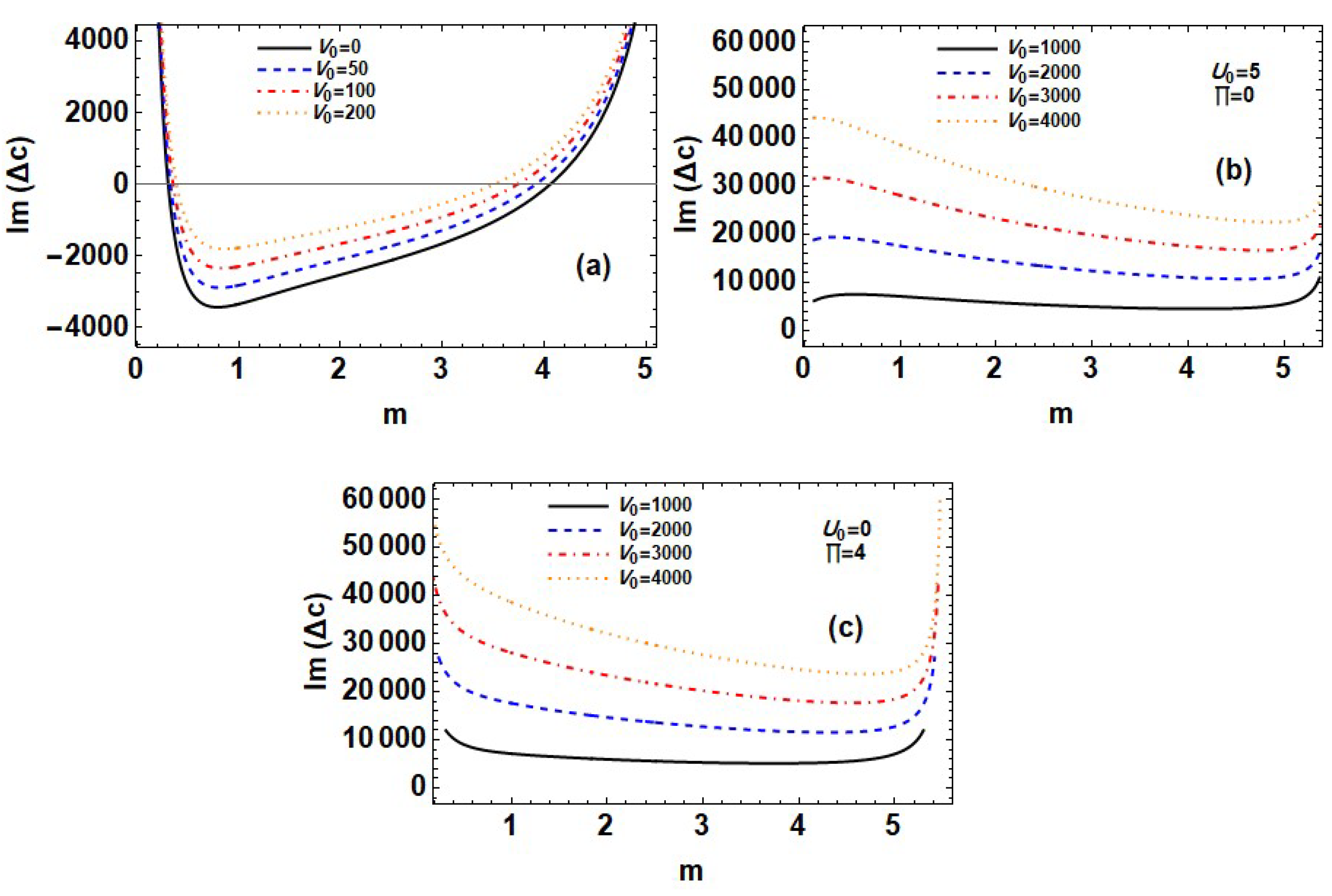
7.1. Effect of Velocity of Upper Rigid Boundary $U_0$

Figure 2 demonstrates the imaginary part of the complex wave speed $Im(\Delta c)$ against viscosity ratio m for various values of velocity of the upper rigid boundary $U_0$ and constant values of other physical quantities in the Poiseuille flow $U_0=0$ and Couette–Poiseuille flow $U_0>0$ cases. It is clear from the figure that when $U_0=0$, the system is unstable $[Im(\Delta c)>0]$ for values of $m\le 0.3$ and $m\ge 4.6$, while it is stable $[Im(\Delta c)<0]$ in the middle range of m. Increasing the velocity of upper rigid boundary $U_0$ leads to there being a critical value of the viscosity ratio $m=1$, before which $Im(\Delta c)$ values decrease, and after which $Im(\Delta c)$ values increase. Therefore, we draw the conclusion that the upper rigid boundary’s velocity plays a dual role in this system’s stability, stabilizing for $m<1$ and destabilizing for $m>1$ due to the decrease of the middle stability region.

7.2. Effect of Electric Potential Function $V_0$

Figure 3 illustrates the behavior of the imaginary part of the complex wave speed $Im(\Delta c)$ against viscosity ratio m for various values of electric potential function $V_0\ge 0$ and constant values of other physical quantities in (a) the general case of Couette–Poiseuille flow, (b) the Couette flow case, and (c) the Poiseuille flow case. It is clear from Figure 3a that in the absence of an electric field, the system is unstable $[Im(\Delta c)>0]$ for values of $m\le 0.3$ and $m\ge 4$, while it is stable $[Im(\Delta c)<0]$ in the middle range of m. Increasing the electric potential function $V_0$ leads to decreasing the middle range of m and keeping the behavior of the positive curves. Consequently, we draw the conclusion that the electric potential function destabilizes the system under consideration in the Couette–Poiseuille flow situation. It is clear also from Figure 3b for plane Couette flow and the absence of any pressure gradient, and also from Figure 3c for plane Poiseuille flow and presence of pressure gradient, respectively, that the system is always unstable, and consequently, the electric potential function has a destabilizing influence on the system, and the system in a plane Poiseuille flow with a pressure gradient is also more unstable than in a plane Couette flow with no pressure gradient. Finally, we draw the conclusion that the system without an electric field or a porous medium is more unstable than the system with them; see refs. [4,10].

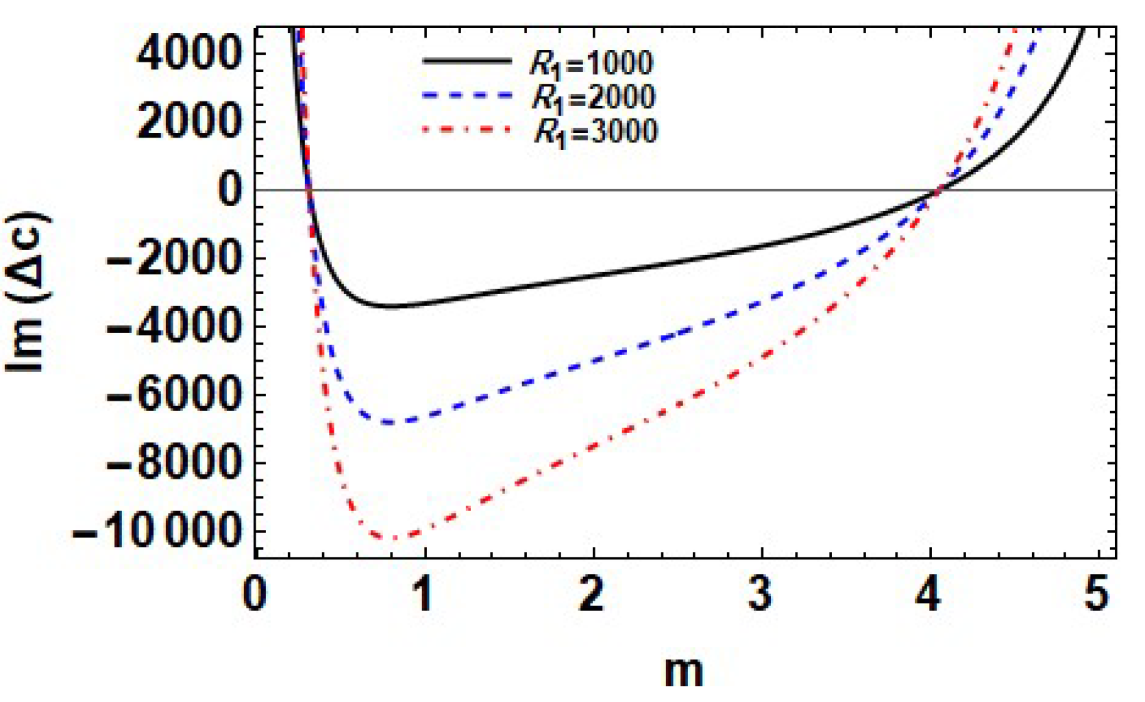
7.3. Effect of Reynolds Number $R_1$

Figure 4 gives the change of the imaginary part of the complex wave speed $Im(\Delta c)$ against viscosity ratio m for different values of Reynolds number $R_1$ and constant values of other physical parameters in the general case of Couette–Poiseuille flow. It is clear from the figure that for all values of Reynolds number, the system is neutrally stable $Im(\Delta c)=0$ at the viscosity ratios $m=0.3$ and $m=4$. By increasing the Reynolds number values, we observe that for the intervals $m<0.3$ and $m>4$, the system is slightly unstable and unstable, respectively, while in the middle region $0.3\le m\le 4$ values, we found that $Im(\Delta c)$ decreases at the same value of m. Due to the combination of viscosity, an electric field, and a porous material, we therefore draw the conclusion that the Reynolds number plays a dual role in the stability of the system under consideration.

7.4. Effect of Medium Permeability $K_1$

Figure 5 demonstrates the imaginary part of the complex wave speed $Im(\Delta c)$ against viscosity ratio m for various values of the medium permeability $K_1$ and constant values of other physical parameters. It is shown in the figure that the system is unstable $[Im(\Delta c)>0]$ for values of $m\le 0.1$ and $m\ge 5.7$, while it is stable $[Im(\Delta c)<0]$ in the middle range of m, and that the system is more stable when $m\approx 0.3$. Increasing the medium permeability of the porous media $K_1$ leads to decreasing the stability region in the middle range of viscosity ratio m. Hence, we declare that the medium permeability of porous medium $K_1$ has a destabilizing effect on the system for all values of m except in the range $0.6\le m\le 2.6$, where it has a stabilizing influence because in this range, $Im(\Delta c)$ decreases by increasing $K_1$ values.

7.5. Effect of Porosity of Porous Medium $\epsilon$

Figure 6 is drawn for the variation of the imaginary part of the complex wave speed $Im(\Delta c)$ versus viscosity ratio m for some values of porosity of the porous medium $\epsilon$ with constant values of the other parameters. It is clear from the figure that at a definite value of $\epsilon$, the generated curve behaves as if there are two branches above the horizontal axis where instability persists and one branch below the horizontal axis where stability conditions exist. It should be noted from the figure that in the first upper branch, the instability decreases with increasing $\epsilon$ values, and the second upper branch instability increases with increasing m values such that the stability range under the horizontal axis increases. Also take note of how nearly all of the curves have the same value. ($m\cong 1$), i.e., when the dynamic viscosities of the two fluids are equal. As a result, we draw the conclusion that the examined system is stabilized by the porosity of the porous medium $\epsilon$ because the stable range grows as the porosity does.

7.6. Effect of Dielectric Constant $ϵ$

Figure 7 illustrates the behavior of the imaginary part of the complex wave speed $Im(\Delta c)$ against viscosity ratio m for various values of the dielectric constant $ϵ\lessgtr 1$ and constant values of other physical quantities in the general case of Couette–Poiseuille flow through porous medium. It is clear from the figure that the system is unstable $[Im(\Delta c)>0]$ for values of $m\le 0.3$ and $m\ge 4$, while it is stable $[Im(\Delta c)<0]$ in the middle range of m. Increasing the dielectric constant $ϵ$ leads to slightly decreasing the middle range of m and keeping the behavior of the positive curves. Hence, we conclude that the dielectric constant $ϵ$ has a destabilizing influence of the considered, and that the system for values of $ϵ<1$ is more stable than for values of $ϵ\lessgtr 1$.

7.7. Effect of Upper to Lower Depth Ratio n

Figure 8 illustrates the behavior of the imaginary part of the complex wave speed $Im(\Delta c)$ against viscosity ratio m for various values of upper to lower depth ratio $n\lessgtr 1$, respectively, with constant values of other physical quantities in the general case of Couette–Poiseuille flow. It is clear from Figure 8a that for values where $n<1$, the system is unstable $[Im(\Delta c)>0]$ for values of $0.2<m\le 0.3$ and $m\ge 4$, while it is otherwise stable $[Im(\Delta c)<$0] for values of $m<0.2$ and also in the middle range of m. Increasing the upper to lower depth ratio $n<1$ leads to increasing the stable regions and also decreasing the unstable regions. Hence, we conclude that the upper to lower depth ratio $n<1$ has a dual role in the stability of the considered system, stabilizing as well as destabilizing depending on the viscosity ratio range. It is observed from Figure 8b that for small values of $n>1$, the system is unstable $[Im(\Delta c)>0]$ for values of upper to lower viscosity ratio $m\le 0.3$ and $m\ge 4$, while it is stable $[Im(\Delta c)<0]$ in the middle range of m. By increasing the values of upper to lower depth ratio n, the stability range increases and the imaginary part of the complex wave speed $Im(\Delta c)$ has more negative values, showing thereby that the middle stability region increases whatever the value of the upper to lower depth ratio is. Therefore, we conclude that the upper to lower depth ratio $n>1$ has a stabilizing influence on the system even in the presence of porous media in addition to the electric field.

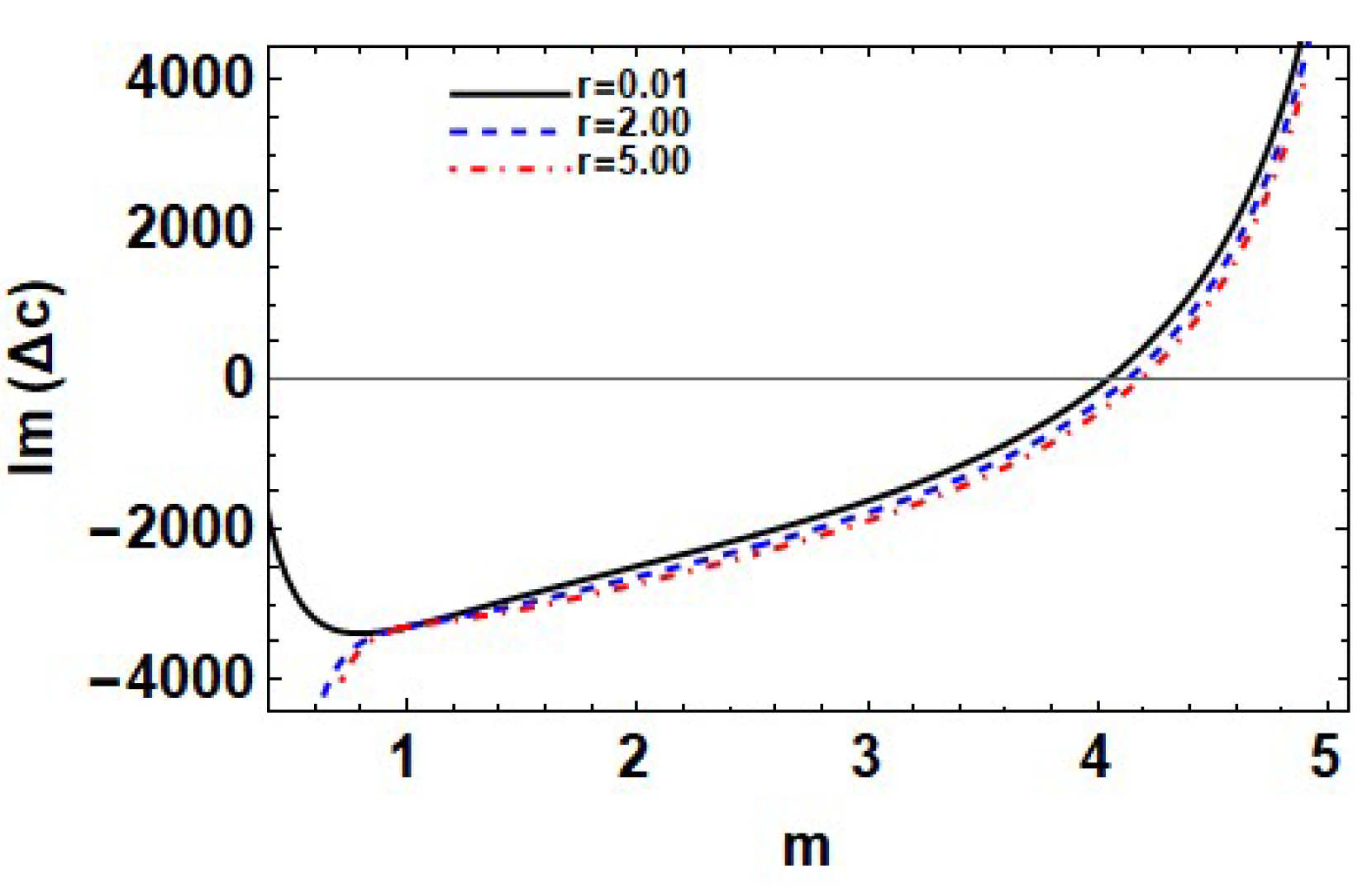
7.8. Effect of Upper to Lower Density Ratio r

Figure 9 depicts variations of the imaginary part of the complex wave speed $Im(\Delta c)$ against viscosity ratio m for various values of upper to lower density ratio $r\lessgtr 1$ with some values of the other parameters. It is clear from the figure that for small values of $0<r<1$, the system is stable $[Im(\Delta c)<0]$ in the viscosity ratio range $m<4$, and it is unstable $[Im(\Delta c)<0]$ afterwards. It is obvious also that for higher values of $r>1$, the corresponding imaginary part of the complex wave speed $Im(\Delta c)$ slightly decreases at any value of the viscosity ratio m. Hence, we conclude that for all values of $r\lessgtr 1$, the upper to lower density ratio has a stabilizing influence on this system.

7.9. Effect of Pressure Gradient $\Pi$

Figure 10 explores the variation of the imaginary part of the complex wave speed $Im(\Delta c)$ against viscosity ratio m for various values of pressure gradient $\Pi$ with some values of the other parameters. It is clear from the figure that at a definite value of $\Pi$, the generated curve behaves as if instability exists at two branches above the horizontal axis, and stability exists at one branch under the horizontal axis. It should be noted from the figure that in the first upper branch of instability, $Im(\Delta c)$ increases at the same value of m, and that the stability range under the horizontal axis decreases. Note also that all the curves coincide at $m\cong 1$, i.e., when the dynamic viscosities of the two fluids are equal. Therefore, we draw the conclusion that the pressure gradient destabilizes the system under study.

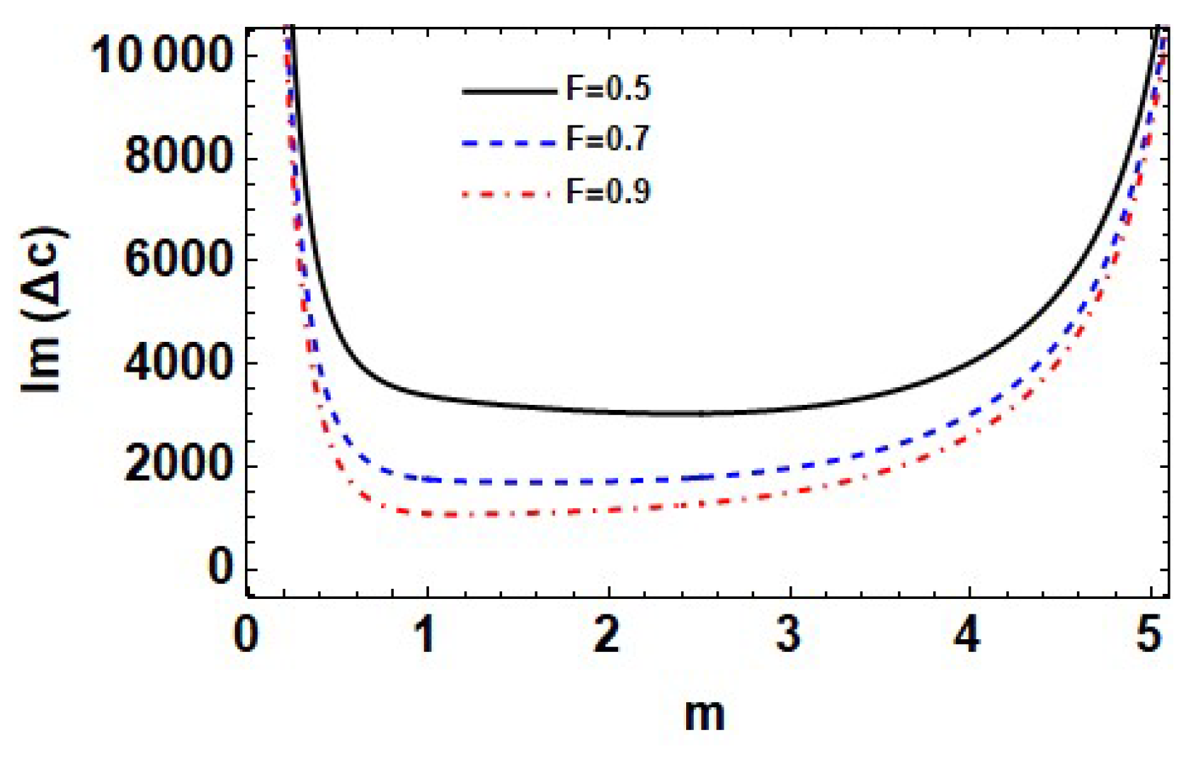
7.10. Effect of Froude Number F

Figure 11 shows the behavior of the imaginary part of the complex wave speed $Im(\Delta c)$ against viscosity ratio m for different values of Froude number F and constant values of other physical quantities in the general case of Couette–Poiseuille flow. It is clear from the figure that for small values of Froude number, the system is always unstable $Im(\Delta c)>0$ for all values of m, while by increasing Froude number F values, we found that $Im(\Delta c)$ decreases at the same value of m. Thus, we draw the conclusion that the Froude number stabilizes the Couette–Poiseuille flow system under consideration when a porous medium is present.

8. Concluding Remarks

In this paper, we investigated analytically the linear stability problem of the electrohydrodynamic plane Couette–Poiseuille flow of two superposed layers of fluids of different viscosities, densities and depths under the influences of electric field, porous medium and pressure gradient. The upper fluid is conducting while the lower one is dielectric, and the porous medium obeys the Brinkman model. We assumed that the amplitude of the perturbation was very small compared with the primary flow. With this supposition, the nonlinear Navier–Stokes equations are simplified to the linear Orr–Sommerfeld equation, which is solved in each fluid and coupled by the interface matching conditions. The approach of regular perturbations around the case of longer waves was utilized to solve the equations that resulted from this. The perturbation is determined to be neutrally stable in the first approximation where the linear inertial terms do not occur. The following conclusions can be obtained when the linear inertial factors are taken into account in the second approximation and unstable modes of the disturbance are discovered:

(1)

Critical values of the viscosity ratio distinguish the stabilizing and destabilizing effects of the velocity of the upper rigid boundary and Reynolds number on the stability of the system.

(2)

In the Couette–Poiseuille flow situation, the electric potential has a destabilizing effect on the system under consideration. As a result, the system is destabilizing in the presence of the electric field even if it is both stable and unstable when the electric field is absent. The electric potential has a destabilizing influence on the system for both the plane Couette flow and the plane Poiseuille flow cases, making the system for the plane Poiseuille flow case more unstable than in the plane Couette flow example.

(3)

The system is more unstable when a porous media and/or electric field are absent than when they are present.

(4)

For all values of the viscosity ratio m, the system is destabilized by the medium permeability of the porous medium except in the small range $0.6\le m\le 2.6$, where it has a stabilizing influence.

(5)

The examined system is stabilized by the porosity of the porous medium, and for various degrees of porosity, the related curves almost coincide at the same value of viscosity ratio $m\cong 1$.

(6)

The considered system is made unstable by the effects of the dielectric constant and pressure gradient, and the system for dielectric constant values $ϵ>1$ is more unstable than for dielectric constant values $ϵ<1$.

(7)

Depending on the range of viscosity ratios, the upper to lower depth ratio $n<1$ plays a dual role in the stability of the system under consideration, stabilizing as well as destabilizing, while it has a stabilizing influence on the system for $n>1$.

(8)

Since the stability ranges widen by raising their values, whatever they are, the upper to lower density ratio and Froude number have stabilizing effects on this system.

(9)

For each of the effects of velocity of the upper rigid boundary, porosity of porous medium, and upper to lower density ratio, the system with fluids of equal dynamic viscosities is found to be neutrally stable.

(10)

The viscosity stratification brings about a stabilizing as well as a destabilizing effect on the flow system.

Finally, using solutions of the eigenvalue problem for the long waves technique, and from the above findings and the corresponding figures, we have shown that our results recover previous studies in the absence of porous media [10], or the absence of electric field and porous media [4], and also for Couette or Poiseuille flow, alone. Similar Poiseuille flow instability problems in the absence of a pressure gradient have been studied using another technique (multiple-scales method) for dielectric/dielectric or conducting/dielectric fluids by El-Sayed ([53,54]) to investigate nonlinear analysis and solitary waves to obtain a nonlinear Schrodinger equation and their solitary wave solutions [53]. Also, we investigate the problem under the effect of a time-varying electric field to obtain a damped Mathieu equation with complex coefficients and to study both the resonance and non-resonance cases individually [54]. These studies show the importance of our model, which can be developed further for many other studies of physical and engineering interest.

At the end, we noticed that in many of the above-mentioned articles, which are limiting cases of our study [19,21,22,23,31,39] among others, the authors may solve the Orr–Sommerfeld equations using one of several numerical techniques described in the literature, e.g., Galerkin’s finite element method, the energy method, the Chebyshev spectral collection method along with the QZ algorithm, … etc. But in our study, to solve the obtained Orr–Sommerfeld equations, an asymptotic analysis is conducted for wave numbers in the long wavelength limit, and we obtained excellent results for the stability of the considered system; to the best of our knowledge, no attempts have been made in a similar way. This asymptotic method is very effective and it was used more recently by some authors; see refs. [49,50,55]. From the results, it is clear that by adjusting the many factors affecting the flow designs, one can exert more control over the system under consideration. By boosting or suppressing instability where it is desired or unwanted, this trait can be efficiently used in the right applications.

References

1. Joseph, D.D.; Renardy, Y.Y. Fundamentals of Two-Fluid Dynamics; Part I: Mathematical Theory and Applications; Springer: New York, NY, USA, 1993. [Google Scholar]
2. Yih, C.-S. Instability of liquid flow down an inclined plane. Phys. Fluids 1963, 6, 321–334. [Google Scholar] [CrossRef] [Green Version]
3. Smith, M.K. The long-wave interfacial instability of two liquid layers stratified by thermal conductivity in an inclined channel. Phys. Fluids 1995, 7, 3000–3012. [Google Scholar] [CrossRef]
4. Yih, C.-C. Instability due to viscosity stratification. J. Fluid Mech. 1967, 27, 337–352. [Google Scholar] [CrossRef]
5. Shlang, T.; Sivashinsky, G.I.; Bahchin, A.J.; Frenkel, A.I. Irregular wavy flow due to viscosity stratification. J. Phys. 1985, 46, 863–866. [Google Scholar] [CrossRef]
6. Hooper, A.P. Long-wave instability at the interface between two viscous fluids: Thin layer effect. Phys. Fluids 1985, 28, 1613–1618. [Google Scholar] [CrossRef]
7. Charru, F.; Fabre, J. Long waves at the interface between two viscous fluids. Phys. Fluids 1994, 6, 1223–1235. [Google Scholar] [CrossRef]
8. Tilley, B.S.; Davies, S.H.; Bankoff, S.G. Linear stability theory of two-layer fluid flow in an inclined channel. Phys. Fluids 1994, 6, 3906–3922. [Google Scholar] [CrossRef]
9. Merkt, D.; Pototsky, A.; Bestehon, M.; Thiele, U. Long-wave theory of bounded two-layer films with a free liquid-liquid interface: Short- and long-time evolution. Phys. Fluids 2005, 17, 064104. [Google Scholar] [CrossRef] [Green Version]
10. Mohamed, A.A.; Elshehawey, E.F.; El-Sayed, M.F. Electrohydrodynamic stability of two superposed viscous fluids. J. Colloid Interface Sci. 1995, 109, 65–78. [Google Scholar] [CrossRef]
11. El-Sayed, M.F.; Moatimid, G.M.; Metwaly, T.M.N. Nonlinear electrohydrodynamic stability of two superposed streaming finite dielectric fluids in porous medium with interfacial surface charges. Transp. Porous Med. 2011, 86, 559–578. [Google Scholar] [CrossRef]
12. El-Sayed, M.F.; Moussa, M.H.M.; Hassan, A.A.A.; Hafez, N.M. Electrohydrodynamic instability of plane Couette-Poiseuille flow of three superposed viscous stratified dielectric fluid layers. Int. J. Appl. Math. Mech. 2013, 9, 13–50. [Google Scholar]
13. Kao, T.W.; Park, C. Experimental investigations of stability of the channel flows. Part 2. Two layered Co-current flow in a rectangular channel. J. Fluid Mech. 1972, 52, 401–423. [Google Scholar] [CrossRef]
14. Yiantsios, S.G.; Higgins, B.G. Linear stability of plane Poiseuille flow of two superposed fluids. Phys. Fluids 1988, 31, 3225–3238, Erratum in Phys. Fluids A 1989, 1, 897. [Google Scholar] [CrossRef]
15. Sadoghi, V.M.; Higgins, B.G. Stability of sliding Couette-Poiseuille flow in an annulus subject to axisymmetric and asymmetric disturbances. Phys. Fluids A 1991, 3, 2092–2104. [Google Scholar] [CrossRef]
16. Hooper, A.P. The stability of two superposed viscous fluids in a channel. Phys. Fluids A 1989, 1, 1133–1142. [Google Scholar] [CrossRef]
17. South, M.J.; Hooper, A.P. Linear growth in two-fluid plane Poiseuille flow. J. Fluid Mech. 1999, 381, 121–139. [Google Scholar] [CrossRef]
18. You, X.Y.; Zhang, X.; Chen, X. On linear stability of plane Poiseuille flow of two viscosity-stratified liquids. J. Taiwan Univ. 2005, 38, 1017–1020. [Google Scholar]
19. Chokshi, P.; Gupta, S.; Yadav, S.; Agrawal, A. Interfacial instability in two-layer Couette-Poiseuille flow of viscoelastic fluids. J. Non-Newton. Fluid Mech. 2015, 224, 17–29. [Google Scholar] [CrossRef]
20. Chattopadhyay, G.; Usha, R. On the Yih-Marangoni instability of two-phase Poiseuille flow in a hydrophobic channel. Chem. Eng. Sci. 2016, 145, 214–232. [Google Scholar] [CrossRef]
21. Ghosh, S.; Behera, H. Instability mechanism for miscible two-fluid channel flow with wall slip. Z. Angew. Math. Mech. 2018, 98, 1947–1958. [Google Scholar] [CrossRef]
22. Chattopadhyay, G.; Ranganathan, U.; Millet, S. Instability in viscosity-stratified two-fluid channel flow over an anisotropic-inhomogeneous porous bottom. Phys. Fluids 2019, 31, 012103. [Google Scholar] [CrossRef]
23. Govindarajan, R.; Sahu, K.C. Instabilities in viscosity-stratifed fow. Annu. Rev. Fluid. Mech. 2014, 46, 331–353. [Google Scholar] [CrossRef]
24. Melcher, J.R.; Taylor, G.I. Electrohydrodynamics: A review of the role of the interfacial shear stresses. Annu. Rev. Fluid Mech. 1969, 1, 111–146. [Google Scholar] [CrossRef]
25. Thaokar, R.M.; Kumaran, V. Electrohydrodynamic instability of the interface between two fluids confined in a channel. Phys. Fluids 2005, 17, 084104. [Google Scholar] [CrossRef]
26. Ozen, O.; Aubry, N.; Papageorgiou, D.T.; Petropoulos, P.G. Electrohydrodynamic linear stability of two immiscible fluids in channel flow. Electrochim. Acta 2006, 51, 5316–5323. [Google Scholar] [CrossRef]
27. Zahn, J.D.; Reddy, V. Two phase micromixing and analysis using electrohydrodynamic instabilities. Microfluid. Nanofluid. 2006, 2, 399–415. [Google Scholar] [CrossRef]
28. Melcher, J.R. Continuum Electromechanics; MIT Press: Cambridge, MA, USA, 1981. [Google Scholar]
29. Li, F.; Ozen, O.; Aubry, A.; Papageorgiou, D.T.; Petropoulos, P.G. Linear stability of a two-fluid interface for electrohydrodynamic mixing in a channel. J. Fluid Mech. 2007, 583, 347–377. [Google Scholar] [CrossRef]
30. Ersoy, G.; Uguz, A.K. Electro-hydrodynamic instability in a microchannel between a Newtonian and non-Newtonian liquid. Fluid Dyn. Res. 2012, 44, 031406. [Google Scholar] [CrossRef]
31. Ozan, S.C.; Uguz, A.K. Nonlinear evolution of the interface between immiscible fluids in a micro channel subjected to an electric field. Eur. Phys. J. Spec. Top. 2017, 226, 1207–1218. [Google Scholar] [CrossRef]
32. Kaykanat, S.I.; Uguz, A.K. The linear stability between a Newtonian and a power-law fluid under a normal electric field. J. Non-Newton. Fluid Mech. 2020, 277, 104220. [Google Scholar] [CrossRef]
33. Zhang, J.; Zahn, J.D.; Lin, H. A general analysis for the electrohydrodynamic instability of stratified immiscible fluids. J. Fluid Mech. 2011, 681, 293–310. [Google Scholar] [CrossRef]
34. Altundemir, S.; Eribol, P.; Uguz, A. Droplet formation and its mechanism in a microchannel in the presence of an electric field. Fluid Dyn. Res. 2018, 50, 051404. [Google Scholar] [CrossRef]
35. Papageorgiou, D.T.; Petropoulos, P.G. Generation of interfacial instabilities in charged electrified viscous liquid films. J. Eng. Math. 2004, 50, 223–240. [Google Scholar] [CrossRef]
36. Eribol, P.; Uguz, A.K. Experimental investigation of electrohydrodynamic instabilities in micro channels. Eur. Phys. J. Spec. Top. 2015, 224, 425–434. [Google Scholar] [CrossRef]
37. Li, H.; Wong, T.N.; Nguyen, N.T. Electrohydrodynamic and shear-stress interfacial instability of two streaming viscous liquid inside a microchannel for tangential electric fields. Micro Nanosyst. 2012, 4, 14–24. [Google Scholar]
38. Li, H.; Wong, T.N.; Nguyen, N.T. Instability of pressure driven viscous fluid streams in a microchannel under a normal electric field. Int. J. Heat Mass Transf. 2012, 55, 6994–7004. [Google Scholar] [CrossRef] [Green Version]
39. Eribol, P.; Kaykanat, S.I.; Ozan, S.C.; Uguz, A.K. Electrohydrodynamic instability between three immiscible fluids in a microchannel: Lubrication analysis. Micrdfluid. Nanofluid. 2022, 26, 16. [Google Scholar] [CrossRef]
40. Bejan, A. Porous and Complex Flow Structure in Modern Technology; Springer: Berlin/Heidelberg, Germany, 2004. [Google Scholar]
41. Straughan, B. Stability and Wave Motion in Porous Media; Applied Mathematical Sciences; Springer: New York, NY, USA, 2008. [Google Scholar]
42. Nield, D.A.; Bejan, A. Convection in Porous Medium, 4th ed.; Springer: New York, NY, USA, 2013. [Google Scholar]
43. Allen, M.B., III; Behie, G.A.; Trangenstein, J.A. Multiphase Flow in Porous Media: Mechanics, Mathematics, and Numerics; Springer: New York, NY, USA, 2013. [Google Scholar]
44. Del Rio, J.A.; Whitaker, S. Electrohydrodynamics in Porous Media. Tranp. Porous Med. 2001, 44, 385–405. [Google Scholar] [CrossRef]
45. Liu, R.; Liu, Q.S.; Zhao, S.C. Instability of plane Poiseuille flow in a fluid-porous system. Phys. Fluids 2008, 20, 104105. [Google Scholar] [CrossRef] [Green Version]
46. El-Sayed, M.F. Electrohydrodynamic instability of two superposed viscous streaming fluids through porous media. Can. J. Phys. 1997, 75, 499–508. [Google Scholar] [CrossRef]
47. Eldabe, N.T. Electrohydrodynamic stability of two stratified power law liquids in couette fow. Nuovo C. B 1988, 101, 221–235. [Google Scholar] [CrossRef]
48. Goyal, H.; Kumar, A.A.P.; Bandyopadhay, D.; Usha, R.; Banerjee, T. Instability of confined two-layer flow on a porous medium: An Orr-Sommerfeld analysis. Chem. Eng. Sci. 2013, 97, 109–125. [Google Scholar] [CrossRef]
49. Chimetta, B.R.; Franklin, E.M. Asymptotic and numerical solutions of the Orr-Sommerfeld equation for a thin liquid film on an inclined plane. In Proceedings of the IV Journeys in Multiphase Flows (JEM2017), Sao Paulo, Brazil, 27–31 March 2017. [Google Scholar]
50. Ramakrishnan, V.; Mushthaq, R.; Roy, A.; Vengadesan, S. Stability of two-layer flows past slippery surfaces. I. Horizontal channels. Phys. Fluids 2021, 33, 084112. [Google Scholar] [CrossRef]
51. Zakhvataef, V.E. Longwave instability of two-layer dielectric fluid flows in a transverse electrostatic field. Fluid Dyn. 2000, 35, 191–199. [Google Scholar] [CrossRef]
52. Zakaria, K.; Alkharashi, S.A. Modeling and analysis of two electrified films flow traveling down between inclined permeable parallel substrates. Acta Mech. 2017, 228, 2555–2581. [Google Scholar] [CrossRef]
53. El-Sayed, M.F. Nonlinear analysis and solitary waves for two superposed streaming electrified fluids of uniform depths with rigid boundaries. Arch. Appl. Mech. 2008, 78, 663–685. [Google Scholar] [CrossRef]
54. El-Sayed, M.F. Instability of two streaming conducting and dielectric bounded fluids in porous medium under time-varying electric field. Arch. Appl. Mech. 2009, 79, 19–39. [Google Scholar] [CrossRef]
55. Hussain, Z.; Khan, N.; Gul, T.; Ali, M.; Shahzad, M.; Sultan, F. Instability of magnetohydrodynamic Couette flow for electrically conducting fluid through porous media. Appl. Nanosci. 2020, 10, 5125–5134. [Google Scholar] [CrossRef]
Figure 1. Definition sketch of the problem.
Mathematics 11 03281 g001
Figure 2. Variation of the imaginary part of the complex wave speed Im ( Δ c ) against viscosity ratio m for various values of velocity of the upper rigid boundary U 0 and constant values of other physical quantities.
Mathematics 11 03281 g002
Figure 3. Variation of the imaginary part of the complex wave speed Im ( Δ c ) against viscosity ratio m for various values of electric potential function V 0 and constant values of other physical quantities.
Mathematics 11 03281 g003
Figure 4. Variation of the imaginary part of the complex wave speed Im ( Δ c ) against viscosity ratio m for various values of Reynolds number R 1 and constant values of other physical parameters.
Mathematics 11 03281 g004
Figure 5. Variation of the imaginary part of the complex wave speed Im ( Δ c ) against viscosity ratio m for some values of medium permeability K 1 and constant values of other physical parameters.
Mathematics 11 03281 g005
Figure 6. Variation of the imaginary part of the complex wave speed Im ( Δ c ) against viscosity ratio m for some values of porosity of the porous medium ε with constant values of the other parameters.
Mathematics 11 03281 g006
Figure 7. Variation of the imaginary part of the complex wave speed Im ( Δ c ) against viscosity ratio m for various values of the dielectric constant ϵ and constant values of other physical quantities.
Mathematics 11 03281 g007
Figure 8. Variation of the imaginary part of the complex wave speed Im ( Δ c ) against viscosity ratio m for various values of upper to lower depth ratio n and constant values of other physical quantities.
Mathematics 11 03281 g008
Figure 9. Variation of the imaginary part of the complex wave speed Im ( Δ c ) against viscosity ratio m for various values of velocity of upper to lower density ratio r with some values of the other parameters.
Mathematics 11 03281 g009
Figure 10. Variation of the imaginary part of the complex wave speed Im ( Δ c ) against viscosity ratio m for various values of velocity of pressure gradient Π with some values of the other parameters.
Mathematics 11 03281 g010
Figure 11. Variation of the imaginary part of the complex wave speed Im ( Δ c ) against viscosity ratio m for various values of Froude number F and constant values of other physical quantities.
Mathematics 11 03281 g011
Disclaimer/Publisher’s Note: The statements, opinions and data contained in all publications are solely those of the individual author(s) and contributor(s) and not of MDPI and/or the editor(s). MDPI and/or the editor(s) disclaim responsibility for any injury to people or property resulting from any ideas, methods, instructions or products referred to in the content.