Article

Design of a Fixed-Time Stabilizer for Uncertain Chaotic Systems Subject to External Disturbances

1
Department of Mathematics, Faculty of Sciences, University of Zanjan, Zanjan 45371-38791, Iran
2
Department of Electrical Engineering, Faculty of Engineering, University of Zanjan, Zanjan 45371-38791, Iran
3
Graduate School of Intelligent Data Science, National Yunlin University of Science and Technology, Douliou 64002, Yunlin, Taiwan
4
Department of Electrical and Computer Engineering, University of Louisiana at Lafayette, Lafayette, LA 70504, USA
5
Department of Cyber-Physical Systems, St. Petersburg State Marine Technical University, 190121 Saint-Petersburg, Russia
*
Author to whom correspondence should be addressed.
Mathematics 2023, 11(15), 3273; https://doi.org/10.3390/math11153273
Submission received: 3 July 2023 / Revised: 21 July 2023 / Accepted: 24 July 2023 / Published: 25 July 2023

Abstract

:
This paper addresses the fixed-time stability problem of chaotic systems with internal uncertainties and external disturbances. To this end, new sliding-mode surfaces are introduced to design fixed-time controllers for the stabilization of perturbed chaotic systems. First, the required conditions for deriving fixed-time stability are determined. Then, using the obtained stability theorems and sliding mode techniques, the controllers are synthesized. The proposed controller enables the convergence of the trajectories of the chaotic system to the origin in finite time, independently of the initial conditions. The performance of the proposed approach is assessed using a simulation study of a PMSM system and the Matouk system. Among the advantages of the proposed controller are its robustness to external disturbances and the boundedness of the settling time to a constant value for any initial condition.
MSC:
37D45; 39A33; 34H10; 93Dxx; 93D09; 93D40; 93C10

1. Introduction

Chaotic dynamics are encountered in many engineering applications, such as network systems, digital communications, mechanical systems, organic phenomena for example biological populations, and so on [1,2,3,4]. These dynamical systems have several unique characteristics, such as randomness, non-periodicity, and high sensitivity to the initial values. For instance, reference [5] demonstrates that the simple-model regulation of plant and animal populations is inherently nonlinear and subject to uncertain chaotic dynamics. In 1990, a discrete control algorithm, dubbed the OGY method [6], was established to control the chaos. The same year, the work [7] put out a principle to synchronize chaotic systems by connecting them with standard signals. It considered the signs of Lyapunov exponents and applied them to synchronize chaotic systems. In 2000, reference [8] proposed a power integrator to address the problem of robust stabilization for a class of uncertain nonlinear systems. In the same year, for the equilibrium of a continuous dynamical system, the finite-time stability for a system was defined in [9]. Since then, several research initiatives have been made to examine chaotic synchronization, and they have produced remarkable results. A technique for the finite-time synchronization of two different chaotic systems with unknown parameters was first presented in 2011 [10]. In 2012, the research [11] proposed two different nonlinear control strategies for uncertain linear dynamics. The objective was to provide global finite-time stability regardless of the initial conditions. To ensure finite-time and fixed-time stability for nonlinear systems, reference [12] developed a number of theorems based on Implicit Lyapunov Functions in 2015. A method for regulating dynamical systems with internal uncertainties, external disturbances, and chaotic behavior was put out by [13] in 2016. In order to synchronize the modified Chua’s chaotic system, the approach was then generalized for the control of chaotic systems. In 2017, the work [14] highlighted the importance of chaotic dynamics in network systems and proposed some novel methods for controlling the uncertain chaotic behavior in network systems. The same year, [15] proposed a technique to synchronize and stabilize a certain class of chaotic systems that are subject to both internal uncertainties and external disturbances. In addition, [16] created an adaptive dynamic surface in 2017 to control a type of strict-feedback nonlinear system with complete state restrictions and unmodeled dynamics. This study [17] in 2018 proposed a novel, robust tracking control system for robot manipulators with dynamic uncertainties and unknown disturbances. The technique is carried out by developing two adaptive interval type-2 fuzzy logic systems to better approximate the parametric uncertainties of the nominal system. Following that, a novel control algorithm based on a newly synthesized fuzzy sliding mode control law was proposed. Ref. [18] presented a unique hyperchaotic system consisting of four-dimensional dynamical systems with continuous-time ordinary differential equations and three quadratic nonlinearities for the first time in 2019. They also proposed a method to suppress the chaotic behavior in this system based on the Lyapunov stability approach. Additionally, [19] proposes a technique based on backstepping and Lyapunov predictive control to synchronize nonlinear systems in order to guarantee the boundedness of the solution for the perturbed system. In the same year, [20] introduced an adaptive sliding mode disturbance observer-based finite time control approach for uncertain nonlinear systems. In addition, [21] established various criteria for the resilient management and synchronization of a class of 3D fractional-order chaotic systems with external disturbances in 2019. A class of ambiguous single-input, single-output nonlinear systems with unclear control direction and disturbances was taken into consideration in [22]. It designed new controllers and adaptive laws and demonstrated that all the variables in the closed-loop system are constrained, and the tracking error converges to the origin. In that year, [23] introduced various approaches based on continuous strategies for solving the problem of finite time and fixed time synchronization of complicated networks. In 2020, for the first time, [24] presented a novel control approach to suppress the chaotic phenomenon in a PI control system. In [25], the issue of finite-time synchronization of a type of chaotic master and slave system with unknown parameters, uncertainties, and disturbances was examined. In addition, numerous effective control strategies have been suggested to synchronize the chaotic dynamics. For example, in 2020, [26] derived a new fixed-time stability theorem for the synchronization of chaotic dynamics. Moreover, [27] used sliding mode control and Lyapunov stability to offer several sufficient conditions to stabilize a globally nonlinear system. Ref. [28] considered the fixed-time control problem of perturbed chaotic systems. Ref. [29] developed a novel analytical technique to synchronize nonlinear systems with stochastic perturbations. However, the setting time was not only dependent on the gains and initial conditions but also on the controlled and uncontrolled widths. Simultaneously, [30] proposed a new hybrid-driven sampling control strategy for the finite-time synchronization of complex networks with stochastic cyber-attacks. In recent papers, authors have profoundly researched the finite-time synchronization of complex network systems. They used Lyapunov functions and the inequality technique. Based on the above-mentioned studies, it is evident that the systems’ initial conditions have fundamental importance in the determination of fixed-time stability. The settling time will be considerable if the initial values are large enough, a situation that is not suitable for engineering applications. To alleviate this problem, [31] proposed a different analysis method for the finite-time synchronization of the drive-response inactive neural networks with mixed time-varying delays. A new inequality method was proposed to yield better response dynamics while achieving fixed-time stability. In 2021, [32] presented some sufficient conditions to guarantee the finite-time stability of time-varying systems. Ref. [33] proposed a method for the fast finite-time stability of a class of stochastic nonlinear systems. Based on the Lyapunov theorem and some inequality techniques, sliding mode surfaces were proposed to establish controllers that guarantee fixed-time stability independently of the system’s initial conditions. In 2022, [34] proposed a criterion that determines a boundary for the fixed-time stability of chaotic dynamics with internal uncertainties and external disturbances. In that year, the article [35] addressed the topic of employing a dynamic sliding mode controller to stabilize interval type-2 fuzzy systems with uncertainties, time delays, and external disturbances. When designing controls, the sliding surface function is employed. The reachability of the surface of the addressed sliding mode is first shown. Second, the necessary requirements for the stability of the system and the suggested control scheme are derived. Ref. [36] derived the criterion for finite-time stability of stochastic systems represented by fractional-order delay differential equations. Ref. [37] used a type of inequality to guarantee the finite-time stability of state-dependent delayed systems. Ref. [38] developed some sufficient criteria for the finite-time stability of linear systems in the fractional domain with time-varying delays. Ref. [39] considered some inequalities and the Lyapunov-Krasovskii functional method to investigate the finite-time stability of singular systems with time delays. Ref. [40] developed and presented a vital theory for the finite-time stability of a class of stochastic nonlinear systems. Ref. [41] suggested sufficient conditions for the finite-time and fixed-time stability of non-autonomous ODE systems. In most of the papers mentioned above, the main problem is the control of a chaotic system with uncertainty and disturbances. The methods used in these articles are often based on the boundary assumption of uncertainty and disturbances under certain initial conditions. These articles frequently take into account the common sliding surface, and by using matrix inequalities, methods for adaptive and optimal control, fuzzy control, and other techniques, under the assumption that the boundary of disturbances and particular initial conditions have been known, an appropriate solution to the problem has been identified. Although these approaches are theoretically efficient, the primary difficulty with them is that the boundary assumption of disturbances and certain initial conditions cannot be neglected. As these methods reveal, the problem becomes more difficult if we consider fixed-time stability. The difficulty, in our opinion, stems from the fact that the appropriate sliding surface is not addressed in the controller design. In this research, we suggested a sliding surface and constructed controllers based on it to deal with the problem of unbounded perturbations as well as arbitrary initial conditions. These controllers are constructed in a way that removes the impacts of uncertainty and disturbances, whether they are bounded or unbounded.
This paper addresses the fixed-time stability problem of chaotic systems with internal uncertainties and external disturbances. Its main contributions are as follows:
  • It designs a fixed-time controller for the stabilization of perturbed chaotic systems based on a new sliding mode surface.
  • It suggests a method to determine a boundary for the fixed-time stability of uncertain chaotic systems with external disturbances that is independent of the initial conditions.
  • It derives the required conditions to achieve the fixed-time stability.
The remainder of the paper is organized as follows. Some preliminaries are given in Section 2. The controller design is detailed in Section 3. Numerical simulations illustrating the performance of the proposed approach are given in Section 5. Finally, some conclusions are drawn in Section 5.

2. Preliminaries and System Description

Consider the following dynamical system:
x ˙ 1 = f 1 x + f 1 x + δ 1 ( x ) x ˙ 2 = f 2 x + f 2 x + δ 2 ( x ) x ˙ n = f n x + f n x + δ n ( x )
where i 1,2 , . , n , x i is the state vector, δ i x denotes the external disturbances, f i ( x ) refers to the internal uncertainties, and f i ( x ) is a continuous function. It is essential to first present some lemmas and definitions for system (1).
Definition 1 [27]: 
An autonomous differential equation:
f : R n R n ,     x ˙ t = f x t   ,     x 0 = x 0
is said to be fixed-time stable if
  t       t > t   ; x t = 0         lim t t x t = 0
t  is independent of the initial value of the autonomous differential equation.
Lemma 1: 
Suppose that  K > 0 and  x : R R  is a continuous differentiable function that satisfies the following conditions:
x ˙ = K   s i g n x x + 1 x + 1 2 1         ,         x 0 = x 0
Then, origin of system (4) is fixed-time stable and setting time is t π K .
Proof: 
It follows from the (4) that:
d x d t = K   s i g n x x + 1 x + 1 2 1
Thus
d x   s i g n x x + 1 x + 1 2 1 = K   d t
So
x ( 0 ) x ( t ) d x   s i g n x x + 1 x + 1 2 1 = K 0 t d τ
After evaluating the integrals, the following result is obtained:
2 t a n 1 s i g n ( x ) x + 2 x .   s i g n ( x ) + x 2 s i g n ( x ) x ( 0 ) x ( t ) = K t
But, for any θ , we know that 2 t a n 1 ( θ )   π ; thus t π K , there exists a fixed time t such that lim t t x t = 0 . The convergence time t is given by t π K . Therefore, Equation (4) is fixed-time stable. □
Remark 1: 
In article [34], the setting time is defined by five parameters with limitations, while in this article, the setting time is set by only one parameter. Therefore, in terms of applicability, Lemma 1 has some advantages over Theorem 1 presented in paper [34].
For example, if K = 2 and x ˙ = K   s i g n x x + 1 x + 1 2 1 ,   x 0 = 7 . Figure 1 shows that the graph of x ( t ) is a continuous differentiable function, and the setting time is t π 2 .
Also, if placed K = 1 2 and x 0 = 3 , similar results are obtained. Figure 2 shows that the setting time is less than t 2 π .

3. Sliding Surface and Controller Design

This section focuses on designing a controller for the dynamical system defined by (9):
x ˙ 1 = f 1 x + f 1 x + δ 1 x + u 1 ( t ) x ˙ 2 = f 2 x + f 2 x + δ 2 ( x ) + u 2 ( t ) x ˙ n = f n x + f n x + δ n ( x ) + u n ( t )
where i 1,2 , . , n , x i is the state vector, δ i x denotes the external disturbances, f i ( x ) shows the internal uncertainties, and f i ( x ) is a continuous function, u i ( t ) denotes the controller. We want to design u i ( t ) , such that (9) is fixed-time stable.
Remark 2: 
In article [34], it is assumed that the external disturbances  f i ( x ) and the internal uncertainties  δ i x  are bounded, while this article does not use such an assumption.
In this section, a new sliding mode controller is planned to realize the fixed-time stable control of nonlinear system. There are two principal steps in the design technique of the suggested fixed-time controller:
  • constructing a suitable nonsingular terminal sliding surface.
  • building a robust fixed-time control law to guarantee the existence of the sliding motion in a given setting time.
To realize the control of the system (9), the nonlinear sliding mode is constructed as:
s i = x i + 0 t K   s i g n x i x i + 1 x i + 1 2 1
If the states arrive at the sliding surface, then s i = 0 , s ˙ i = 0 .
Theorem 1: 
Consider the sliding mode dynamics (10). This system is fixed-time stable and its trajectories converge to the equilibrium  x t = 0 in a setting time  T 1  which is determined by T 1 π K .
Proof: 
Define the following Lyapunov function:
V t = 1 2 i = 1 n x i 2
Calculation of derivative of V t with respect to t yields:
V ˙ = i = 1 n x i x ˙ i         = i = 1 n x i K   s i g n x i x i + 1 x i + 1 2 1         = K i = 1 n x i   s i g n x i x i + 1 x i + 1 2 1
But x i s i g n x i x i + 1 x i + 1 2 1 0 , thus V ˙ 0 .
According to Lyapunov theorem x i 0 . However,
x ˙ i = K   s i g n x i x i + 1 x i + 1 2 1 , thus, by means of Lemma 1, it is clear that setting time is T 1 π K , and (10) is fixed-time stable. □
If s i 0 , it means the states of system (9) is outside of the sliding mode surface. We should then design an appropriate controller to put the states into the sliding surface and make it remain there constantly. For this aim, the following theorem is provided.
Theorem 2: 
Assume that
u i = ξ i K   s i g n x i x i + 1 x i + 1 2 1 f i x f i ( x ) δ i x    
With
ξ i = K   s i g n s i s i + 1 s i + 1 2 1
is a controller, then (9) is fixed-time stable. The convergence time  t  is:
T 2 2 π K
where the parameter satisfies  K > 0 .
Proof: 
In the same way, we choose the Lyapunov function as:
V t = 1 2 i = 1 n s i 2
calculating the derivative of both sides of V , one has:
V ˙ = i = 1 n s i s ˙ i         = i = 1 n s i x ˙ i + K   s i g n x i x i + 1 x i + 1 2 1         = i = 1 n s i K   s i g n x i x i + 1 x i + 1 2 1 + i = 1 n s i f i x + f i x + δ i ( x ) + u i ( t )
Substituting the controller in the above equation yields:
V ˙ = i = 1 n s i K   s i g n x i x i + 1 x i + 1 2 1       i = 1 n s i K   s i g n x i x i + 1 x i + 1 2 1       i = 1 n s i K   s i g n s i s i + 1 s i + 1 2 1      
Simplifying the above equation yields:
V ˙ = K i = 1 n s i   s i g n s i s i + 1 s i + 1 2 1
But s i s i g n s i s i + 1 s i + 1 2 1 0 , thus V ˙ 0 .
According to Lyapunov’s theorem s i 0 . However, s ˙ i = s i   s i g n s i s i + 1 s i + 1 2 1 , thus, by means of Lemma 1, it is clear that setting time is T 1 π K . It follows from the Theorem 1 that when the trajectories are placed on the sliding surface s i = 0 , it takes a maximum of π K seconds to reach the origin; therefore, the system is fixed-time stable, and setting time T 2 is determined by T 2 2 π K . □
Remark 3: 
The basis of finding a fixed time is related to finding a differential equation  x ˙ = F ( x ) , such that it satisfies the expectations of Lemma 1. Also, the control structure in this paper is not only unrelated to the system parameters but also independent of the initial values. The method described here can be suitable for more general chaotic dynamics.

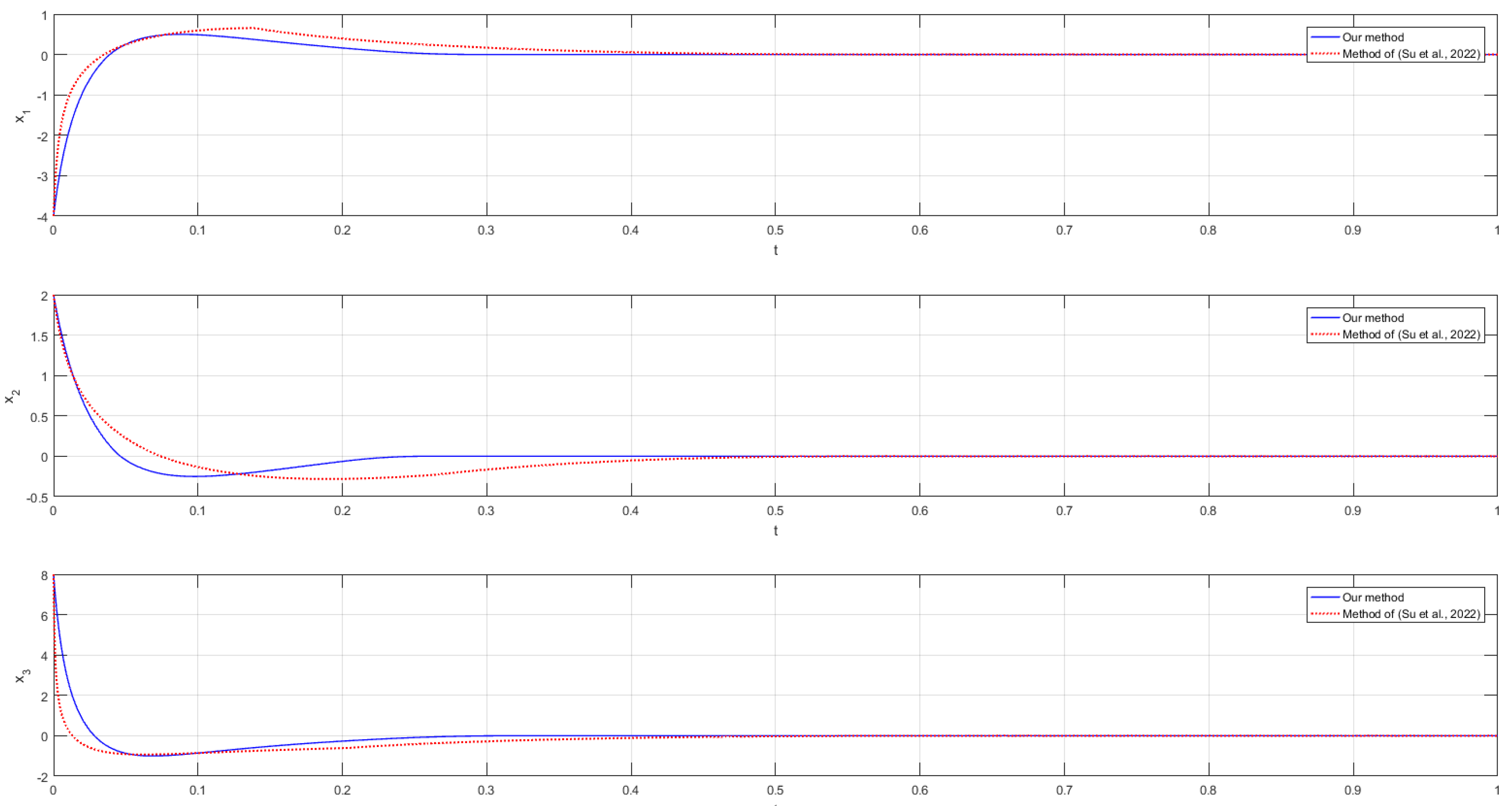
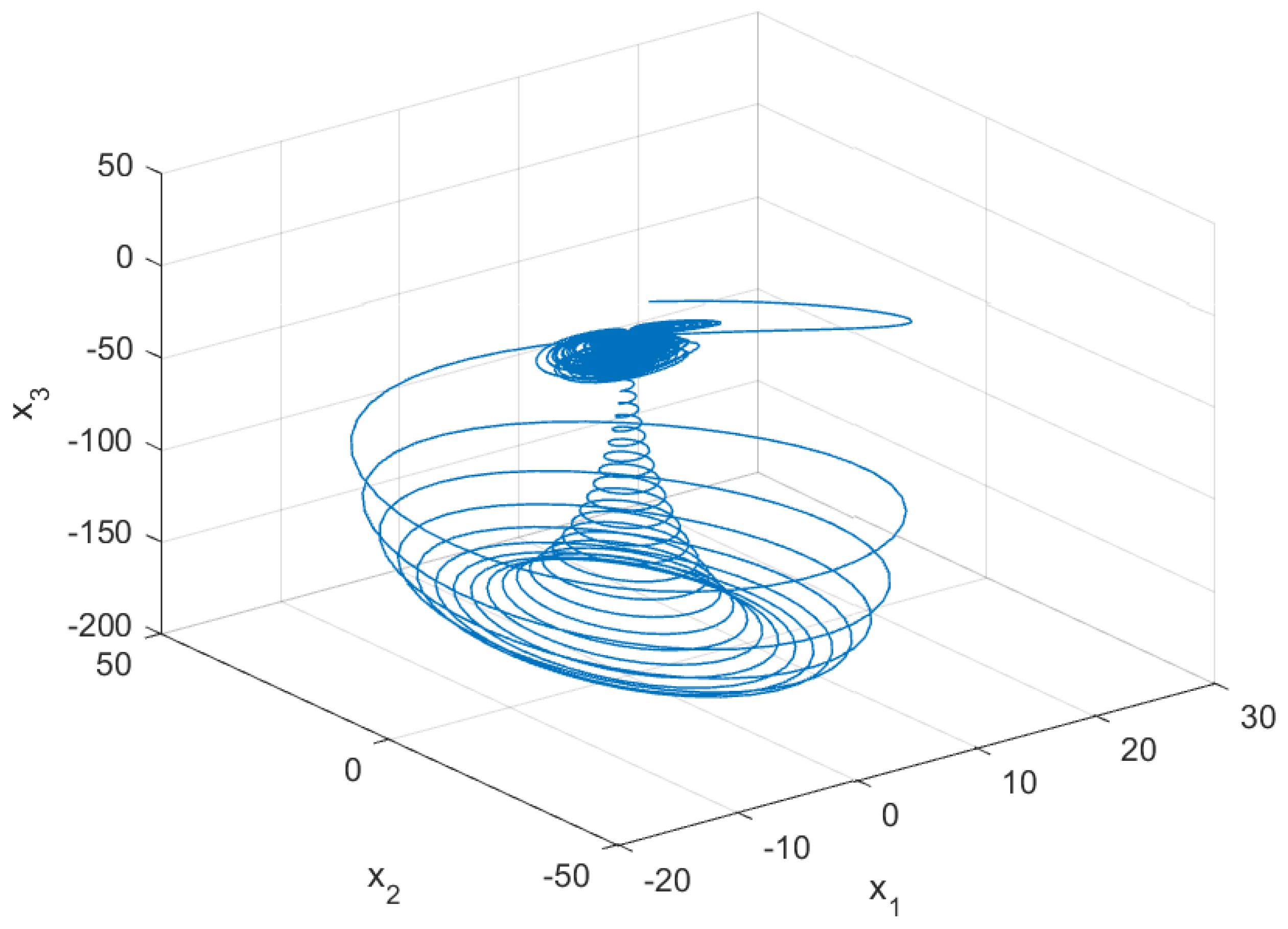
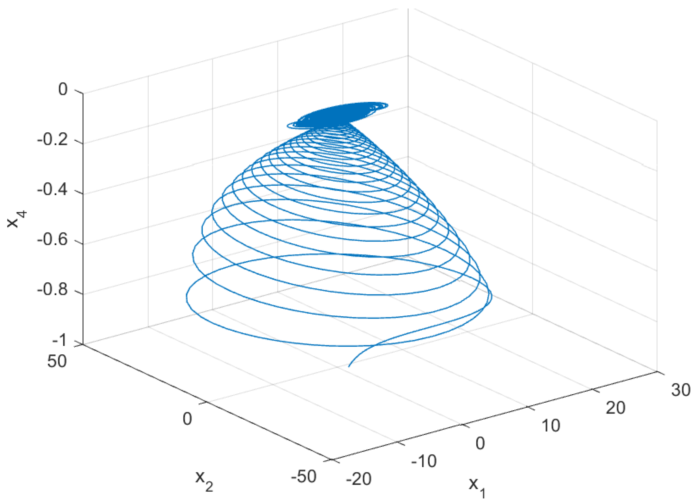
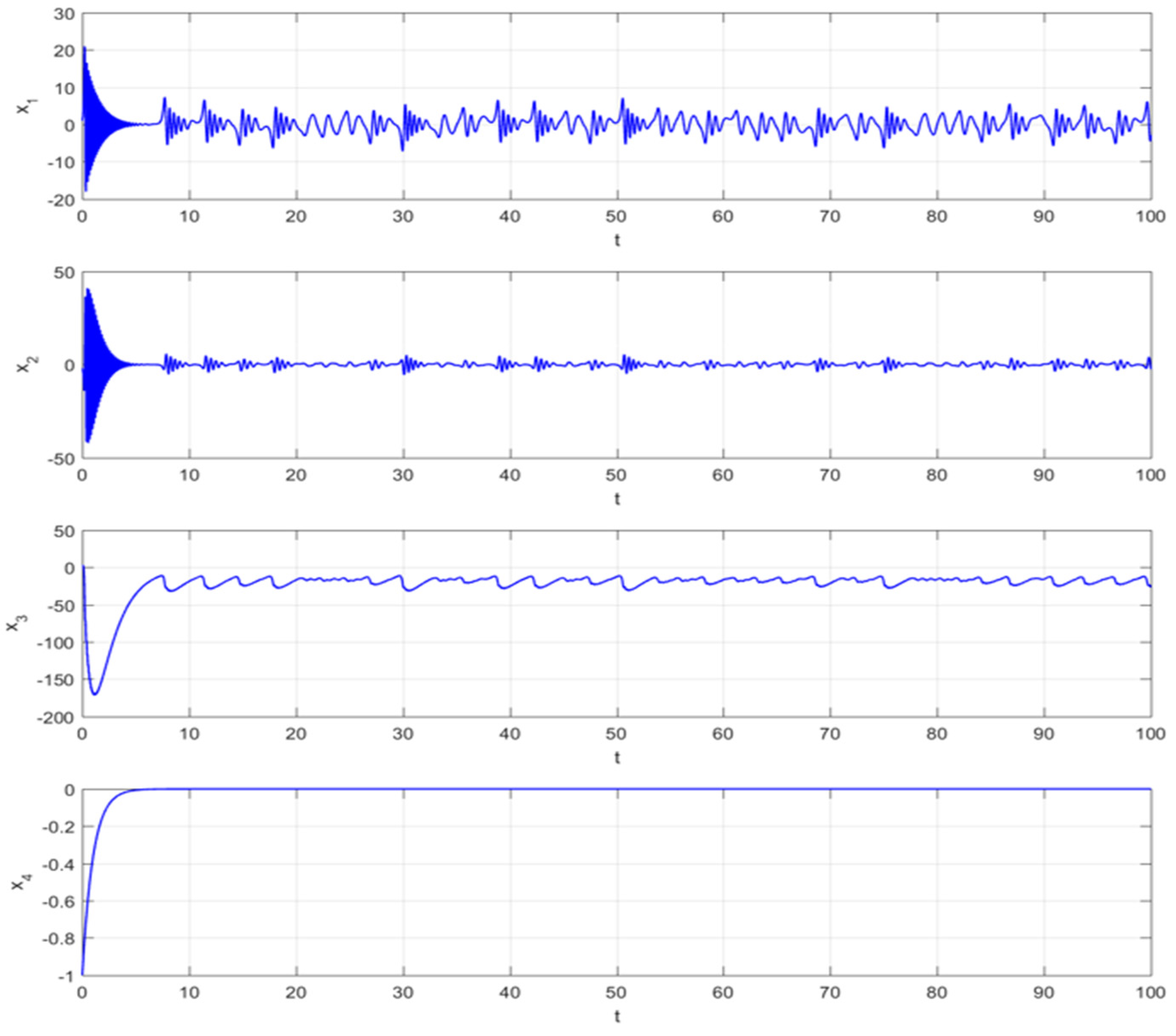
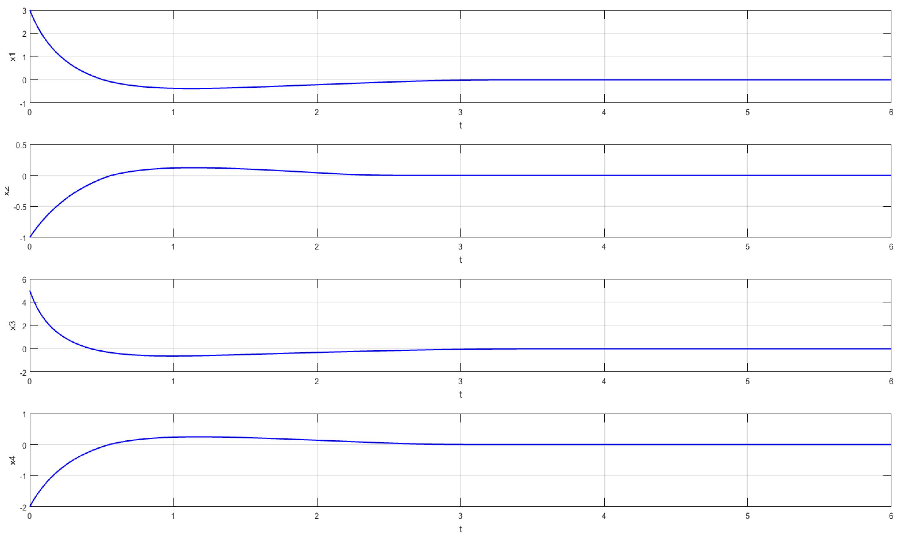
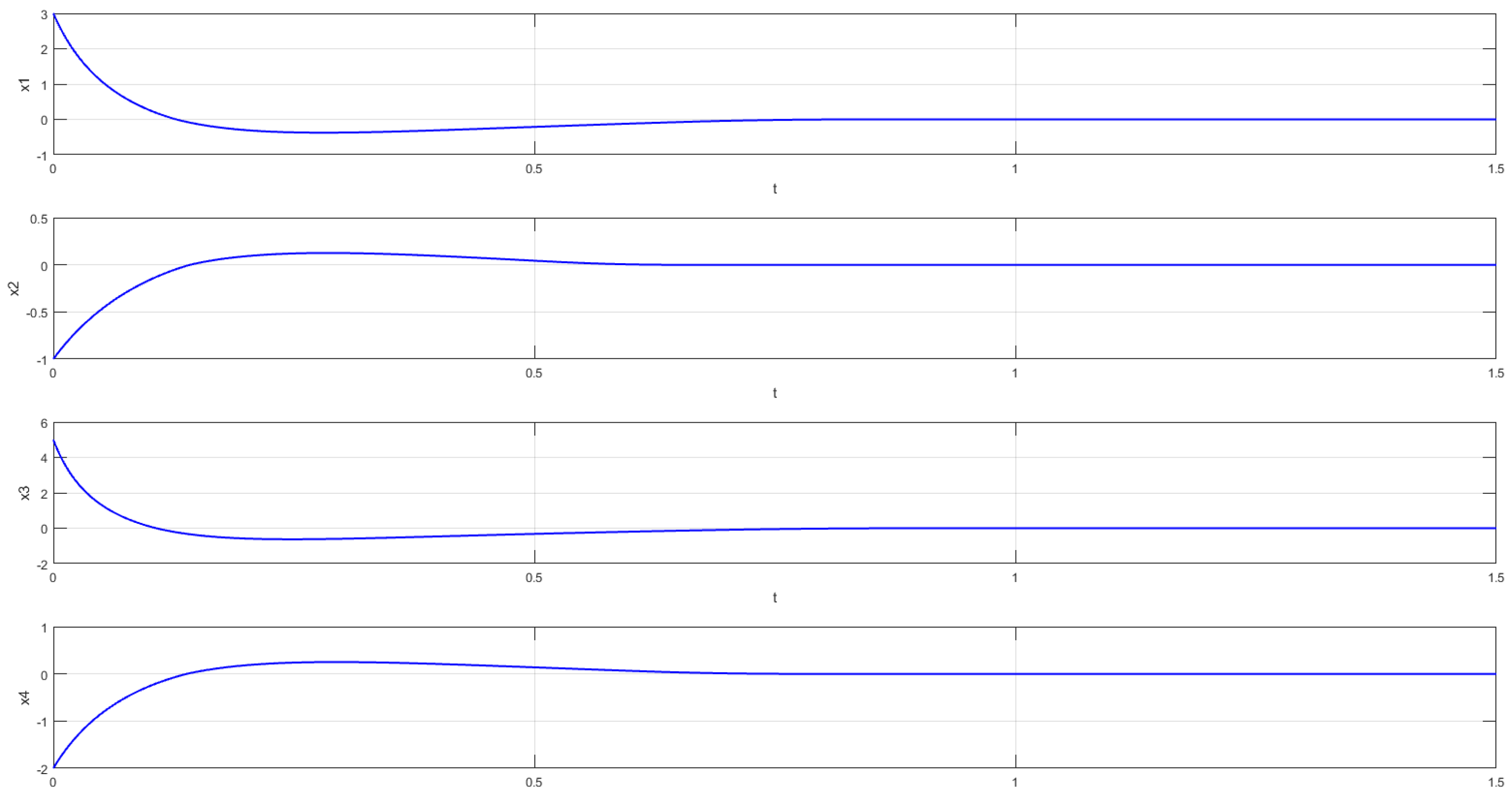
4. Numerical Simulations

To illustrate the performance of the proposed approach, we carried out some numerical simulations of two systems: the PMSM system and the Matouk systems.
Example 1. 
Here the PMSM system is examined from the point of view presented in this article.
The dynamics of the PMSM system are defined as:
x ˙ 1 = x 1 + x 2 x 3 + f 1 x + δ 1 t + u 1 ( t ) x ˙ 2 = x 2 + x 1 x 3 + a 1 x 3 + f 2 x + δ 2 t + u 2 ( t ) x ˙ 1 = a 2 ( x 2 x 3 ) + f 1 x + δ 1 t + u 1 ( t )
where a 1 ,   a 2 are the system’s parameters.
The dynamics of (20) have been investigated in [42,43]. Particularly, system (20) can exhibit chaotic behavior without control, uncertainties, or disturbances, with parameters that are determined by equations a 1 = 20 ,   a 2 = 5.46 . The chaos movement of (20) with x 0 = ( 4.3 ,   5.7 ,   2.7 ) is illustrated in Figure 3. The trajectories of (20) are plotted in Figure 4.
The chaotic system is controlled by (13) that x 0 = ( 4 , 2 , 8 ) , f 1 x = 1.5 sin x 2 ,   f 2 x = 2 c o s x 1 ,   f 3 x = 2.5 sin x 1 c o s ( x 3 ) are the uncertainties, δ 1 t = 1 + 2 s i n ( t ) ,   δ 2 t = 2 sin 3 t cos t ,   δ 3 t = 1.5 + cos ( 3 t ) are the disturbances, u 1 t ,   u 2 t ,   u 3 t are the controllers. We plan the robust controllers according to the results which are discussed.
Remark 4: 
The numerical simulations show that the proposed approach is more efficient that the method proposed in [34]. The trajectories of the controlled system are shown in Figure 5.
Table 1 shows that in our method, x 1 , x 2 ,   a n d   x 3 converge to zero in less than 0.4 s. However, in the method proposed in [34], the convergence occurs after 1 s.
Example 2. 
The controlled Matouk system with internal uncertainties and external disturbances is defined as below:
x ˙ 1 = b 1 x 4 x 2 + b 2 x 1 x 1 x 4 + f 1 x + δ 1 t + u 1 t , x ˙ 2 = b 3 x 1 x 1 x 3 + x 4 + f 2 x + δ 2 t + u 2 t ,                                   x ˙ 3 = b 4 x 3 + b 2 x 1 2 + f 3 x + δ 3 t + u 3 t ,                                               x ˙ 4 = b 5 x 4 + f 4 x + δ 4 t + u 4 t ,
For i 1,2 , 3 , 4 , x i is the state vector, f i x is internal uncertainty, and δ i t is external disturbance. b 1 ,   b 2 ,   b 3 ,   b 4 ,   b 5 are parameters of the system. Let b 1 = 15 ,   b 2 = 2 ,   b 3 = 15 ,   b 4 = 0.5 ,   b 5 = 1 and x 1 0 = 1 ,   x 2 0 = 2 ,   x 3 0 = 3 ,   x 4 0 = 1 . The Matouk system exhibits chaotic behavior without control, uncertainties, or compound disturbances. Its chaotic behavior is shown in Figure 6, Figure 7 and Figure 8. The state trajectories of the system (21).
To stabilize the Matouk system, the internal uncertainties are: f 1 x = 1.5 s i n x 2 ,   f 2 x = 2 c o s x 1 ,   f 3 x = 2.5 s i n x 1 c o s x 3 ,   f 4 x = c o s x 4 , and the external disturbances are assumed as: δ 1 t = 2 cos 2 t sin t + 1 ,   δ 2 t = 2 cos t sin 3 t ,   δ 3 t = cos 3 t + 1.5 ,   δ 4 t = cos 3 t and x 0 = ( 3 , 1 , 5 , 2 ) . The control parameter is K = 0.5 . The novel sliding surface and the robust controllers are defined in (10) and (13). The numerical simulations are shown in Figure 9 and Figure 10.
The actual convergence time is about t 4 for K = 0.25 ; however, for K = 0.25 , T is given by T 4 π seconds.
The actual convergence time is about t 0.9 for K = 2 ; however; T is given by T π 2 . Thus, combining two cases, one can find that t < T which shows the correctness and validity of the derived results.

5. Conclusions

This paper proposed a technique for the fixed-time control of chaotic systems with uncertainties and perturbations. At first, an innovative nonlinear dynamic system is presented which reveals the existence of fixed-time stability. Then, based on this important result, in the form of two theorems, a novel nonlinear terminal sliding mode surface is defined. Afterwards, an appropriate controller is designed. The approach is assessed using a numerical simulation of the PMSM system, and the Matouk system. The obtained results proved the effectiveness of the proposed approach. The proposed method for estimating fixed-time stability can easily be applied to control other chaotic systems with uncertainty and perturbation.

Author Contributions

Conceptualization, A.R., S.M. and A.F.; formal analysis, A.R., S.M. and M.R.G.; funding acquisition, A.F. and A.Z.; investigation, A.R., S.M. and A.Z.; methodology, A.R., S.M. and A.F.; writing—original draft, A.R., S.M. and M.R.G.; writing—review and editing M.R.G., A.F. and A.Z.; supervision, S.M., M.R.G. and A.Z. All authors have read and agreed to the published version of the manuscript.

Funding

The research is partially funded by the Ministry of Science and Higher Education of the Russian Federation as part of the World-class Research Center program: Advanced Digital Technologies (contract No. 075-15-2022-312 dated 20 April 2022).

Institutional Review Board Statement

Not applicable.

Informed Consent Statement

Not applicable.

Data Availability Statement

The data that support the findings of this research paper are available from the corresponding author upon reasonable request.

Conflicts of Interest

The authors declare no conflict of interest.

References

  1. Mirrezapour, S.Z.; Zare, A.; Hallaji, M. A new fractional sliding mode controller based on nonlinear fractional-order proportional integral derivative controller structure to synchronize fractional-order chaotic systems with uncertainty and disturbances. J. Vib. Control 2022, 28, 773–785. [Google Scholar] [CrossRef]
  2. Jiang, X.; Xu, X.; Liang, C.; Liu, H.; Atindana, A.V. Robust controller design of a semi-active quasi-zero stiffness air suspension based on polynomial chaos expansion. J. Vib. Control 2023, 10775463231153706. [Google Scholar] [CrossRef]
  3. Xie, Z.; Sun, J.; Tang, Y.; Tang, X.; Simpson, O.; Sun, Y. A K-SVD Based Compressive Sensing Method for Visual Chaotic Image Encryption. Mathematics 2023, 11, 1658. [Google Scholar] [CrossRef]
  4. Sheng, Z.; Li, C.; Gao, Y.; Li, Z.; Chai, L. A Switchable Chaotic Oscillator with Multiscale Amplitude/Frequency Control. Mathematics 2023, 11, 618. [Google Scholar] [CrossRef]
  5. May, R.M. Deterministic models with chaotic dynamics. Nature 1975, 256, 165–166. [Google Scholar] [CrossRef]
  6. Ott, E.; Grebogi, C.; Yorke, J.A. Controlling chaos. Phys. Rev. Lett. 1990, 64, 1196–1199. [Google Scholar] [CrossRef]
  7. Pecora, L.M.; Carroll, T.L. Synchronization in chaotic systems. Phys. Rev. Lett. 1990, 64, 821–824. [Google Scholar] [CrossRef]
  8. Lin, W.; Qian, C. Adding one power integrator: A tool for global stabilization of high-order lower-triangular systems. Syst. Control. Lett. 2000, 39, 339–351. [Google Scholar] [CrossRef]
  9. Bernstein, S.P.; Bernstein, D.S. Finite-Time Stability of Continuous Autonomous Systems. SIAM J. Control. Optim. 2000, 38, 751–766. [Google Scholar]
  10. Aghababa, M.P.; Khanmohammadi, S.; Alizadeh, G. Finite-time synchronization of two different chaotic systems with unknown parameters via sliding mode technique. Appl. Math. Model. 2011, 35, 3080–3091. [Google Scholar] [CrossRef]
  11. Polyakov, A. Nonlinear Feedback Design for Fixed-Time Stabilization of Linear Control Systems. IEEE Trans. Autom. Control 2012, 57, 2106–2110. [Google Scholar] [CrossRef] [Green Version]
  12. Polyakov, A.; Efimov, D.; Perruquetti, W. Finite-time and fixed-time stabilization: Implicit Lyapunov function approach. Automatica 2015, 51, 332–340. [Google Scholar] [CrossRef] [Green Version]
  13. Luo, R.; Zeng, Y. The control of chaotic systems with unknown parameters and external disturbance via backstepping-like scheme. Complexity 2016, 21, 573–583. [Google Scholar] [CrossRef]
  14. Shi, K.; Tang, Y.; Liu, X.; Zhong, S. Non-fragile sampled-data robust synchronization of uncertain delayed chaotic Lurie systems with randomly occurring controller gain fluctuation. ISA Trans. 2017, 66, 185–199. [Google Scholar] [CrossRef]
  15. Luo, R.; Su, H. Finite-time control and synchronization of a class of systems via the twisting controller. Chin. J. Phys. 2017, 55, 2199–2207. [Google Scholar] [CrossRef]
  16. Zhang, T.; Xia, M.; Yi, Y. Adaptive neural dynamic surface control of strict-feedback nonlinear systems with full state constraints and unmodeled dynamics. Automatica 2017, 81, 232–239. [Google Scholar] [CrossRef]
  17. Nafia, N.; El Kari, A.; Ayad, H.; Mjahed, M. Robust Interval Type-2 Fuzzy Sliding Mode Control Design for Robot Manipulators. Robotics 2018, 7, 40. [Google Scholar] [CrossRef] [Green Version]
  18. Matouk, A.E. Dynamics and control in a novel hyperchaotic system. Int. J. Dyn. Control 2019, 7, 241–255. [Google Scholar] [CrossRef]
  19. Kim, Y.; Oh, T.H.; Park, T.; Lee, J.M. Backstepping control integrated with Lyapunov-based model predictive control. J. Process Control 2019, 73, 137–146. [Google Scholar] [CrossRef]
  20. Rabiee, H.; Ataei, M.; Ekramian, M. Continuous nonsingular terminal sliding mode control based on adaptive sliding mode disturbance observer for uncertain nonlinear systems. Automatica 2019, 109, 108515. [Google Scholar] [CrossRef]
  21. Runzi, L.; Huang, M.; Su, H. Robust Control and Synchronization of 3-D Uncertain Fractional-Order Chaotic Systems with External Disturbances via Adding One Power Integrator Control. Complexity 2019, 2019, 8417536. [Google Scholar]
  22. Ma, H.; Liang, H.; Zhou, Q.; Ahn, C.K. Adaptive Dynamic Surface Control Design for Uncertain Nonlinear Strict-Feedback Systems With Unknown Control Direction and Disturbances. IEEE Trans. Syst. Man Cybern. Syst. 2019, 49, 506–515. [Google Scholar] [CrossRef]
  23. Li, Z.W. Fixed-Time and Finite-Time Synchronization for a Class of Output-Coupling Complex Networks via Continuous Control. Int. J. Commun. Netw. Syst. Sci. 2019, 12, 151–169. [Google Scholar] [CrossRef] [Green Version]
  24. Yin, X.; She, J.; Liu, Z.; Wu, M.; Kaynak, O. Chaos suppression in speed control for permanent-magnet-synchronous-motor drive system. J. Frankl. Inst. 2020, 357, 13283–13303. [Google Scholar] [CrossRef]
  25. Rashidnejad, Z.; Karimaghaee, P. Synchronization of a class of uncertain chaotic systems utilizing a new finite-time fractional adaptive sliding mode control. Chaos Solitons Fractals X 2020, 5, 100042. [Google Scholar] [CrossRef]
  26. Chen, C.; Li, L.; Peng, H.; Yang, Y.; Mi, L.; Zhao, H. A new fixed-time stability theorem and its application to the fixed-time synchronization of neural networks. Neural Netw. 2020, 123, 412–419. [Google Scholar] [CrossRef]
  27. Su, H.; Luo, R.; Fu, J.; Huang, M. Fixed time stability of a class of chaotic systems with disturbances by using sliding mode control. ISA Trans. 2021, 118, 75–82. [Google Scholar] [CrossRef] [PubMed]
  28. Tong, D.; Xu, C.; Chen, Q.; Zhou, W. Sliding mode control of a class of nonlinear systems. J. Frankl. Inst. 2020, 357, 1560–1581. [Google Scholar] [CrossRef]
  29. Xiong, X.; Yang, X.; Cao, J.; Tang, R. Finite-time control for a class of hybrid systems via quantized intermittent control. Sci. China Inf. Sci. 2020, 63, 192201. [Google Scholar] [CrossRef]
  30. Shi, K.; Jun, w.; Zhong, S.; Tang, Y.; Cheng, J. Hybrid-driven finite-time H∞ sampling synchronization control for coupling memory complex networks with stochastic cyber attacks. Neurocomputing 2020, 387, 241–254. [Google Scholar] [CrossRef]
  31. Hua, L.; Zhong, S.; Shi, K.; Zhang, X. Further results on finite-time synchronization of delayed inertial memristive neural networks via a novel analysis method. Neural Netw. 2020, 127, 47–57. [Google Scholar] [CrossRef] [PubMed]
  32. He, X.; Li, X.; Nieto, J.J. Finite-time stability and stabilization for time-varying systems. Chaos Solitons Fractals 2021, 148, 111076. [Google Scholar] [CrossRef]
  33. Chen, Y.; Li, X.; Liu, S. Finite-time stability of ABC type fractional delay difference equations. Chaos Solitons Fractals 2021, 152, 111430. [Google Scholar] [CrossRef]
  34. Su, H.; Luo, R.; Huang, M.; Fu, J. Robust Fixed Time Control of a Class of Chaotic Systems with Bounded Uncertainties and Disturbances. Int. J. Control. Autom. Syst. 2022, 20, 813–822. [Google Scholar] [CrossRef]
  35. Kavikumar, R.; Kaviarasan, B.; Lee, Y.-G.; Kwon, O.-M.; Sakthivel, R.; Choi, S.-G. Robust dynamic sliding mode control design for interval type-2 fuzzy systems. Discret. Contin. Dyn. Syst. S 2022, 15, 1839–1858. [Google Scholar] [CrossRef]
  36. Luo, D.; Tian, M.; Zhu, Q. Some results on finite-time stability of stochastic fractional-order delay differential equations. Chaos Solitons Fractals 2022, 158, 111996. [Google Scholar] [CrossRef]
  37. He, X.; Li, X.; Song, S. Finite-time stability of state-dependent delayed systems and application to coupled neural networks. Neural Netw. 2022, 154, 303–309. [Google Scholar] [CrossRef] [PubMed]
  38. Gokul, P.; Rakkiyappan, R. New finite-time stability for fractional-order time-varying time-delay linear systems: A Lyapunov approach. J. Frankl. Inst. 2022, 359, 7620–7631. [Google Scholar]
  39. Long, S.; Zhou, L.; Zhong, S.; Liao, D. An improved result for the finite-time stability of the singular system with time delay. J. Frankl. Inst. 2022, 359, 9006–9021. [Google Scholar] [CrossRef]
  40. Yuan, Y.; Zhao, J.; Sun, Z.-Y. Fast finite time stability of stochastic nonlinear systems. J. Frankl. Inst. 2022, 359, 9039–9055. [Google Scholar] [CrossRef]
  41. Michalak, A. Finite-time and fixed-time stability analysis for time-varying systems: A dual approach. J. Frankl. Inst. 2022, 359, 10676–10687. [Google Scholar] [CrossRef]
  42. Liu, J.X.; Wang, Z.X.; Lei, T.F.; Yin, W.J. Finite-time chaotic synchronization control of permanent magnet synchronous motor. Small Spec. Electr. Mach. 2019, 47, 45–53. [Google Scholar]
  43. Yang, X.H.; Liu, X.P.; Hu, L.L.; Xu, S.P. Robust sliding mode mariable structure synchronization control of chaos in permanent magnet synchronous motor. Modul. Mach. Tool Autom. Manuf. Tech. 2012, 8, 93–95. [Google Scholar]
Figure 1. Graph of x ( t ) when K = 2 ,   x 0 = 7 .
Mathematics 11 03273 g001
Figure 2. Graph of x ( t ) when K = 1 2 , x 0 = 3 .
Mathematics 11 03273 g002
Figure 3. The chaotic attractor of (20) with x 0 = ( 4.3,5.7 ,   2.7 ) .
Mathematics 11 03273 g003
Figure 4. The state trajectories of system (20).
Mathematics 11 03273 g004
Figure 5. Trajectories of the controlled system with K = 0.25 according to controller in our method and the method suggested in [34].
Mathematics 11 03273 g005
Figure 6. The chaotic attractor of (21).
Mathematics 11 03273 g006
Figure 7. The chaotic attractor of (21).
Mathematics 11 03273 g007
Figure 8. The state trajectories of the system (21).
Mathematics 11 03273 g008
Figure 9. The states x 1 , x 2 , x 3 , x 4 of (21) with K = 0.25 .
Mathematics 11 03273 g009
Figure 10. The states x 1 , x 2 , x 3 , x 4 of (21) with K = 2 .
Mathematics 11 03273 g010
Table 1. Performance comparison.
MethodTime (s)00.20.40.60.81
Our method x 1 −40.1638−3.9031 × 10⁻¹⁸−3.9031 × 10⁻¹⁸−3.9031 × 10⁻¹⁸−3.9031 × 10−18
x 2 2−0.06521.0503 × 10−191.0503 × 10−191.0503 × 10−191.0503 × 10⁻¹⁹
8−0.26884.5794 × 10−174.5794 × 10−174.5794 × 10−174.5794 × 10⁻¹⁷
Method of Ref [34] x 1 −40.39750.05250.002−2.4926 × 10⁻⁴−2.6047 × 10−5
x 2 2−0.2800−0.0507−1.8392 × 10−41.4824 × 10−52.0169 × 10−5
x 3 8−0.6131−0.1117−0.0031−1.4171 × 10−41.7504 × 10−4
Disclaimer/Publisher’s Note: The statements, opinions and data contained in all publications are solely those of the individual author(s) and contributor(s) and not of MDPI and/or the editor(s). MDPI and/or the editor(s) disclaim responsibility for any injury to people or property resulting from any ideas, methods, instructions or products referred to in the content.

