Article

On Surprise Indices Related to Univariate Discrete and Continuous Distributions: A Survey

by
Indranil Ghosh
* and
Tamara D. H. Cooper
Department of Mathematics and Statistics, University of North Carolina, Wilmington, NC 28403, USA
*
Author to whom correspondence should be addressed.
Mathematics 2023, 11(14), 3234; https://doi.org/10.3390/math11143234
Submission received: 21 June 2023 / Revised: 15 July 2023 / Accepted: 17 July 2023 / Published: 23 July 2023
(This article belongs to the Special Issue Parametric and Nonparametric Statistics: From Theory to Applications)

Abstract

:
The notion that the occurrence of an event is surprising has been discussed in the literature without adequate details. By definition, a surprise index is an index by which how surprising an event is may be determined. Since its inception, this index has been evaluated for univariate discrete probability models, such as the binomial, negative binomial, and Poisson probability distributions. In this article, we derive and discuss using numerical studies, in addition to the above-mentioned probability models, surprise indices for several other univariate discrete probability models, such as the zero-truncated Poisson, geometric, Hermite, and Skellam distributions, by adopting a established strategy and using the Mathematica, version 12 software. In addition, we provide symbolical expressions for the surprise index for several univariate continuous probability models, which has not been previously discussed. For illustrative purposes, we present some possible real-life applications of this index and potential challenges to extending the notion of the surprise index to bivariate and higher dimensions, which might involve ubiquitous normalizing constants.

1. Introduction

The notion of the surprise index (SI) is not new in the literature, but has not been discussed thoroughly due to a lack of applicability and complexity in deriving for probability models that do not conform to well-known generating functions. The scarcity of scholarly works in this direction is reminiscent of this fact. The earliest reference dates back to 1948, when [1] asserted that an event with a low probability may be rare but is not surprising.
Interestingly enough, research on this topic is very limited. Some pertinent references are given as follows: Ref. [2] generalized and derived the SI for the multivariate normal distribution, but it has a different expression and notion. Ref. [3] derived the SIs for the binomial and Poisson distributions but without adequate details. Ref. [4] discussed the SI for the negative binomial distribution. Ref. [5] discussed the role of the SI in the context of macro-surprises from a monetary economics perspective. From the above-cited references, one may arrive at the conclusion that finding the SI is difficult to achieve analytically and subsequently requires the assistance of a powerful and efficient computing environment, such as Mathematica, which is utilized in this paper to obtain closed-form expressions for probability distributions in both the discrete domain and in the continuous domain other than those that have already been discussed.
In this article, we aim to discuss, in adequate details, the computation of SIs for various discrete probability distributions, including the binomial, negative binomial, and Poisson distributions (i.e., those that have been at least discussed in the literature), and SIs for zero-truncated Poisson, geometric, Hermite, and Skellam distributions, which are new contributions to the current topic. In addition, we also provide an analogous expression for deriving the SI for univariate continuous probability models using the definition given in Equation (19) and defined later. For illustrative purposes, we compute SIs for various well-known univariate absolutely continuous probability models using Equation (19). It appears that, in most of the cases, the resulting expression of the SI associated with each of the discrete probability distributions is available in closed form, involving special functions and infinite series wherever applicable. Furthermore, we provide some empirical studies of the SIs corresponding to several discrete probability models. We conjecture that a similar development can be made in terms of identifying SIs for bivariate and/or multivariate continuous probability models, which will be the subject matter of a separate article. In summary, the major contributions of this article on the topic of SIs can be summarized as follows:
  • We revisit the computation of the SIs for the binomial, Poisson, and negative binomial distributions and provide the correct expression of the SI for the Poisson distribution using Mathematica.
  • Surprise indices are computed for the geometric and negative binomial, zero-truncated Poisson, and Hermite (for which closed-form expressions involving special functions and/or infinite series are available) distributions, while for the generalized Poisson distribution, the associated SI is not available in closed form, and a numerical solution is to be searched for. All of these derivations are new contributions to this topic.
  • In addition, we provide the derivation of SIs for univariate continuous probability models using an analogous expression based on the geometric mean of a random variable.
  • Finally, we conduct empirical studies on SIs for several of the discrete distributions with varying parameter choices, and several useful observations are derived accordingly.
The remainder of this article is organized in the following manner: In Section 2, we provide the computational details of deriving the SI for each of the univariate discrete probability models assumed in this paper with empirical studies on several of such probability models. In Section 3, we derive the SI for a continuous probability model based on the definition according to [2] and provide some useful conjectures on the properties of SIs. Section 4 presents several potential applications of the SI in a practical setting along with some potential challenges to extending this definition in bivariate and higher domains. Finally, some concluding remarks are presented in Section 5.

2. Surprise Index Derivation: Preliminaries

We begin this section by providing the definition of SI. According to [1], the SI, S i , is defined as the comparison of the expected probability and the observed probability, which has the following form:
S i = p m 2 p i ,
where p m = P X = m and p i represents the probability that an event E i has actually occurred. The expression in Equation (1) of the SI is from [3]. This feature can be obtained for discrete probability distributions in computing their corresponding probability generating functions, a strategy which is discussed later. Based on a suggestion by an anonymous reviewer, alternatively, Equation (1) can be rewritten as
S i = E ( p X ) p i .
Noticeably, this form is also independently obtained in [1].
Next, we revisit the computation of the SIs for the binomial, negative binomial, and Poisson distributions that have been independently discussed and derived in [3,4]. Proceeding in the same manner, we derive SIs for the zero-truncated Poisson, geometric, Hermite, and Skellam distributions. The process of obtaining the SI involves the following steps (for details, see [3]):
  • Step 1: Calculate the generating function of p m , which is of the form m 0 p m x m from a given probability mass function (p.m.f.).
  • Step 2: Set x = e i θ , and e i θ , to obtain the following quantity m 0 p m 2 = m 0 p m e i m θ p m e i m θ , which is the numerator of Equation (1), where i = 1 .
  • Step 3: Integrate the simplified quantity on the R.H.S. obtained in Step 2, from 0 to 2 π .
Then, substitute the value obtained in Step 3 to the numerator of Equation (1). Observe that, since the rationale behind this strategy of obtaining the SI has already been discussed in [3], it is not discussed here.
Next, this simple process is carried out below, for each of the discrete probability distributions selected for this purpose. It is important to note that the goal of the above steps is to obtain an expression for the sum of p m 2 , which involves solving the integral in step 3. In the next subsection, we begin by revisiting the SI for a binomial distribution at first.

2.1. Surprise Index for a Binomial Distribution

The binomial distribution is denoted as B ( n , p ) , with n { 0 , 1 , 2 , } being the number of trials and p [ 0 , 1 ] being the probability of success resulting from each trial. The associated probability mass function (p.m.f.) is
p m = n m p m q n m ,
where m { 0 , 1 , 2 , , n } is the number of successes, with p + q = 1 . The associated generating function will be
m = 0 n p m x m = q + p x n .
Then, following steps two and three (given earlier) and simplifying, we obtain
m = 0 n p m 2 = m = 0 n p m exp ( i m θ ) p m exp ( i m θ ) = 1 2 π 0 2 π ( q 2 + 2 q p cos ( θ ) + p 2 ) n d θ = p q 2 n 2 F 1 1 2 , n ; 1 ; 4 p q ( p q ) 2 , on using Mathematica ,
where
2 F 1 a , b ; c , d = ( a ) n ( b ) n d n n ! ( c ) n ,
is the Gauss hypergeometric function, and ( W ) n = W ( W + 1 ) ( W + 2 ) ( W + n 1 ) if n > 0 and ( W ) n = 1 if n = 0 .
Therefore, the SI for the binomial distribution related to the i-th probability is (on substituting Equation (2) in the numerator of Equation (1)):
S i = ( p q ) 2 n 2 F 1 1 2 , n ; 1 ; 4 p q ( p q ) 2 p i .
For illustrative purposes, we assume some representative values of p and subsequently compute the associated values of S i for a fixed value of n = 10 and for varying choices m, p, and q in Equation (3), which are reported in Table 1.
From Table 1, we can observe the following:
  • For fixed n , with p i decreasing, the corresponding SI values increase, which is expected.
  • For fixed values of p and q , as the number of successes increase and with p i decreasing, the SI values increase.

2.2. Surprise Index for a Negative Binomial Distribution

The negative binomial distribution is denoted as N B ( r , p ) , with r > 0 as the number of successes until the experiment is terminated and p [ 0 , 1 ] being the probability of success for each experiment. The associated p.m.f. is
p m = m + r 1 m p r q m ,
where m { 0 , 1 , 2 , } is the number of failures. Consequently, the generating function will be
p m x m = p 1 q x r .
Proceeding as before, we obtain
m = 0 n p m 2 = 1 2 π 0 2 π p 2 ( q 2 2 q cos ( θ ) + 1 ) r d θ = p 2 ( q + 1 ) 2 r 2 F 1 1 2 , r ; 1 ; 4 q ( q + 1 ) 2 ,
using Mathematica, where 2 F 1 ( ) is defined in Equation (3).
Thus, the SI for the negative binomial distribution is, on substituting Equation (5) in the numerator of Equation (1),
S i = p 2 ( q + 1 ) 2 r 2 F 1 1 2 , r ; 1 ; 4 q ( q + 1 ) 2 p i .
Assuming several representative values of p and q , and substituting various values for r and p i in Equation (6), we find the following values of S i for this distribution, which are presented in Table 2.
From Table 2, one may observe the following:
  • The SI values are dependent on the magnitude of either or both of p and p i .
  • For fixed p , q as p i increases, the SI values decrease for varying r , m .
  • For r > m , p < q , with q increasing, the SI value increases.
  • For r < m , with p < q , and q decreasing, as m decreases, the SI values increase.

2.3. Surprise Index for a Poisson Distribution

The associated p.m.f. is
p m = λ m e λ m ! ,
where m { 0 , 1 , 2 , } is the number of occurrences and λ ( 0 , ) . The associated generating function is
m 0 p m x m = e λ e λ x .
Proceeding as before,
m = 0 n p m 2 = e 2 λ 2 π 0 2 π e 2 λ cos ( θ ) d θ = e 2 λ I 0 ( 2 λ ) ,
where I 0 ( ) is the zero-order modified Bessel function of the first kind.
Therefore, the SI for the Poisson distribution on substituting Equation (7) in the numerator of Equation (1) is
S i = e 2 λ I 0 ( 2 λ ) p i .
Substituting various values for λ and m in Equation (8), we find the following values of S i for this distribution, given in Table 3.
From Table 3, it appears that
  • For a fixed λ , with m increasing and p i decreasing, the SI values increase.
  • For a fixed m , with λ increasing, the SI values decrease.
For a comprehensive view of the SI in this case, further empirical studies are required.

2.4. Surprise Index for a Zero-Truncated Poisson Distribution

The zero-truncated Poisson distribution is denoted as ZTP ( λ ) with parameter λ ( 0 , ) . The p.m.f. is
p m = e λ λ m m ! 1 e λ = λ m ( e λ 1 ) m ! ,
where m { 1 , 2 , 3 , } is the number of occurrences; for a detailed study on this distribution, see [6]. The associated generating function will be
m = 1 p m x m = e λ x e λ 1 .
Proceeding as before, the numerator of Equation (1) in this case, will be
m = 0 p m 2 = 1 2 π ( e 2 λ 2 e λ + 1 ) 0 2 π e 2 λ cos ( θ ) d θ = ( e 2 λ 2 e λ + 1 ) 1 I 0 ( 2 λ ) ,
where I 0 ( ) has been defined earlier in the previous subsection. Therefore, upon substituting Equation (9) in the numerator of Equation (1), the SI for the zero-truncated Poisson distribution will be
S i = ( e 2 λ 2 e λ + 1 ) 1 I 0 ( 2 λ ) p i .
Substituting various representative values for λ and m in Equation (10), we find the following values of S i for this distribution, which is presented in Table 4.
From Table 4, one can observe the following:
  • The SI values are slightly different from the Poisson distribution’s SI values. Also, we see that smaller values of λ generate greater differences between the zero-truncated Poisson and the Poisson SI values.
  • The behavior/changing pattern of the SI values are exactly the same (except for the magnitude) as in the previous case (Poisson distribution), for varying choices of λ , m and p i .

2.5. Surprise Index for a Geometric Distribution

The geometric distribution is denoted as Geo ( p ) , with p { 1 , 2 , 3 , } being the number of Bernoulli trials needed to achieve one success. The associated p.m.f. is
p m = ( 1 p ) m 1 p = p q m 1 ,
where m { 1 , 2 , 3 , } is the number of successes. The generating function is then found to be
p m x m = p x 1 q x .
Consequently, the numerator of Equation (1) will be
m = 0 p m 2 = p 2 2 q 2 π 0 2 π ( q 2 2 q cos ( θ ) + 1 ) 1 d θ = p 2 q 2 1 q 2 ,
on using Mathematica.
Hence, on substituting Equation (11) in the numerator of Equation (1), we have the following expression for the SI for the geometric distribution:
S i = p 2 p i q 2 1 q 2 .
Assuming various representative values for m and p , in Equation (12), we find the following values of S i for this distribution, which are given in Table 5.
From Table 5, one may observe the following:
  • For fixed p , q with p < q and with m increasing, the SI values exhibit an increasing pattern.
  • For fixed m , with q decreasing, the SI values increase.

2.6. Surprise Index for a Hermite Distribution

The Hermite distribution is denoted as Herm a 1 , a 2 with parameters a 1 0 and a 2 0 . This distribution is used to measure count data using more than one parameter and has been used in biological research. There are several scholarly studies related to this distribution that exist in the literature. For example, Ref. [7] discussed several useful structural properties of the Hermite distribution and they established the fact that this distribution is the generalized Poisson distribution. Ref. [8] have discussed the utility of this distribution in the context of a zero-inflated overdispersed probability model. Ref. [9] developed an R package hermite to apply generalized hermite distribution in modeling real-world scenario(s) of fitting count data in the presence of overdispersion or multimodality with a lot more added flexibility in terms of inference under the classical method. The associated p.m.f. of the random variable Y = X 1 + X 2 is
p m = e ( a 1 + a 2 ) j = 0 m / 2 a 1 m 2 j a 2 j ( m 2 j ) ! j ! .
where m = 0 , 1 , 2 , and m / 2 is the integer part of m / 2 , and a 1 , a 2 0 are the parameters associated with the two independent Poisson variables X 1 and X 2 , respectively. The associated generating function is given by
m = 0 m / 2 p m x m = e a 1 ( x 1 ) + a 2 ( x 2 1 ) .
Proceeding as before, the numerator of Equation (1) will be
m = 0 n p m 2 = 1 2 π 0 2 π e 2 a 1 ( c o s ( θ ) 1 ) + 2 a 2 ( c o s ( θ ) 1 ) d θ = 1 2 π j = 0 1 j ! 0 2 π [ 2 a 1 ( c o s ( θ ) 1 ) + 2 a 2 ( c o s ( θ ) 1 ) ] j d θ = j = 0 1 j ! ( a 1 ) j Γ ( 2 j + 1 ) a 1 a 1 + 4 a 2 j 2 F ˜ 1 j , j + 1 2 ; j + 1 ; 4 a 2 a 1 + 4 a 2 Γ ( j + 1 ) ,
where 2 F ˜ 1 ( ) is the regularized hypergeometric distribution, obtained using Mathematica. Therefore, upon substituting Equation (17) in the numerator of Equation (1), the SI for the Hermite distribution will be
S i = j = 0 1 j ! ( a 1 ) j Γ ( 2 j + 1 ) a 1 a 1 + 4 a 2 j 2 F ˜ 1 j , j + 1 2 ; j + 1 ; 4 a 2 a 1 + 4 a 2 p i Γ ( j + 1 ) .
Substituting various values for m ,   a 1 , and   a 2 in Equation (14), one can find values of S i for this distribution, which is not reported in this paper for brevity. Also, it is quite difficult to obtain numerically, as it involves infinite sums and special functions.

2.7. Surprise Index for a Skellam Distribution

The Skellam distribution, also known as the Poisson difference distribution, is derived from the difference of two Poisson random variables (for details, see [10]) and is denoted as Skellam ( μ 1 , μ 2 ) with parameters μ 1 0 and μ 2 0 . This distribution may be used for describing the point spread distribution for sports such as hockey, where all points scored are equal, describing the statistics of the difference of two images with simple photon noise, or studying treatment effects, as discussed in [10]. The p.m.f. when considering two Poisson random variables is given by
p m = e ( μ 1 + μ 2 ) μ 1 μ 2 m / 2 I m ( 2 μ 1 μ 2 ) ,
where m is an integer and I m ( z ) is the m-th order modified Bessel function of the first kind. The associated generating function will be
p m x m = e ( μ 1 + μ 2 ) + μ 1 m + μ 2 / m .
Again, by proceeding as before, the numerator of Equation (1) can be derived using the infinite series expression for the exponential function and using Mathematica,as follows:
m = 0 n p m 2 = 1 2 π 0 2 π e ( 2 μ 1 + 2 μ 2 ) ( c o s ( θ ) 1 ) d θ = 1 2 π j = 0 2 μ 1 + μ 2 j j ! 0 2 π c o s ( θ ) 1 j d θ = j = 0 2 μ 1 + μ 2 j j ! ( 2 ) j Γ j + 1 2 π Γ ( j + 1 ) ,
Subsequently, upon substituting Equation (15) in the numerator of Equation (1), the SI for the Skellam distribution can be written as
S i = j = 0 2 μ 1 + μ 2 j j ! ( 2 ) j Γ j + 1 2 p i π Γ ( j + 1 ) .
Substituting various values for m , μ 1 , and μ 2 in Equation (16), one can find expressions of the SI for this distribution. However, from Equation (16), it is clear that it would be difficult to obtain numerical values as the expression involves infinite sum and gamma functions.

2.8. Surprise Index for a Generalized Poisson Distribution

The generalized Poisson distribution is denoted as GDP   ( θ , λ ) with parameters θ   and   λ ,   0 λ < 1 and   θ > 0 . To allow us to differentiate between the parameter and the integration variable, we change θ to α , and then, the p.m.f. is
p m = α ( α + n λ ) m 1 e m λ α m ! ,
where m { 0 , 1 , 2 , } is the number of occurrences. The associated generating function is then, according to [11],
p m x m = exp α λ W λ x exp [ λ ] + λ ,
where W ( · ) is the Lambert W function. Continuing with the prescribed process, we found the following integral form:
p m 2 = 1 2 π 0 2 π exp α λ W λ exp [ i θ ] exp [ λ ] + W λ exp [ i θ ] exp [ λ ] + 2 λ d θ .
Consequently, the associated SI for a GPD, upon substituting Equation (17) in the numerator of Equation (1), will be
S j = 1 2 π 0 2 π exp α λ W λ exp [ i θ ] exp [ λ ] + W λ exp [ i θ ] exp [ λ ] + 2 λ d θ × α ( α + n λ ) j 1 e i λ α j ! 1 .
Noticeably, from Equation (18), it can be observed that this integral is difficult to solve in order to obtain a closed and analytically tractable form because of the involvement of the Lambert W function which has both real and imaginary parts. Numerical methods must be adopted, which we have not considered for brevity.
In addition, for illustrative purposes, we have also provided graphs of the SI for several discrete probability distributions discussed in this section in Appendix B.

3. Surprise Index for Continuous Probability Models

For a continuous random variable (r.v.), the associated expression for the SI is given by [2] and has the following form:
ζ = E p * | H p ,
where p * is the r.v. that is the probability density function (p.d.f.) of the original r.v., p is a realization of p * , and H is a simple statistical hypothesis. Equivalently, we may rewrite the definition as follows. Let X be a continuous random variable with density function f ( ) . Then, for all x S ( X ) , the SI is given by
S x = E [ f ( X ) ] f ( x ) .
However, an alternative version which does involve the geometric expectation (it is termed as a generalization of the SI) is given by
ζ 0 = G E ( p * ) p = exp E log X p ,
where G E stands for the geometric expectation which will be equivalently evaluated using E ( log X ) . For computation of the SI for various continuous probability models, we use Equation (19). In Table 6, we provide the expression of Equation (19), which can be viewed as an expression of the SI (according to [2]) for various univariate absolute continuous distributions. The symbolic computations are all carried out using Mathematica.
From Table 6, one can make the following observations for fixed X = x :
  • For uniform a , b , and b increasing and a decreasing, the SI will increase.
  • For Beta a , b , as a increases and b increases, SI decreases. On the other hand, when both a and b increase, the SI increases.
  • For Beta (type-II) α , β , when both α , β increase, the SI will increase.
  • For Pareto (type-II) distribution, because of the nature of the polygamma function as obtained from Mathematica, for any choices of the parameter α , regardless of the other permissible choices of the other two parameters, it is divergent and, therefore, it cannot be computed.
  • For the Log-normal μ , σ distribution, as both μ and σ increase, the associated SI increases.
  • For the Gamma α , β distribution—(i) when α is fixed, with β increasing, the SI will increase and (ii) with β fixed and α increasing, the SI will increase.
  • For the Weibull k , λ distribution, the following can be observed:
    For a fixed k as λ and γ increase, the SI will increase.
    For a fixed γ as k and λ increase, the SI will increase.
    For any choice of λ < 1 and decreasing with k increasing, for a fixed choice of γ , the corresponding SI will decrease.
Next, we make the following conjectures. The proofs seem obvious, but we leave this up to the reader.
  • Conjecture 1. The SI, if available, uniquely determines a discrete and/or continuous probability distribution.
  • Conjecture 2. The SI for a truncated model differs only by a scalar quantity (involving model parameter(s)) corresponding to the non-truncated version of the assumed discrete probability model and is bigger than the SI computed for the non-truncated version. For example, the authors of [6] have shown that the SI for the truncated Poisson is bigger than that for the usual Poisson distribution.
  • Conjecture 3. The SI is invariant under all non-singular linear transformations. Equivalently, we can state the following. Let X and Y be two non-degenerate random variables with valid probability distributions that are well-defined on R . Further, let Y = a X + b , with a 0 , and b , , and let S I X and S I Y be the surprise indices for the r.v. X and Y, respectively. Then, S I Y = a S I X + b .
    Proof. 
    The result follows immediately by using the invariance property of a generating function. We provide the proof for a discrete r.v.; however, a similar approach can be made to establish the result for a continuous r.v. If G Y ( s ) and G X ( s ) are the probability generating functions of X and Y, respectively, then
    G Y ( s ) = E s Y = E s a X + b = s b E ( s a ) X = s b G X ( s a ) .
    Hence, the proof.   □
Note that in Appendix A, we provide the Mathematica codes for computing the SI for both univariate discrete and continuous probability models.

4. Potential Applications and Challenges/Open Problems

The use of Weaver’s SI as an alternative to the use of tail area probabilities was suggested by [2]. Some applications of the SI have been presented such as determining if certain events are surprising; i.e., being dealt the same hand of cards consecutively in a game of bridge [1] or a fair coin toss with edges of a particular size landing on its edge when flipped [1]. Although these applications are interesting, they are not particularly useful. For example, Ref. [4] suggests using the SI for outlier detection which we find intriguing since detecting outliers can be difficult, and by applying this feature to various data sets, we established the fact that it can be considered another tool for detecting outliers.
The Hermite distribution is used in the distribution of counts of bacteria in leucocytes. We assume that applying the surprise index for this distribution could be useful in determining that the counts of bacteria in white blood cells (leucocytes) are alarmingly high. This information could be helpful in choosing follow-up tests, determining diseases, or expediting patient care for patients who need urgent medical attention.
Several potential challenges in extending this definition in bivariate and higher domains might be summarized as follows:
(i)
Ref. [2] states, “for multivariate normal distributions, P ( p * < p ) , the distribution of the likelihood density, does not seem to be expressible in elementary terms” (p. 1133);
(ii)
The special functions are difficult to determine for the univariate case, which leads to even more difficulty when more variables are considered;
(iii)
The long runtimes when finding the closed-form expressions for several of such distributions suggest that a multivariate analysis of the SI will require highly efficient computing environments.

5. Concluding Remarks

In this article, we discuss with adequate details, the derivation of the SI for several univariate discrete probability distributions that had not been discussed earlier along with a re-evaluation of the surprise indices for the binomial, Poisson, and the geometric distributions. Using the Mathematica software, we obtain closed-form expressions for the SI for the binomial, negative binomial, and Poisson distributions including that of the zero-truncated Poisson, geometric, Hermite, and Skellam distributions involving either special functions and/or infinite sums or series. Also, we have computed the SI for univariate continuous probability models via an analogous expression (similar to the discrete case, but not exactly the same), which involves computing the geometric mean of a random variable. Extension to the bivariate and higher dimensions will be the topic of a separate article. However, the SI is not above criticism. For example, it is conjectured that in the definition of the SI, the numerator given in Equations (1) and (2) is arbitrary. Furthermore, the value of SI drastically changes when the results of an experiment are lumped together in a different way (discrete case) and/or there is a change in the values of stochastically independent r.v.s in the continuous case.

Author Contributions

Conceptualization, I.G.; Formal analysis, T.D.H.C. and I.G.; Investigation, T.D.H.C. and I.G.; Methodology, I.G. and T.D.H.C.; Supervision, I.G.; Writing—original draft, I.G. All authors have read and agreed to the published version of the manuscript.

Funding

This research received no external funding.

Data Availability Statement

Not applicable.

Conflicts of Interest

The authors declare no conflict of interest.

Appendix A

In this section, we provide the Mathematica codes for obtaining the numerator of Equation (1) of the surprise indices for several univariate discrete distributions and a couple of continuous distributions for illustrative purposes.
  • Binomial distribution (Equation (3) numerator) Integrate [ ( q 2 + 2 q p cos θ + p 2 ) n , { θ , 0 , 2 π } ] .
  • Poisson distribution (Equation (7) numerator)
    Integrate [ exp 2 λ × cos θ , { θ , 0 , 2 π } ] .
  • Negative binomial distribution (Equation (6) numerator numerator)
    p 2 π Integrate [ 1 2 q cos θ + q 2 r , { θ , 0 , 2 π } ] .
  • Geometric distribution (Equation (5) numerator)
    p 2 q 2 π Integrate [ 1 2 q cos θ + q 2 1 , { θ , 0 , 2 π } ] .
  • Pareto (type II) distribution (Table 6, row 4)
    Integrate [ 1 + x σ α 1 α σ log [ x ] , { θ , 0 , 2 π } ] .
  • For a two parameter beta distribution (Table 6, row 2)
    Integrate [ x a 1 1 x b 1 log [ x ] , { θ , 0 , 2 π } ] .

Appendix B

In this section, we provide several graphs related to the SI for discrete distributions for illustrative purposes.
From these figures, one can make the following observation:
  • Observations from Figure A1:
    • For p = 0.01 , 0.25 as m increases, the log ( S I ) value increases, i.e., equivalently, the SI values increase.
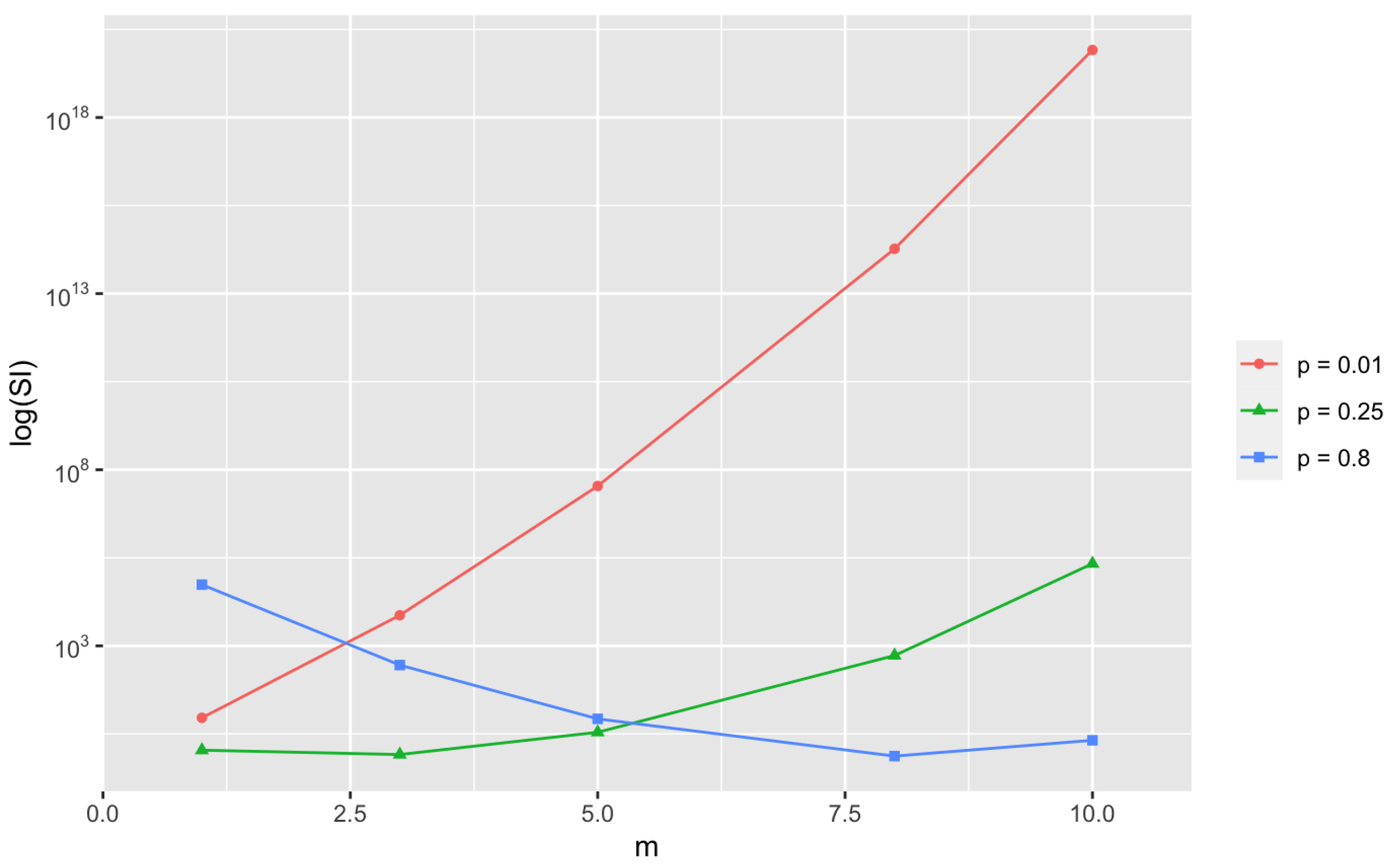
    • For p = 0.8 as m increases, the log ( S I ) value decreases, i.e., equivalently, the SI values decrease.
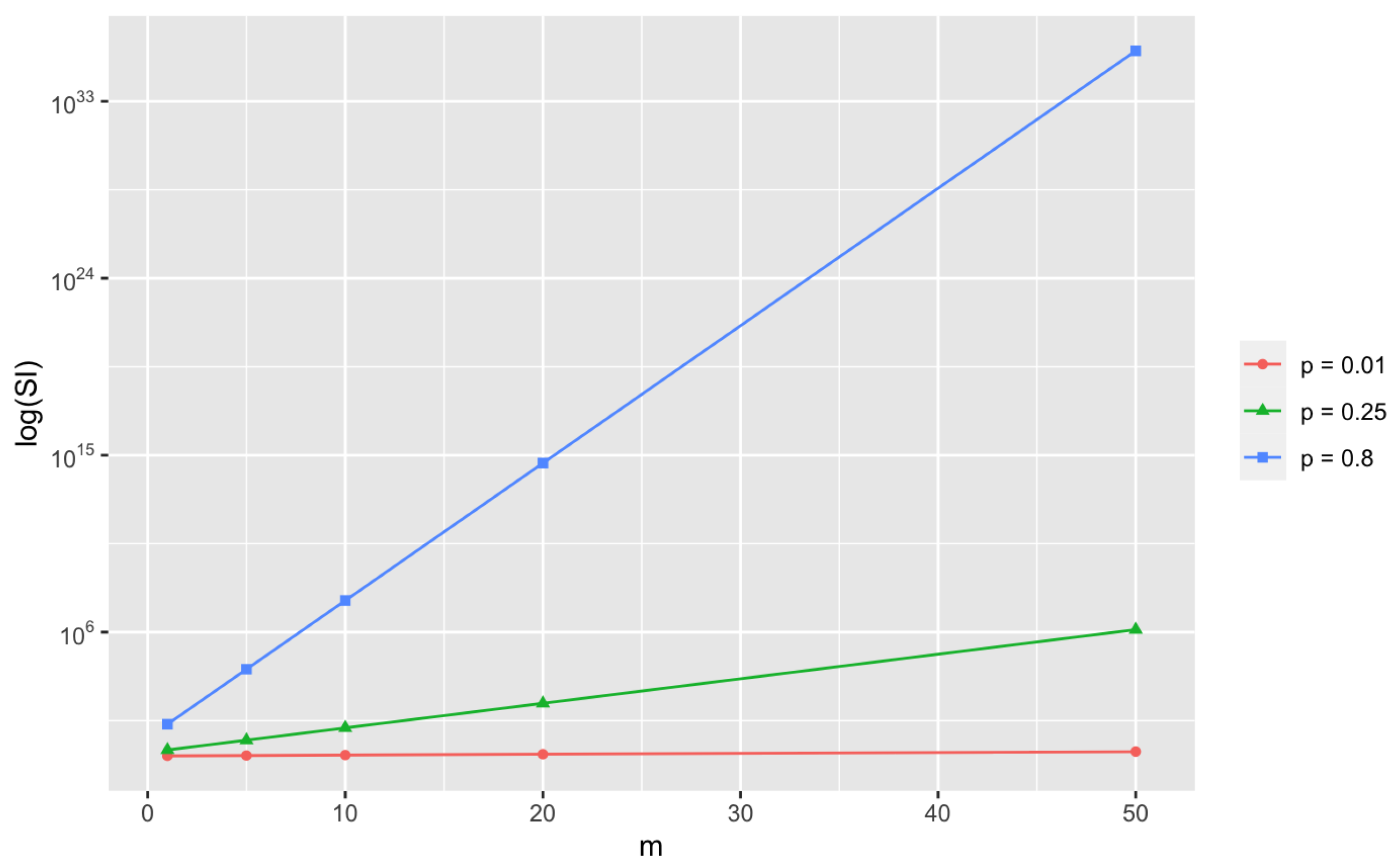
  • Observations from Figure A2: For all fixed choices of p , as m increases, the log ( S I ) value increases, i.e., equivalently, the SI values increase.
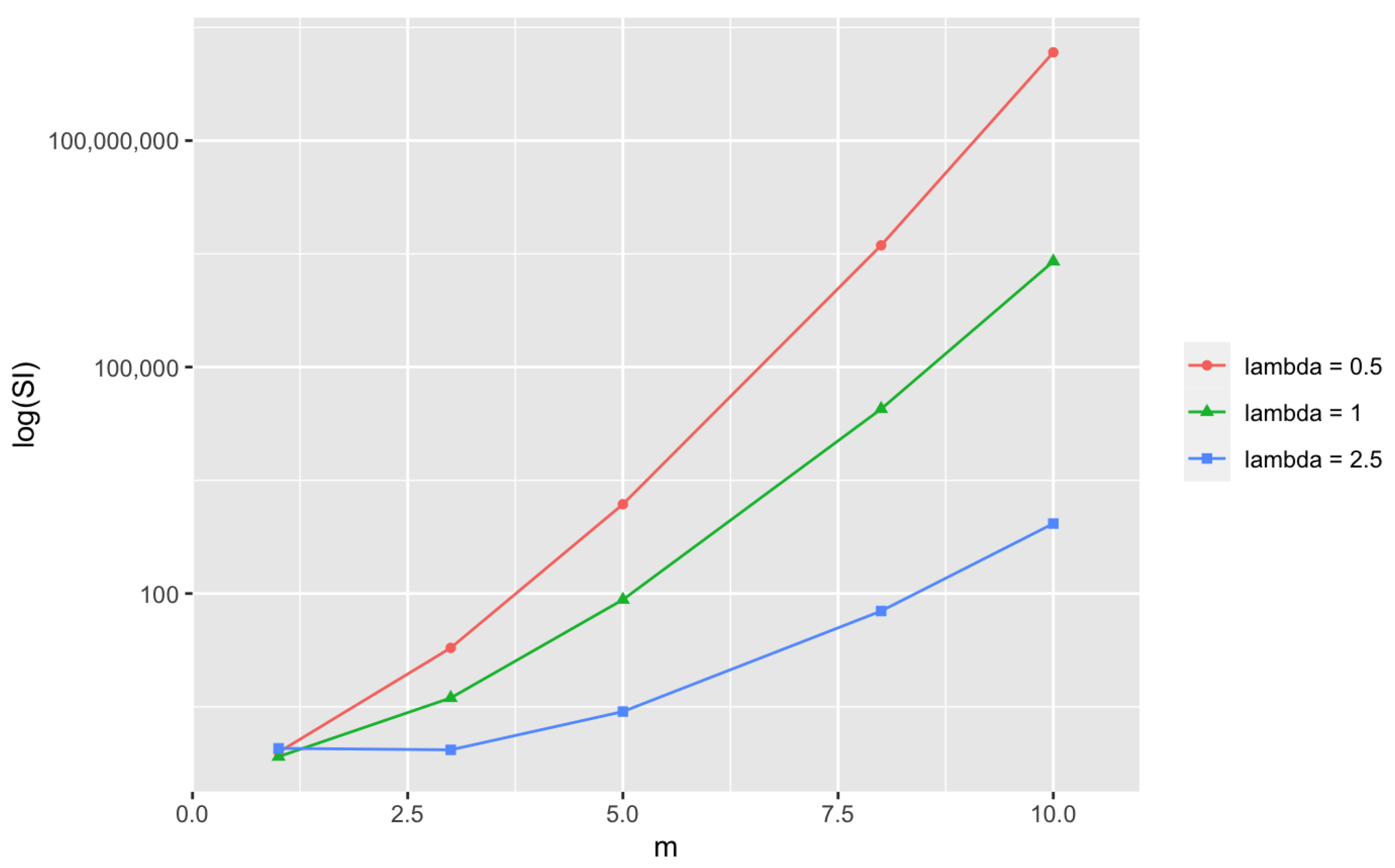
  • Observations from Figure A3: For all fixed choices of λ , as m increases, the log ( S I ) value increases, i.e., equivalently, the SI values increase; however, the magnitude of increment decreases as λ becomes larger.
  • Observations from Figure A4: The pattern is almost similar to Figure A3.
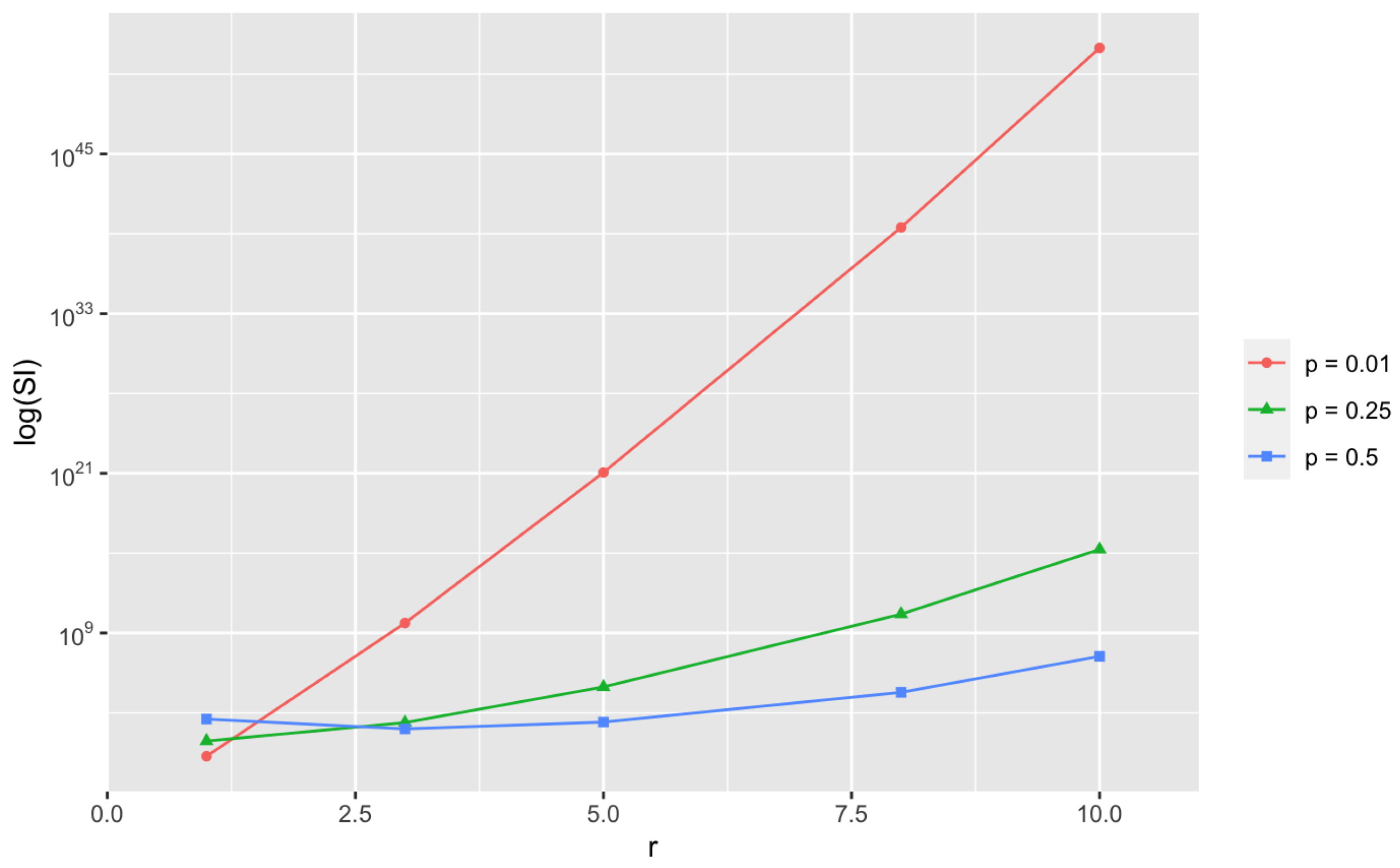
  • Observations from Figure A5:
    • When p = 0.01 , log ( S I ) takes a constant value for all choices m .
    • For p = 0.25 , 0.8 , as m increases, the log ( S I ) value increases, i.e., equivalently, the SI values increase.
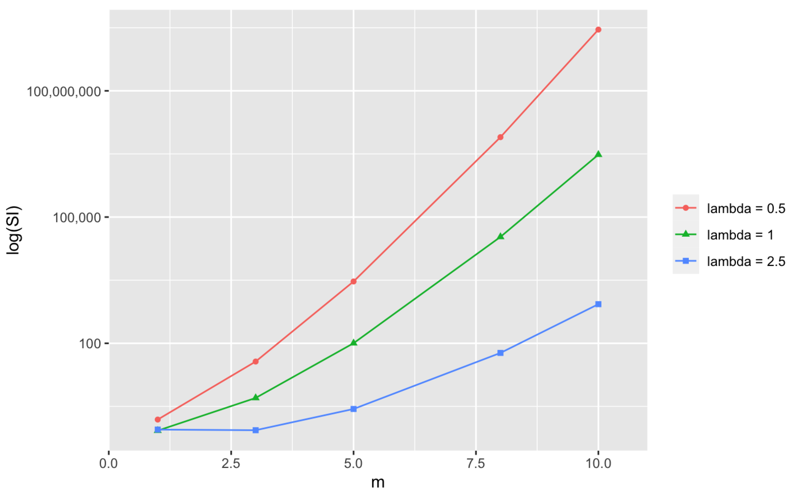
Figure A1. Surprise index values for binomial distribution, n = 10.
Mathematics 11 03234 g0a1
Figure A2. Surprise index values for negative binomial distribution, n = 10.
Mathematics 11 03234 g0a2
Figure A3. Surprise index values for Poisson distribution.
Mathematics 11 03234 g0a3
Figure A4. Surprise index values for zero-truncated Poisson distribution.
Mathematics 11 03234 g0a4
Figure A5. Surprise index values for geometric distribution.
Mathematics 11 03234 g0a5

References

  1. Weaver, W. Probability, rarity, interest, and surprise. Sci. Mon. 1948, 67, 390–392. [Google Scholar] [CrossRef]
  2. Good, I.J. The surprise index for the multivariate normal distribution. Ann. Math. Stat. 1956, 27, 1130–1135. [Google Scholar] [CrossRef]
  3. Redheffer, R.M. A note on the surprise index. Ann. Math. Stat. 1951, 22, 128–130. [Google Scholar] [CrossRef]
  4. Borja, M.C. Outliers in Long-Tailed Discrete Data. 2012. Available online: https://web-archive.lshtm.ac.uk/csm.lshtm.ac.uk/wp-content/uploads/sites/6/2016/04/Mario-Cortina-Borja-16-11-2012.pdf (accessed on 16 June 2023).
  5. Scotti, C. Surprise and uncertainty indexes: Real-time aggregation of real-activity macro-surprises. J. Monet. Econ. 2016, 82, 1–19. [Google Scholar] [CrossRef] [Green Version]
  6. David, F.N.; Johnson, N.L. The truncated poisson. Biometrics 1952, 8, 275–285. [Google Scholar] [CrossRef]
  7. Kemp, C.D.; Kemp, A.W. Some properties of the ‘Hermite’ distribution. Biometrika 1965, 52, 381–394. [Google Scholar] [PubMed]
  8. Kumar, S.C.; Ramachandran, R. On some aspects of a zero-inflated overdispersed model and its applications. J. Appl. Stat. 2020, 47, 506–523. [Google Scholar] [CrossRef] [PubMed]
  9. Moriña, D.; Higueras, M.; Puig, P.; Oliveira Pérez, M. Generalized Hermite Distribution Modelling with the R Package Hermite. 2015. Available online: https://journal.r-project.org/archive/2015/RJ-2015-035/index.html (accessed on 22 June 2023).
  10. Sellers, K.F. A distribution describing differences in count data containing common dispersion levels. Adv. Appl. Stat. Sci. 2012, 7, 35–46. [Google Scholar]
  11. Vernic, R. A multivariate generalization of the generalized Poisson distribution. ASTIN Bull. J. IAA 2000, 30, 57–67. [Google Scholar] [CrossRef]
Table 1. Surprise index values for binomial distribution for various choices of m, p, and q.
nmpq p i S i
1010.010.990.09149.04
1030.010.990.00017387.44
1050.010.99 0.00803 34,478,242.41
1080.010.99 4.41 × 10 15 1.87 × 10 14
10100.010.99 1.00 × 10 20 8.26 × 10 19
1010.250.750.18771.09
1030.250.750.25030.82
1050.250.750.05843.52
1080.250.750.0004531.61
10100.250.750.000001215,301.13
1010.80.20.00000454,639.75
1030.80.20.0008284.58
1050.80.20.02648.47
1080.80.20.301990.74
10100.80.20.10742.08
Table 2. Surprise index values for negative binomial distribution for various choices of r, m, and p.
nmpq p i S i
190.010.990.00910.55
370.010.990.000035,616,123,374.28
550.010.990.00000001 1.15 × 10 21
820.010.99 3.53 × 10 15 2.98 × 10 39
1000.010.99 1.00 × 10 20 9.32 × 10 52
190.250.750.01887.61
370.250.750.0751185.21
550.250.750.029288,714.07
820.250.750.0003 2.63 × 10 10
1000.250.750.000001 1.93 × 10 15
190.50.50.0010341.33
370.50.50.035261.81
550.50.50.1230203.05
820.50.50.035234,684.81
1000.50.50.001017,668,300.52
Table 3. Surprise index values for Poisson distribution for various choices of λ .
λ m p i S i
0.510.30331.54
0.530.012636.86
0.550.00022948.77
0.580.000000067,926,282.59
0.510 1.63 × 10 10 2,853,461,732.66
110.36790.84
130.06135.03
150.0031100.63
189,123,994.0833,812.86
1100.00000013,043,157.28
2.510.20520.89
2.530.21380.86
2.550.06682.75
2.580.003159.08
2.5100.0002850.81
Table 4. Surprise index values for zero-truncated Poisson distribution for various choices of λ .
λ m p i S i
0.510.77070.79
0.530.032119.05
0.550.00041523.94
0.580.00000014,096,347.51
0.510 4.14838 × 10 10 1,474,685,102.05
110.58200.69
130.09704.14
150.004882.89
180.0000127,850.21
1100.00000022,506,518.52
2.510.22360.89
2.530.23290.85
2.550.07282.73
2.580.003458.65
2.5100.0002844.61
Table 5. Surprise index values for the Geometric distribution for various choices of p.
mpq p i S i
10.010.990.010.51
50.010.990.00960.53
100.010.990.009140.56
200.010.990.00830.62
500.010.990.00610.84
10.250.750.251.02
50.250.750.07913.21
100.250.750.018813.53
200.250.750.0011240.26
500.250.750.00000021,345,356.92
10.80.20.820.83
50.80.20.001313,020.83
100.80.20.000000440,690,104.16
200.80.2 4.19 × 10 14 3.97 × 10 14
500.80.2 4.50 × 10 35 3.70 × 10 35
Table 6. Surprise index expressions for several continuous probability models.
DistributionSurprise Index
Uniform ( a , b ) 1 b a 1 × exp b b a a 1 / ( b a ) × e 1
Beta( a , b ) exp ( Γ [ a ] Γ [ b ] ( P o l y G a m m a [ 0 , a ] P o l y G a m m a [ 0 , a + b ] ) ) / Γ [ a + b ] × x a 1 1 x b 1 B a , b 1
Beta (type-II)( α , β ) exp Γ ( α + 1 ) Γ ( β 1 ) H α H β 2 Γ ( α + β ) B ( α , β ) × ( B α , β 1 + x α + β x α )
Pareto (type-II) exp ψ ( 0 ) ( α ) log ( σ ) + γ × α σ 1 + x σ α + 1 1
Gamma α , β exp 1 β α Γ ( α ) × β α Γ ( α ) log 1 β ψ ( 0 ) ( α ) × 1 β α Γ ( α ) x α 1 exp ( x β ) 1
Weibull k , λ exp log 1 λ k + γ k × k λ x λ k 1 exp ( ( x λ ) k ) 1
Log-normal μ , σ exp μ × 1 x 2 π σ exp log x μ 2 2 σ 2 1
Exponentiated-exponential α , β exp j = 0 α 1 j ( 1 ) j α λ ( log ( ( j + 1 ) λ ) + γ ) j λ + λ × α λ 1 exp ( λ x α 1 exp ( λ x ) 1
Note: For a Pareto (type-IV) distribution, the associated integral for the numerator of Equation (19) diverges.
Disclaimer/Publisher’s Note: The statements, opinions and data contained in all publications are solely those of the individual author(s) and contributor(s) and not of MDPI and/or the editor(s). MDPI and/or the editor(s) disclaim responsibility for any injury to people or property resulting from any ideas, methods, instructions or products referred to in the content.