Enhancing Decomposition Approach for Solving Multi-Objective Dynamic Non-Linear Programming Problems Involving Fuzziness

Abstract

In real-life scenarios, there are many mathematical tools to handle incomplete and imprecise data. One of them is the fuzzy approach. The main issue with addressing nonlinear interval programming (NIP) problems is that the optimal solution to the problem is a decision made under uncertainty that has a risk of not satisfying the feasibility and optimality criteria. Some strategies handle this kind of problem using classical terminology such as optimal solution and feasible solution. These strategies are insufficient for efficient analysis since the properties of the solution in an uncertain environment are ignored. Therefore, in the proposed approach, more suitable terminologies were suggested for the analysis process. In addition, it combines parametric treatment and interactive methodology. This article aims to contribute to the literature of fuzzy multi-objective dynamic programming (MODP) issues involving the fuzzy objective functions. The piecewise quadratic fuzzy numbers characterize these fuzzy parameters. Some basic notions in the problem under the α-pareto optimal solution concept is redefined and analyzed to study the stability of the problem. Furthermore, a technique, named the decomposition approach (DP), is presented for achieving a subset for the parametric space that contains the same α-pareto optimal solution. For a better understanding of the suggested concept, a numerical example is provided.

1. Introduction

One of the most essential methodologies for solving optimization problems is dynamic programming (DP), where the so-called principle of optimality, as defined by Bellman [1] is used to create its methods. The multi-objective dynamic programming (MODP) is a method for resolving problems with competing objective functions that follows the DP properties (Mine and Fukushima [2]; Carraway et al. [3]; Abo-Sinna and Hussein [4]; Abo-Sinna and Hussein [5]).

Osman [6,7] introduced the ideas of solvability set, the stability sets of the first kind and second kind, as well as the analysis of these terms for parametric convex non-linear programming problem. For certain classes of multi-objective convex programming problems Osman and Dauer [8] provided a technique to compute this set and the related pareto optimum solution.

First, Zadeh [9] presented the philosophy of fuzziness in the literature, which can be applied to deal with the issues in real-life scenario where the information is in the form of ambiguousness and incompleteness. Bellman and Zadeh [10] created a method for solving decision-making problems involving fuzziness that improved and aided managerial decision making. Linear programming, along with fuzzy programming involving numerous objective functions, was presented by Zimmermann [11]. Several people afterwards worked in the field of fuzziness. As a result of the convenience, the piecewise linear fuzzy numbers such as interval, triangular, trapezoidal, pentagonal, hexagonal fuzzy numbers, etc. have been applied in the literature [12,13,14,15,16]. Many authors have investigated the solution methodology as well as their applications involving fuzziness, fuzzy systems, and fuzzy mathematical programming problems [17,18]. There are several papers dealing with uncertainty (for example, Fei et al. [19]; and Nguyen et al. [20]).

In the literature, fuzzy dynamic programming models in particular have received a lot of attention (see, Zimmermann [21]; Esogbue [22]; Esogbue and Bellman [23]; Hussein and Abo-Sinna [24]). Tanaka and Asai [25] introduced fuzzy parameters to multi-objective linear programming (MOLP) problems. General fuzzy multi-objective non-linear programming (MONLP) models were formulated by Orlovski [26]. Sakawa and Yano [27,28] developed the idea of pareto optimum optimality and proposed a new interactive fuzzy approach for MOLP and MONLP issues with fuzzy parameters. For fuzzy MONLP situations, Osman and El-Banna [29] proposed a qualitative analysis and stability. There are many researchers who have developed MODP (for instance, Moghaddam and Ghoseiri [30]; Muruganantham et al. [31]; Li et al. [32]; Deng et al. [33]; Besheli et al. [34]; Peraza et al. [35]; Azevedo et al. [36]; Ni et al. [37]; Wu et al. [38]; Liu et al. [39]; Zou et al. [40]; and Zhang et al. [41]).

Based on a survey of the literature, in this article, the parameters of the model are re-defined and further studied for MODP problems involving the fuzzy parameters in objective functions.

The main contributions of this article are as follows:

(i)

For the core terminology associated with the problem of stability in non-linear programming, the parameters are rearranged to study the case of MODP.

(ii)

An algorithm for computing the subset of the parametric space that possesses the same associated pareto optimal solution, is developed.

(iii)

The first-kind stability set is defined and determined.

The following is how the paper is structured: Section 2 gives the preliminaries and some background information on piecewise quadratic fuzzy numbers and their $\alpha$-levels and the arithmetic operations. Section 3 formulates multi-objective dynamic programming in fuzzy environments. The stability sets of the first kind are defined and determined in Section 4. Section 5 proposes a decomposition algorithm for determining the $\alpha$-pareto optimal solution. Section 6 presents a numerical example to demonstrate the DP algorithm. Section 7 develops a comparison of the proposed study with the existing relevant literature, the advantages, and the limitations of the proposed algorithm. Finally, some concluding remarks and future works are reported in Section 8.

2. Preliminaries

In this section, we recall some basic concepts that will help the readers to understand the proposed work.

Definition 1. 

(Jain [42]). A piecewise quadratic fuzzy number (PQFN) is designated by ${\tilde{A}}_{PQ}=\left(b_1,b_2,b_3,b_4,b_5\right)$, where $b_1\le b_2\le b_3\le b_4\le b_5$ are real numbers, and its membership function ${\mu }_{{\tilde{A}}_{PQ}}$ is given by the following expression (please see  Figure 1 ).

$${\mu }_{{\tilde{A}}_{PQ}}=\left\{\begin{array}{c}0,\hspace{1em}\hspace{1em}\hspace{1em}\hspace{1em}\hspace{1em}x<b_1;\\ \frac{1}{2}\frac{1}{{\left(b_2-b_1\right)}^2}{\left(x-b_1\right)}^2,\hspace{1em}{b}_1\le x\le b_2;\\ \frac{1}{2}\frac{1}{{\left(b_3-b_2\right)}^2}{\left(x-b_3\right)}^2+1,\hspace{1em}\hspace{1em}{b}_2\le x\le b_3;\\ \frac{1}{2}\frac{1}{{\left(b_4-b_3\right)}^2}{\left(x-b_3\right)}^2+1,\hspace{1em}{b}_3\le x\le b_4;\\ \frac{1}{2}\frac{1}{{\left(b_5-b_4\right)}^2}{\left(x-b_5\right)}^2,\hspace{1em}{b}_4\le x\le b_5;\\ 0,\hspace{1em}\hspace{1em}\hspace{1em}\hspace{1em}\hspace{1em}x>b_5.\end{array}\right.$$

Figure 1. Graph Illustration of a PQFN.

Definition 2. 

(Jain [42]). For a given PQFN $\tilde{A}$, the interval approximation, denoted by $\left[{\tilde{A}}_{PQ}\right]=\left[p_{\alpha }^L,p_{\alpha }^U\right]$, is called the closed interval approximation, when the below-mentioned condition is satisfied:

$$p_{\alpha }^L=\mathit{inf}\left\{y\in \mathfrak{R}:{\mu }_{{\tilde{A}}_{PQ}}\ge 0.5\right\}, and p_{\alpha }^U=\mathit{sup}\left\{y\in \mathfrak{R}:{\mu }_{{\tilde{A}}_{PQ}}\ge 0.5\right\}.$$

Definition 3. 

(Jain [42]). Suppose that ${\tilde{a}}_{PQ}=\left(p_1,p_2,p_3,p_4,p_5\right)$ and  ${\tilde{b}}_{PQ}=\left(q_1,q_2,q_3,q_4,q_5\right)$ be two PQFNs. Then

(i)

Addition:  ${\tilde{a}}_{PQ}\oplus {\tilde{b}}_{PQ}=\left(p_1+q_1,p_2+q_2,p_3+q_3,p_4+q_4,p_5+q_5\right)$.

(ii)

Subtraction:  ${\tilde{a}}_{PQ}\ominus {\tilde{b}}_{PQ}=\left(p_1-q_5,p_2-q_4,p_3-q_3,p_4-q_2,p_5-q_1\right).$

(iii)

Scalar multiplication:  $\alpha .{\tilde{b}}_{PQ}=\left\{\begin{array}{c}\left(\alpha q_1,\alpha q_2,{\alpha q}_3,{\alpha q}_4,\alpha q_5\right),\alpha >0,\\ \left(\alpha q_5,\alpha q_4,{\alpha q}_3,{\alpha q}_2,\alpha q_1\right),\alpha <0.\end{array}\right.$

Definition 4. 

(Jain [42]). Suppose $\left[\mathrm{A}\right]=\left[p_{\alpha }^L,p_{\alpha }^U\right]$, and $\left[\mathrm{B}\right]=\left[q_{\alpha }^L,q_{\alpha }^U\right]$ are two inexact intervals for the PQFN. Then, the arithmetic rules are presented as follows:

(i)

$\left[\mathrm{A}\right]\oplus \left[\mathrm{B}\right]=\left[p_{\alpha }^L+q_{\alpha }^L,p_{\alpha }^U+q_{\alpha }^U\right],$

(ii)

$\left[\mathrm{A}\right]\ominus \left[\mathrm{B}\right]=\left[p_{\alpha }^L-q_{\alpha }^U,p_{\alpha }^U-q_{\alpha }^L\right],$

(iii)

$\alpha \left[\mathrm{A}\right]=\left\{\begin{array}{c}\left[\alpha p_{\alpha }^L,{\alpha p}_{\alpha }^U\right],\alpha >0,\\ \left[\alpha p_{\alpha }^U,\alpha p_{\alpha }^L\right],\alpha <0.\end{array}\right.$

(iv)

$\left[\mathrm{A}\right]\odot \left[\mathrm{B}\right]=\left[\frac{p_{\alpha }^U{q}_{\alpha }^L+p_{\alpha }^L{q}_{\alpha }^U}{2},\frac{p_{\alpha }^L{q}_{\alpha }^L+p_{\alpha }^U{q}_{\alpha }^U}{2}\right].$

(v)

$\frac{\left[\mathrm{A}\right]}{\left[\mathrm{B}\right]}=\left\{\begin{array}{c}\left[\frac{2p_{\alpha }^L}{q_{\alpha }^L+q_{\alpha }^U},\frac{2p_{\alpha }^U}{q_{\alpha }^L+q_{\alpha }^U}\right],\left[\mathrm{B}\right]>0 \mathit{and} q_{\alpha }^L+q_{\alpha }^U\ne 0,\\ \left[\frac{2q_{\alpha }^U}{q_{\alpha }^L+q_{\alpha }^U},\frac{2q_{\alpha }^L}{q_{\alpha }^L+q_{\alpha }^U}\right],\left[\mathrm{B}\right]<0 \mathit{and} q_{\alpha }^L+q_{\alpha }^U\ne 0.\end{array}\right.$

Definition 5. 

(Jain [42]). The order relations, authenticated by the symbols $\left\{{{=}_{LU},\le }_{LU}{,\ge }_{LU}\right\},$ for the intervals $\left[\mathrm{A}\right]$ and $\left[\mathrm{B}\right]$ are designated as follows:

(i)

$\left[\mathrm{A}\right]{=}_{(L,U)}\left[\mathrm{B}\right]$ if $p_{\alpha }^L=q_{\alpha }^L$ and $p_{\alpha }^U=q_{\alpha }^U.$

(ii)

$\left[\mathrm{A}\right]\left({\le }_{(L,U}\right)\left[\mathrm{B}\right]$ if $p_{\alpha }^L\left({\le }_{(L,U)}\right)q_{\alpha }^L$ and $p_{\alpha }^U\left({\le }_{(L,U}\right)q_{\alpha }^U$ or  $p_{\alpha }^L+p_{\alpha }^U\left({\le }_{(L,U)}\right)q_{\alpha }^L+q_{\alpha }^U.$

(iii)

$\left[\mathrm{A}\right]\left({\ge }_{(L,U}\right)\left[\mathrm{B}\right]$ if $p_{\alpha }^L\left({\ge }_{(L,U)}\right)q_{\alpha }^U$ and $p_{\alpha }^U\left({\ge }_{(L,U}\right)q_{\alpha }^L$ or $p_{\alpha }^L+p_{\alpha }^U\left({\ge }_{(L,U}\right)q_{\alpha }^U+q_{\alpha }^L.$

3. Problem Statement and Solution Concepts

In general, the fuzzy multi-objective dynamic programming (PQF-MODP) problem is considered. In this paper is the following piecewise quadratic fuzzy vector-minimization problem (PQF-VMP) involving fuzzy parameters in the objective functions.

$$\min G_l\left(g_{l1}\left(x_1,{\tilde{a}}_1^{PQ}\right),g_{l2}\left(x_2,{\tilde{a}}_2^{PQ}\right),\dots ,g_{lN}\left(x_N,{\tilde{a}}_N^{PQ}\right)\right),l=1,\dots ,L;,L\ge 2$$

(1)

Subject to (1)

$$H_q\left(h_{q1}\left(x_1\right),h_{q2}\left(x_2\right),\dots ,h_{QN}\left(x_N\right)\right)\le 0,q=1,2,\dots ,Q$$

$$x_n\in X_n,n=1,\dots ,N$$

where $X_n\subset {\mathfrak{R}}^{r_n},n=1,\dots ,N;x_n$ is an $r_n$ vector, the objective functions denoted by $G_l,l=1,\dots ,L$ and the constraint functions $H_q,q=1,\dots ,Q$ are convex real-valued functions of class ${\complement }^{\left(1\right)}$ on ${\mathfrak{R}}^N$ and $g_{ln},h_{qn}.l=1,\dots ,L;q=1,\dots ,Q;n=1,\dots ,N$ are real-valued functions on $X_n$, and ${\tilde{a}}^{PQ}=\left({\tilde{a}}_{11}^{PQ},{\tilde{a}}_{22}^{PQ},\dots ,{\tilde{a}}_{ln}^{PQ}\right),l=1,\dots ,L;n=1,\dots ,N$ represents a vector of fuzzy parameters in the objective functions $f_{ln}\left(x_n,{\tilde{a}}_{ln}^{PQ}\right).$ In the problem statement and solution concept, it is assumed that the fuzzy parameters are designated as per the work of Jain [42], and the PQF-VMP is stable (Rockafellar [43]).

Definition 6. 

([17]). The $\alpha$-level set of the fuzzy numbers ${\tilde{a}}_{ln}^{PQ}$ refers to the ordinary set  $L_{\alpha }\left({\tilde{a}}_{ln}^{PQ}\right)$ for which the degree of their membership functions exceed the level $\alpha \in \left[\mathrm{0,1}\right]$ as described below in Equation (2):

$$L_{\alpha }\left({\tilde{a}}_{ln}^{PQ}\right)=\left(a:{\mu }_{{\tilde{a}}_{ln}^{PQ}}\left(a_{ln}\right)\ge \alpha ,l=1,2,\dots ,L;n=1,\dots ,N\right)$$

(2)

For a certain degree of $\alpha ,$ the (PQF-VMP) problem is converted into the problem (Sakawa and Yano [27]) and is illustrated as in following problem (3):

$$(\alpha \text{-}\mathit{VMP})\mathit{min}{G}_l\left(g_{l1}\left(x_1,a_1\right),g_{l2}\left(x_2,a_2\right),\dots ,g_{lN}\left(x_N,a_N\right)\right),l=1,\dots ,L;L\ge 2$$

(3)

Subject to (3)

$$H_q\left(h_{q1}\left(x_1\right),h_{q2}\left(x_2\right),\dots ,h_{QN}\left(x_N\right)\right)\le 0,q=1,\dots ,Q;{a_{ln}\in L}_{\alpha }\left({\tilde{a}}_{ln}^{PQ}\right),$$

$$x_n\in X_n,n=1,\dots ,N.$$

Since the (PQF-VMP) problem becomes stable, it therefore implies that the ($\alpha$-VMP) is also stable.

Definition 7. 

(Mine and Fukushima [2]). (Separability and Monotonicity) The objective function $G_l$ is called separable if there exist functions  $G_l^n,n=1,\dots N,$ defined on  ${\mathfrak{R}}^n$ and functions  ${\Omega }_l^n$ designated on  ${ \mathfrak{R}}^2$ satisfying for  $n=2,\dots ,N$,

$$\begin{gathered} G_l^n\left(g_{l1}\left(x_1,a_1\right),g_{l2}\left(x_2,a_2\right),\dots ,g_{ln}\left(x_n,a_n\right)\right) \\ ={\Omega }_l^n\left(G_l^{n-1}\left(g_{l1}\left(x_1,a_1\right),g_{l2}\left(x_2,a_2\right),\dots ,g_{ln-1}\left(x_{n-1},a_{n-1}\right)\right),g_{ln}\left(x_n,a_n\right)\right) \end{gathered}$$

 and

$$G_l^N\left(g_{l1}\left(x_1,a_1\right),g_{l2}\left(x_2,a_2\right),\dots ,g_{lN}\left(x_N,a_N\right)\right)=G_l\left(g_{l1}\left(x_1,a_1\right),g_{l2}\left(x_2,a_2\right),\dots ,g_{lN}\left(x_N,a_N\right)\right)$$

Similarly, the constraint function  $H_q$ is separable, if there exist some functions  $H_q^n,n=1,\dots ,N,$ defined on  ${\mathfrak{R}}^n$  and  ${\chi }_q^n,n=1,\dots ,N,$  on  ${\mathfrak{R}}^2$ satisfying for  $n=2,\dots ,N,$

$$\begin{gathered} H_q^n\left(h_{q1}\left(x_1\right),h_{q2}\left(x_2\right),\dots ,h_{Qn}\left(x_n\right)\right) \\ ={\chi }_q^n\left(H_q^{n-1}\left(h_{q1}\left(x_2\right),h_{q2}\left(x_2\right),\dots ,h_{qn-1}\left(x_{n-1}\right),h_{Qn}\left(x_n\right)\right)\right) \end{gathered}$$

 and

$$H_q^n\left(h_{q1}\left(x_1\right),h_{q2}\left(x_2\right),\dots ,h_{QN}\left(x_N\right)\right)=H_q\left(h_{q1}\left(x_1\right),h_{q2}\left(x_2\right),\dots ,h_{QN}\left(x_N\right)\right),$$

If all objective functions as well as constraints are separable, we can imply that $(\alpha$-VMP) is separable. Moreover, the functions ${\Omega }_l^n$ and ${\chi }_q^n$ are called the separating functions of $G$ and $H.$

Furthermore, the separation of $(\alpha$-VMP) is said to be monotone if all functions ${\Omega }_l^n$ and ${\chi }_q^n$ are strictly increasing with respect to the first argument for each fixed second argument. Specifically, for each $y\in \mathfrak{R}$, ${\Omega }_l^n\left(r,y\right)>{\Omega }_l^n\left(\widehat{r},y\right)iffr>\widehat{r},$ and ${\chi }_l^n\left(r,y\right)>{\chi }_l^n\left(\widehat{r},y\right)⟺r>\widehat{r}$, for every $L=1,\dots ,L;q=1,\dots ,Q;$ and $n=1,\dots ,N.$

Based on Definition 6, the concept of the $\alpha$-pareto optimal solution to the $(\alpha$-VMP) is introduced as follows:

Definition 8. 

($\alpha$-pareto optimal solution). The feasible solution  $x^{*}=\left(x_1^{*},x_2^{*},\dots ,x_N^{*}\right),a^{*}=\left(a_1^{*},a_2^{*},\dots ,a_N^{*}\right)$ to the ($\alpha$-VMP) is referred to as an  $\alpha$-pareto optimal solution provided that we do not find the feasible  $\left(x_1^{\prime },x_2^{\prime },\dots ,x_N^{\prime }\right),a^{*}=\left(a_1^{\prime },a_2^{\prime },\dots ,a_N^{\prime }\right)\in L_{\alpha }\left({\tilde{a}}_{ln}^{PQ}\right)$ such that

$$G_l\left(g_{l1}\left(x_1^{\prime },a_1^{\prime }\right),g_{l2}\left(x_2^{\prime },a_2^{\prime }\right),\dots ,g_{ln}\left(x_N^{\prime },a_N^{\prime }\right)\right)\le G_l\left(g_{l1}\left(x_1^{*},a_1^{*}\right),g_{l2}\left(x_2^{*},a_2^{*}\right),\dots ,g_{ln}\left(x_N^{*},a_N^{*}\right)\right)$$

 for all  $l$, and

$$G_r\left(g_{s1}\left(x_1^{\prime },a_1^{\prime }\right),g_{s2}\left(x_2^{\prime },a_2^{\prime }\right),\dots ,g_{sn}\left(x_N^{\prime },a_N^{\prime }\right)\right)<G_r\left(g_{s1}\left(x_1^{*},a_1^{*}\right),g_{s2}\left(x_2^{*},a_2^{*}\right),\dots ,g_{sn}\left(x_N^{*},a_N^{*}\right)\right),$$

 for at least one index  $s\in \left\{1,2,\dots ,L\right\},$ where the corresponding values of parameters  $a^{*}$are called  $\alpha$-level optimal parameters.

Assumption 1. 

The ($\alpha$-VMP) is separable and the separable is monotone.

Assumption 2. 

For every  $n, the set X_n\cap L_{\alpha }\left(\tilde{a}\right)$ is assumed to be compact and

$$G_l^n\left(g_{l1}\left(x_1,a_1\right),g_{l2}\left(x_2,a_2\right),\dots ,g_{ln}\left(x_n,a_n\right)\right),l=1,\dots ,L,$$

 and

$$H_q^n\left(h_{q1}\left(x_1\right),h_{q2}\left(x_2\right),\dots ,h_{Qn}\left(x_n\right)\right),q=1,\dots Q;n=1,\dots N,$$

 are continuous functions of $\left(x_1,x_2,\dots ,x_n\right)$ and $\left(a_1,a_2,\dots ,a_n\right)$.

Based on the weighting method (as presented by Chankong and Haimes [44]), $(\alpha$-VMP) can be treated as follows:

$$\left(\alpha \text{-}{VPM}_w\right)\hspace{1em}\mathit{min}{\sum }_{l=1}^L{w}_l{G}_l\left(g_{l1}\left(x_1,a_1\right),g_{l2}\left(x_2,a_2\right),\dots ,g_{lN}\left(x_N,a_N\right)\right),$$

(4)

Subject to (4)

$$H_q\left(h_{q1}\left(x_1\right),h_{q2}\left(x_2\right),\dots ,h_{QN}\left(x_N\right)\right)\le 0,q=1,\dots Q;{a\in L}_{\alpha }\left(\tilde{a}\right),$$

$$x_n\in X_n,n=1,\dots ,N;w\in W=\left\{w\in {\mathfrak{R}}^L:{\sum }_{l=1}^L{w}_l=1,w_l\ge 0\right\}.$$

It is easy to see that the stability of the  $(\alpha$-VMP) problem implies to the stability of ($\alpha$-VMP_w). In addition, it is well known that  $\left(x^{*},a^{*}\right)$ is an  $\alpha$-pareto optimal solution of  $(\alpha$-VMP) if there exists  $w^{*}\ge 0, w^{*}\ne 0$ such that  $x^{*}$is the unique optimal solution if and only if there exists  $w^{*}=\left(w_1^{*},\dots ,w_L^{*}\right)>0,$ provided every  $X_n\cap L_{\alpha }\left({\tilde{a}}_{ln}^{PQ}\right)$ is closed and convex.

Suppose that every  $G_l$ follows the addition rule, i.e., for  $l=1,\dots ,L,$ we have

$$G_l\left(g_{l1}\left(x_1,a_1\right),g_{l2}\left(x_2,a_2\right),\dots ,g_{lN}\left(x_N,a_{nN}\right)\right)={\overline{g}}_{l1}\left(x_1,a_1\right),{\overline{g}}_{l2}\left(x_2,a_2\right),\dots ,{\overline{g}}_{LN}\left(x_N,a_{nN}\right)$$

Thereafter, the objective function in  $(\alpha$-VMP_w) becomes

$${\sum }_{n=1}^N{\sum }_{l=1}^L{w}_l{\overline{g}}_{Ln}\left(x_n,a_n\right)={\sum }_{n=1}^{N}w{g}_n\left(x_n,a_n\right)$$

If we define the real valued function  $A_n\left(w,u\right)$ for each  $n=1,\dots ,N,$ each  $w=\left(w_1,\dots ,w_L\right)>0,$ and  $u=\left(u_1,\dots ,u_Q\right)$ as illustrated in the following Equation (5)

$$A_n\left(w,u\right)=min\left\{\begin{array}{c}{\sum }_{i=1}^{n}w{g}_i\left(x_i,a_i\right):G_l^l\left(g_{l1}\left(x_1\right),g_{l2}\left(x_2\right),\dots ,g_{ln}\left(x_n\right)\right){\le u}_q,\\ q=1,\dots ,Q;x_1\in X_1,\dots ,x_n\in X_n,n=1,\dots ,N;{a\in L}_{\alpha }\left({\tilde{a}}_{ln}^{PQ}\right)\end{array}\right\}$$

(5)

The recursive relation, for  $n=1,\dots ,N,$ is presented as follows in the recursive Equation (6):

$$A_n\left(w,u\right)=\underset{{\mathit{x}}_n\in X_n,{a\in L}_{\alpha }\left({\tilde{a}}_{\mathit{ln}}^{\mathit{PQ}}\right)}{\mathit{min}}\left(A_{n-1}\left(w,u^{n-1}\left(x_n,u\right)\right)+w{g}_n\left(x_n,a_n\right)\right)$$

(6)

Here, in recursive relation (6),

$$u^{n-1}\left(x_n,u\right)=\left(u_1^{n-1}\left(x_n,u\right),\dots ,u_Q^{n-1}\left(x_n,u\right)\right).$$

Assuming the monotonicity of${ G}_l^l$, let  $u_Q^{n-1}$ be defined as follows:

$$u_Q^{n-1}\left(x_n,u\right)=\mathit{sup}\left\{\nu \in \mathfrak{R}:u_Q^{n-1}(\nu ,h_{qn}(x_n)\le u_q,q=\overline{1,Q}\right\}$$

Theorem 1. 

Suppose Assumption 1 and Assumption 2 hold. Let $\left(x_1^{*},x_2^{*},\dots ,x_n^{*}\right);\left(a_1^{*},a_2^{*},\dots ,a_n^{*}\right){\in L}_{\alpha }\left({\tilde{a}}_{ln}^{PQ}\right)$ is any $\alpha$-pareto optimal solution of $A_n\left(w^{*},u\right)$ for some $w^{*}\in W$. Then $\left(x_1^{*},x_2^{*},\dots ,x_{n-1}^{*}\right);\left(a_1^{*},a_2^{*},\dots ,a_{n-1}^{*}\right){\in L}_{\alpha }\left(\tilde{a}\right)$ would be an $\alpha$-pareto optimal solution for $A_{n-1}\left(w^{*},u^{n-1}(x_n,u)\right).$

Proof. 

(see Mine and Fukushima [2]).

By applying the recursive relation (6) for various values of $n$, we may find a set of $\alpha$-pareto optimal solutions of ($\alpha$-VMP) by obtaining $A_n\left(w,0\right)$. □

4. Stability Set of the First Kind

Definition 9. 

Given a particular  $w^{*}$ containing the corresponding  $\alpha$-pareto optimal solution  $\left(x^{*},a^{*}\right)$, the stability set of the first kind of $\left(\alpha -VMP\right)$ corresponding to $\left(x^{*},a^{*}\right)$ denoted by $S\left(x^{*},a^{*}\right)$ is defined as follows:

$$S\left(x^{*},a^{*}\right)=\left\{\left(w^{*},a^{*}\right)\in {\mathfrak{R}}^{6l}:is an \alpha -pareto optimal solution of\left(\alpha -VMP\right)\right\}$$

Here,

$${\mathfrak{R}}^{6l}={\mathfrak{R}}^{l+5l},w\in {\mathfrak{R}}^l,P=\left(p_1,p_2,p_3,p_4,p_5\right)\in {\mathfrak{R}}^{5l},l=1,\dots ,L, and L\ge 2.$$

Theorem 2. 

If the functions $G$ and $H$ are convex and ${\mu }_{{\tilde{a}}_{ln}^{PQ}}\left(a_{ln}\right)$ is a concave function, the set $S\left(x^{*},a^{*}\right)$ is convex and $S\left(x^{*},a^{*}\right)\cup \left\{0\right\}$ is closed. In addition,$int\left(S\left(x^{*},a^{*}\right)\cap S\left(x^{\prime },a^{\prime }\right)\right)\ne \varnothing$, then $S\left(x^{*},a^{*}\right)=S\left(x^{\prime },a^{\prime }\right)$.

Proof. 

(see Osman [7]). □

Remark 1. 

It must be noted that the properties of the stability set of the first kind still hold if the continuity and differentiability assumptions, which are imposed of$G$ and$H$, are relaxed [6].

Determination of the Stability Set of the First Kind

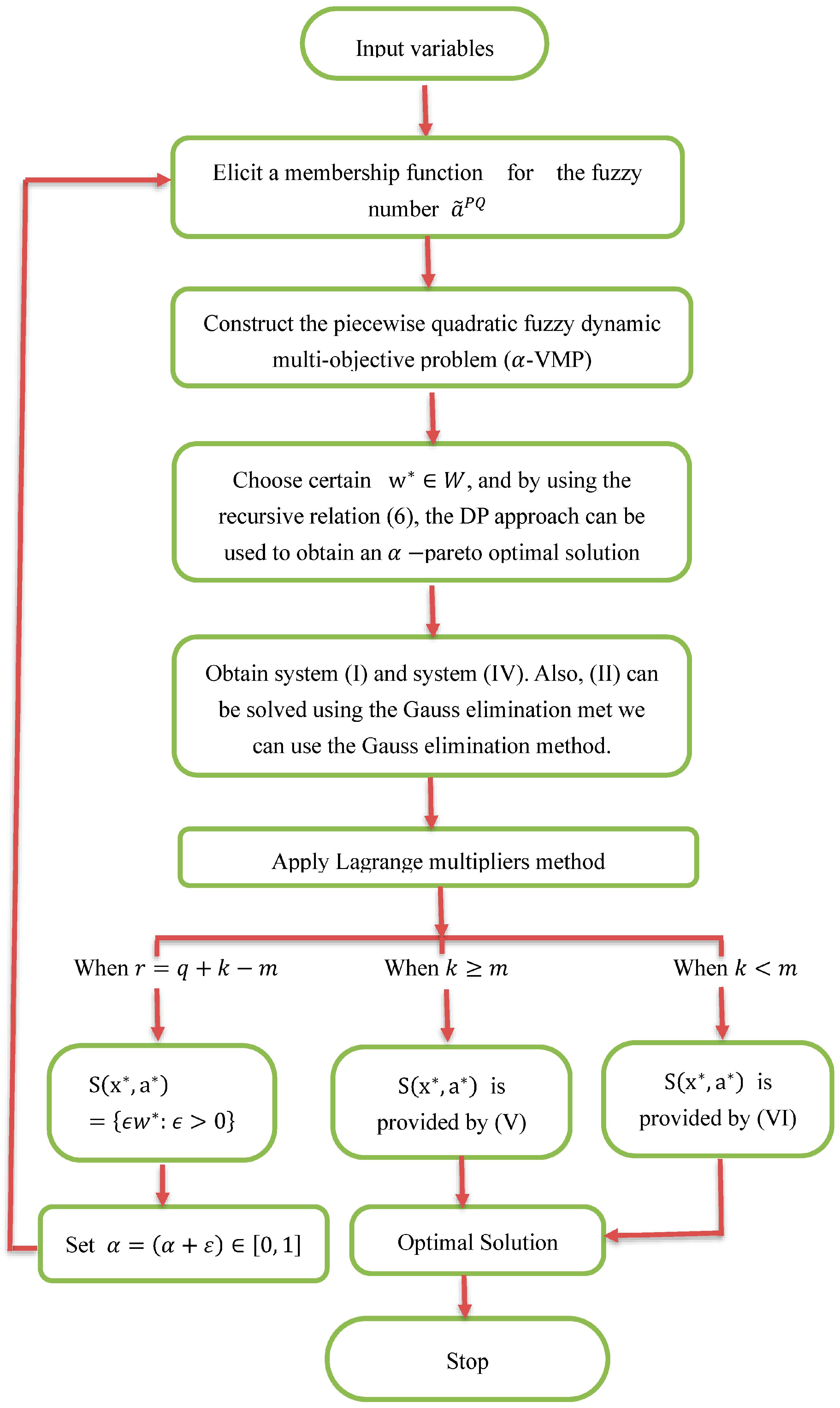
If a point $\left(x^{*},a^{*}\right)$ is an $\alpha$-pareto optimal solution for ($\alpha$-VMP), then there exists $w^{*}\in W$, such that $\left(x^{*},a^{*}\right)$ is an $\alpha$-pareto optimal solution of ($\alpha$-VMP_w). Therefore, from the stability ($\alpha$-VMP_w), it follows that there exists $w\in {\mathfrak{R}}^l,w\ge 0,E\in {\mathfrak{R}}^Q,E\ge 0$, and $F\in {\mathfrak{R}}^l,F\ge 0$, such that the following Kuhn–Tucker conditions are satisfied (Mangasarian [45]; Khalifa and Kumar [46]).

$$w^T\frac{\partial G}{\partial x}\left(x^{*},a^{*}\right)+E^T\frac{\partial H}{\partial x}\left(x^{*}\right)=0,$$

(7)

$$w^T\frac{\partial G}{\partial a}\left(x^{*},a^{*}\right)-F^T\frac{\partial {\mu }_{\tilde{a}}}{\partial a}\left(a^{*}\right)=0,$$

(8)

$${\sum }_{i=1}^n{w}_i=1,$$

(9)

$$H\left(x^{*}\right)\le 0,$$

(10)

$$\alpha -{\mu }_{\tilde{a}}\left(a^{*}\right)\le 0,$$

(11)

$$E^{T}H\left(x^{*}\right)=0,$$

(12)

$$F^T\left(\alpha -{\mu }_{\tilde{a}}\left(a^{*}\right)\right)=0,$$

(13)

$$w\ge 0,E,\mathrm{and} F\ge 0.$$

(14)

Let the two sets $B\left(x^{*}\right)$ and $I$ be defined by

$$B\left(x^{*}\right)=\left\{q:H_q\left(h_{q1}\left(x_1^{*}\right),h_{q2}\left(x_2^{*}\right),\dots ,h_{QN}\left(x_N^{*}\right)\right)=0\right\}$$

and

$$I=\left\{l\in \left\{1,2,\dots ,L\right\}:{\mu }_{{\tilde{a}}_l}\left(a_l\right)=\alpha \right\}$$

As a result, we obtain the two linear independent systems of equations as illustrated in systems (I) and (II) below.

$$w^T\frac{\partial G}{\partial x}\left(x^{*},a^{*}\right)+{\sum }_{q\in B\left(x^{*}\right)}{\gamma }_q\frac{\partial H_q}{\partial x}\left(x^{*}\right)=0,$$

(I)

$${\sum }_{l=1}^L{w}_l\frac{\partial G_l}{\partial a_{\beta }}\left(x^{*},a^{*}\right)-F_l\frac{\partial {{\mu }_{\tilde{a}}}_l}{\partial a_l}\left(a_l^{*}\right)=0,$$

$${\sum }_{l=1}^L{w}_l=1,w_l\ge 0,l=\overline{1,L},{\gamma }_q\ge 0,q\in B\left(x^{*}\right),F_l\ge 0,l\in I,F_l=0,l\ne I.$$

(II)

The system (I) can be rewritten as presented below in system (III):

$$\left[\begin{array}{cc}{M}^{\prime }& V^{\prime }\end{array}\right]\left[\begin{array}{c}w\\ \mu \end{array}\right]=0,$$

(III)

where $M^{\prime }=\left[c_{ij}^{\prime }\right]$ is an $r\times L$ matrix, $V^{\prime }=\left[v_{ij}^{\prime }\right]$ is an $h\times k$ matrix, $w\in {\mathfrak{R}}^L,\mu \in {\mathfrak{R}}^K,w\ge 0,w\ne 0$ and $\mu \ge 0,E\in {\mathfrak{R}}^r, and F\in {\mathfrak{R}}^h$, where $r,h$ are the cardinalities of $\mathrm{B}\left(x^{*}\right)$ and $J,$ respectively.

Suppose that

$$v_{ij}^{\prime }=0,j=1,\dots ,m;i\in J\subset \left\{1,2,\dots ,r\right\}$$

where the cardinal number of $J$ is assumed to be equal ($r-m$). Then, we ignore for the moment these rows, and consider the remaining system, which will have the form as depicted in system (IV) below:

$$\left[\begin{array}{cc}M& V\end{array}\right]\left[\begin{array}{c}w\\ \mu \end{array}\right]=0$$

(IV)

where $M$ and $V$ are matrices of the order $m\times L$ and $m\times K$, respectively.

Consequently, system (I), together with the condition ${\sum }_{j=1}^L{M}_{ij}^{\prime }{w}_j=0,i\in J$, provides system (III), which is equivalent to system (I); hence, we give the following two Lemmas (Zeleny [45]).

Proposition 1. 

(Zeleny [47]). If $K\ge m$, then

$$S\left(x^{*},a^{*}\right)=\left\{\left(w,p\right)\in {\mathfrak{R}}^{6l}:{w^T{M}^T\left(V_1^T\right)}_j^{-1}\le 0,j=1,\dots ,m,{\sum }_{j=1}^L{M}_{ij}^{\prime }{w}_j=0,i\in J\right\},$$

(V)

 where  $V=\left[\begin{array}{cc}{V}_1& V_2\end{array}\right],V_1$ and  $V_2$ are matrices of the order  $m\times m$ and  $m\times (k-m)$, respectively.

Proposition 2. 

(Zeleny [47]). If $K\ge m$, then we have the following system (VI):

$$S\left(x^{*},a^{*}\right)=\left\{\left(w,p\right)\in {\mathfrak{R}}^{6l}:\left(w^T{M}_2^T-{M_1^T\left(V_1^T\right)}^{-1}{V}_2^T\right)=0,j=1,\dots ,k-m,{w^T{M}^T\left(V_1^T\right)}_j^{-1}\le 0,{\sum }_{j=1}^L{M}_{ij}^{\prime }{w}_j=0,i\in J\right\}.$$

(VI)

Remark 2. 

If  $w$ is normalized by the condition ${\sum }_{l=1}^L{w}_l=1$, then we can add this condition to the set $S\left(x^{*},a^{*}\right)$ in any one of its forms.

5. The Algorithm

In this section, we construct an algorithm for determining the $S\left(x^{*},a^{*}\right)$ of ($\alpha$-VMR). Afterwards, a flowchart is presented for the same at the end of this section.

Step 1: Start with $\alpha =0.$

Step 2: Elicit a membership function for the fuzzy number ${\tilde{a}}^{PQ}$ in problem (PQF-VMP).

Step 3: Construct the piecewise quadratic fuzzy dynamic multi-objective problem ($\alpha$-VMP).

Step 4: Choose a certain $w^{*}\in W$, and by using the recursive relation (6), the DP approach can be used to obtain an $\alpha$-pareto optimal solution $\left(x^{*},a^{*}\right)$ of that by using the relation (2) to achieve the $\alpha$-pareto optimal solution $\left(x^{*},a^{*}\right)$ of ($\alpha$-VMP_w) by obtaining $A_n\left(w,0\right),n=1,\dots ,N$.

Step 5: Substitute with $\left(x^{*},a^{*}\right)$ in the Kuhn–Tucker necessary conditions; we obtain system (I) and system (IV). In addition, (II) can be solved using the Gauss elimination.

Step 6: According to the values of the Lagrange multipliers, we obtain the following:

(i)

When $r=q+k-m$, we have $S\left(x^{*},a^{*}\right)=\left\{ϵw^{*}:ϵ>0\right\},$ and go to Step 7;

(ii)

When $k\ge m$, we have that $S\left(x^{*},a^{*}\right)$ is provided by (V);

(iii)

When $k<m$, we have that $S\left(x^{*},a^{*}\right)$ is provided by (VI).

Step 7: Set $\alpha =\left(\alpha +\epsilon \right)\in \left[0,1\right]$, and go to step 1.

Step 8: Repeat the above procedure until the interval $\left[0,1\right]$ is fully exhausted. Then, we stop.

Remark 3. 

The algorithm can be used to determine the stability set of the first kind to any number of available $\alpha$-pareto optimal solutions of (α-VMP_w).

A flowchart for the proposed methodology is depicted in Figure 2 below.

Figure 2. Flowchart of the proposed methodology.

6. A Numerical Example

Consider the following (PQF-VMP)

$$min\left(\begin{array}{c}{g}_1\left(x,{\tilde{a}}_1^{PQ}\right)={\left(x_1-{\tilde{a}}_{11}^{pq}\right)}^2+x_2^2+x_3^2,\\ g_2\left(x,{\tilde{a}}_2^{PQ}\right)={\left(x_1-1\right)}^2+\left(x_2+{\tilde{a}}_{22}^{PQ}\right)+{\left(x_3-2\right)}^2,\\ g_3\left(x,{\tilde{a}}_3^{PQ}\right)=2x_1+x_2^2+{\left(x_3-{\tilde{a}}_{33}^{PQ}\right)}^2\end{array}\right)$$

(15)

subject to

$$Q=\left\{x\in {\mathfrak{R}}^3:x_1+x_2+x_3\le 3,x_j\ge 0,j=1,2,3\right\}.$$

(16)

Here, ${\tilde{a}}_{11}^{pq}=\left(0,0.2,3,4,6,6\right),{\tilde{a}}_{22}^{PQ}=\left(0.2,0.4,4,5.6,7\right),{\tilde{a}}_{33}^{PQ}=(2,3.4,6,9.8,11)$

The close intervals approximations for ${\tilde{a}}_{11}^{pq},{\tilde{a}}_{22}^{PQ}$, and ${\tilde{a}}_{33}^{PQ}$, are as follows:

$${\tilde{a}}_{11}^{pq}\in \left[0.2,4.6\right],{\tilde{a}}_{22}^{PQ}\in \left[0.4,5.6\right],\mathrm{and} {\tilde{a}}_{33}^{PQ}\in \left[3.4,9.8\right]$$

(17)

Therefore, the $(0.5$-VMP) can be written as

$$\min \left(\begin{array}{c}{g}_1\left(x,a_1\right)={\left(x_1-a_{11}\right)}^2+x_2^2+x_3^2,\\ g_2\left(x,a_2\right)={\left(x_1-1\right)}^2+\left(x_2+a_{22}\right)+{\left(x_3-2\right)}^2,\\ g_3\left(x,a_3\right)=2x_1+x_2^2+{\left(x_3-a_{33}\right)}^2\end{array}\right)$$

(18)

Subject to $x_1+x_2+x_3\le 3,{\tilde{a}}_{11}^{pq}\in \left[0.2,4.6\right],{\tilde{a}}_{22}^{PQ}\in \left[0.4,5.6\right] and {\tilde{a}}_{33}^{PQ}\in \left[3.4,9.8\right],$

$$x_1,x_2,x_3\ge 0.$$

(19)

By applying the weighting method (Chankong and Haimes [44]), we have

$${\sum }_{l=1}^3{w}_l{g}_1\left(x,a\right)$$

(20)

subject to (19).

Constraints in (18).

At the point $w_0=\left(\frac{1}{3},\frac{1}{3},\frac{1}{3}\right)$, the dynamic programming approach steps arise.

Firstly,

$$A_1\left(w^{*},0\right)=\min \left\{{\sum }_{l=1}^3{w}_l^0{g}_{l1}\left(x_1,a_{11}\right):x_1\le 3,0.2\le a_{11}\le 4.6,x_1\ge 0\right\}$$

$$=\min \left\{\frac{1}{3}{\left(x_1-a_{11}\right)}^2+\frac{1}{3}{\left(x_1-1\right)}^2+\frac{2}{3}{x}_1:x_1\le 3,0.2\le a_{11}\le 4.6,x_1\ge 0\right\}.$$

The $0.5$-pareto optimal solution is $\left(x_1^{*},a_{11}^{*}\right)=\left(0.1,0.2\right).$

Secondly,

$$A_2\left(w^{*},0\right)=\min \left\{\begin{array}{c}{\sum }_{l=1}^3{w}_l^0{g}_{l1}\left(x_1^{*},a_{11}^{*}\right)+g_{l2}\left(x_2,a_{22}\right):{x_1^{*}+x}_2\le 3,{x_1^{*},x}_2\ge 0,\\ 0.4\le a_{22}\le 5.6\end{array}\right\}$$

$$=\min \left\{\begin{array}{c}0.5+\frac{1}{3}{x}_2^2+\frac{1}{3}{\left(x_2+a_{22}\right)}^2+\frac{1}{3}{x}_2^2:0.1+x_2\le 3,\\ 0.4\le a_{22}\le 5.6,x_2\ge 0\end{array}\right\}.$$

The $0.5$-pareto optimal solution is $\left(x_1^{*},{x_2^{*},a}_{11}^{*},a_{22}^{*}\right)=\left(0.1,0,0.2,0.4\right).$

Thirdly,

$$A_3\left(w^{*},0\right)=\min \left\{\begin{array}{c}{\sum }_{l=1}^3{w}_l^0{g}_{l1}\left(x_1^{*},a_{11}^{*}\right)+g_{l2}\left(x_2^{*},a_{22}^{*}\right)+g_{l3}\left(x_3,a_{33}\right):\\ x_1^{*}+x_2^{*}+x_3\le 3,{x_1^{*},x_2^{*},x}_3\ge 0,\\ 3.4\le a_{33}\le 9.8\end{array}\right\}$$

$$=\min \left\{\begin{array}{c}0.39+\frac{1}{3}{x}_3^2+\frac{1}{3}{\left(x_3-2\right)}^2+\frac{1}{3}{\left(x_3-a_{33}\right)}^2:0.1+x_3\le 3,\\ 3.4\le a_{33}\le 9.8,x_3\ge 0\end{array}\right\}.$$

$A_3\left(w^{*},0\right)=$ The $0.5$-pareto optimal solution is summarized as follows:

$$\left(x_1^{*},{x_2^{*},x_3^{*} a}_{11}^{*},a_{22}^{*},a_{33}^{*}\right)=\left(0.1,0,1.8,\hspace{1em}\hspace{1em}0.2,0.4,0.34\right).$$

Now, let us determine $S\left(x^{*},a^{*}\right)$ as described below.

Systems (I) and (II) are allowed as below:

$$-0.2w_1-1.8w_2+2w_3+{\gamma }_1=0,$$

$$0w_1+0.8w_2+0w_3+{\gamma }_2=0, \mathrm{System}\left(\mathrm{I}\right)$$

$$3.6w_1-0.4w_2-3.2w_3+{\gamma }_3=0,$$

$$0.2w_1+0w_2+0w_3-{\omega }_2=0,$$

$$0w_1+0.8w_2+0w_3-{\omega }_3=0, \mathrm{System}\left(\mathrm{II}\right)$$

$$0w_1+0w_2+3.2w_3-{\omega }_4=0.$$

System (I) will be the same as systems (III) and (IV). Thus,

$$M=\left[\begin{array}{ccc}-0.2& -1.8& 2\\ 0& 0.8& 0\\ 3.6& -0.4& -3.2\end{array}\right],V=V_1=\left[\begin{array}{ccc}1& 0& 0\\ 0& 1& 0\\ 0& 0& 1\end{array}\right],M^T{\left(V_1^T\right)}^{-1}=\left[\begin{array}{ccc}-0.2& 0& 3.6\\ -1.8& 0.8& -0.4\\ 2& 0& -3.2\end{array}\right],$$

$${w^{T}M}^T{\left(V_1^T\right)}^{-1}=\left[\begin{array}{ccc}{w}_1& w_2& w_3\end{array}\right]\left[\begin{array}{ccc}-0.2& 0& 3.6\\ -1.8& 0.8& -0.4\\ 2& 0& -3.2\end{array}\right]$$

$$=\left(\begin{array}{ccc}-0.2w_1-1.8w_2+2w_3& 0.8w_2& 3.6w_1-0.4w_2-3.2w_3\end{array}\right).$$

We obtain

$$w_1\ge 9w_2-10w_3,w_2\ge 8w_3-9w_1,w_1+w_2+w_3=1.$$

Now, we can solve system (II) as follows:

$${\omega }_{1}0.02w_1-{\omega }_2=0,0.8w_2-{\omega }_3=0,3.2w_3-{\omega }_4=0,$$

From

$$w_1=w_2=w_3=\frac{1}{3}=5{\omega }_2=\frac{10}{8}{\omega }_3=\frac{10}{32}{\omega }_{4,}$$

we have ${\omega }_2=\frac{1}{15},{\omega }_3=\frac{8}{30}$ and ${\omega }_4=\frac{16}{15}$.

$$S\left(0.1,\mathrm{0,1.8},0.2,0.4,0.34\right)=\left\{\begin{array}{c}\left(w,p,s,h\right):w_1\ge 9w_2-10w_3,w_2\ge 8w_3-9w_1,\\ w_1+w_2+w_3=1,p_1<p_2=1-4p_1<p_3<p_4,\\ 0<p_1<0.2,s_1<s_2=1-1.5s_1<s_3<s_4,\\ 0<s_1<0.4,h_1<h_2=17-4h_1<h_3<h_4,\\ 000<h<3.4\end{array}\right\}.$$

By repeating this procedure many times, we can cover the entire parameter space $W.$

7. Discussion

In this section, the proposed study is compared with some of the existing relevant literature to carve out the advantages of the proposed study. Table 1 presents this comparison under certain parameters.

Table 1. Comparison of proposed study with existing relevant literature.

Author(s)	Research Title	PQFN as Fuzzy Parameters	$\mathit{\alpha }$-Pareto Optimal Solutions	Stability Set of the First Kind
Mandow et al. [48]	Multi-objective dynamic programming with limited precision	NO	NO	NO
Aljawad and Al-Jilawi [49]	Solving multi-objective functions of dynamic optimization based on constrained and unconstrained non- linear programming	NO	NO	NO
Ji et al. [50]	Multi-objective optimization with $ϵ$-constrained method for solving real parameter constrained optimization problems	NO	NO	NO
Abo-Sinna [51]	Stability of multi-objective dynamic programming problems with fuzzy parameters	NO	YES	YES
Proposed study	Enhancing decomposition approach for solving multi-objective dynamic non-linear programming problems involving fuzziness	YES	YES	YES

Based on the discussion as in the aforesaid table, it is obvious that the result obtained by the proposed approach is less than the result by Abo-Sinna [50].

Advantages/Limitations of the Proposed Algorithm

The proposed algorithm’s principal advantage is a novel combination of a parametric study, multi-objective analysis, and the DM’s vision. This combination uses the benefit of a parametric study that is used to scan the searching space smartly, and the benefit of the multi-criteria analysis that is used to rank the alternative solutions by employing the vision of the DM, and the benefit of involving the vision of the DM. Applying the proposed algorithm to real-life problems may encounter some limitations such as the following:

• It does not take into account the complete parametric space, which has an endless number of possible scenarios. However, no other techniques can handle such situations where there are infinite scenarios.
• It is impossible to assign a unified technique for assigning the interesting scenarios for the DM, i.e., the approach does not involve a unified method where the DM’s vision and weights differ from one to another.
• Many factors must be considered such as (i) the possibility of formulating the problem as an NINP problem, (ii) the possibility of formulating the KKT conditions and solving it, and (iii) the capability of solving the PNINP problem’s selected scenarios and finding their exact optimal solutions.

8. Conclusions and Future Works

In this paper, an algorithm for determining the stability set of the first kind in a piecewise quadratic fuzzy multi-objective dynamic programming (PQF-MODP) problem which is considered in general as a piecewise vector minimization problem (PQF-VMP) with fuzzy parameters in the objective functions has been presented. This algorithm gives the possibility of decomposing the parametric $w-$space according to the stability set of the first kind for a certain given membership function. In addition, it avoids the redundancy in choosing $\left(w=w^{*}\right)\in W$ in order to determine another $\alpha$-pareto optimal solution. An illustrative numerical example has been given to clarify the proposed algorithm. More studies are expected in the analysis of the stability notions for multi-objective dynamic programming problems with stochastic fuzzy, intuitionistic fuzzy sets, Pythagorean fuzzy sets, etc. Another possible scope is to include spherical fuzzy sets and neutrosophic sets, as well as a computationally efficient algorithm considering a wide coverage of decision-making problems in real-life situations.

References

1. Bellman, R.E. Dynamic Programming; Princeton University Press: Princeton, NJ, USA, 1957. [Google Scholar]
2. Mine, H.; Fukushima, M. Decomposition of multiple criteria mathematical programming problems by dynamic programming. Int. J. Syst. Sci. 1979, 10, 557–566. [Google Scholar] [CrossRef]
3. Carraway, R.L.; Morin, T.L.; Moskowitz, H. Generalized dynamic programming for multicriteria optimization. Eur. J. Oper. Res. 1990, 44, 95–104. [Google Scholar] [CrossRef]
4. Abo-Sinna, M.A.; Hussein, M.L. An algorithm for decomposing the parametric space in multiobjective dynamic programming problems. Eur. J. Oper. Res. 1994, 73, 532–538. [Google Scholar] [CrossRef]
5. Abo-Sinna, M.A.; Hussein, M.L. An algorithm for generating efficient solutions of multiobjective dynamic programming problems. Eur. J. Oper. Res. 1995, 80, 156–165. [Google Scholar] [CrossRef]
6. Osman, M.S.A. Qualitative analysis of basic notions in parametric convex programming. I. Parameters in the constraints. Appl. Math. 1977, 22, 318–332. [Google Scholar] [CrossRef]
7. Osman, M.S.A. Qualitative analysis of basic notions in parametric convex programming. II. Parameters in the objective function. Appl. Math. 1977, 22, 333–348. [Google Scholar] [CrossRef]
8. Osman, M.S.A.; Dauer, J.P. Characterization of Basic Notations in Multiobjective Convex Programming Problems; Technical Report; University of Nebraska: Lincoln, NE, USA, 1983. [Google Scholar]
9. Zadeh, L.A. Fuzzy sets. Inf. Control 1965, 8, 338–353. [Google Scholar] [CrossRef] [Green Version]
10. Bellman, R.E.; Zadeh, L.A. Decision-Making in a Fuzzy Environment. Manag. Sci. 1970, 17, 141–164. [Google Scholar] [CrossRef]
11. Zimmermann, H.-J. Fuzzy programming and linear programming with several objective functions. Fuzzy Sets Syst. 1978, 1, 45–55. [Google Scholar] [CrossRef]
12. Khalifa, H.A.E.-W.; Kumar, P.; Alharbi, M.G. On characterizing solution for multi-objective fractional two-stage solid transportation problem under fuzzy environment. J. Intell. Syst. 2021, 30, 620–635. [Google Scholar] [CrossRef]
13. Prameela, K.U.; Kumar, P. Conceptualization of finite capacity single-server queuing model with triangular, trapezoidal and hexagonal fuzzy numbers using α-cuts. In Numerical Optimization in Engineering and Sciences; Dutta, D., Mahanty, B., Eds.; Advances in Intelligent Systems and Computing; Springer: Singapore, 2020; Volume 979, pp. 201–212. ISSN 2194-5357. [Google Scholar] [CrossRef]
14. Kumar, P. Optimal policies for inventory model with shortages, time-varying holding and ordering costs in trapezoidal fuzzy environment. Indep. J. Manag. Prod. 2021, 12, 557–574. [Google Scholar] [CrossRef]
15. Kumar, P. Solution of Extended Multi-Objective Portfolio Selection Problem in Uncertain Environment Using Weighted Tchebycheff Method. Computers 2022, 11, 144. [Google Scholar] [CrossRef]
16. Prameela, K.U.; Kumar, P. Execution proportions of multi-server queuing model with pentagonal fuzzy number: DSW algorithm approach. Int. J. Innov. Technol. Explor. Eng. 2019, 8, 1047–1051. [Google Scholar]
17. Dubois, D.; Prade, H. Fuzzy Sets and Systems: Theory and Applications; Academic Press: New York, NY, USA, 1980. [Google Scholar]
18. Kaufmann, A.; Gupta, M.M. Fuzzy Mathematical Models in Engineering and Management Science; Elsevier Science Publishing Company Inc.: New York, NY, USA, 1988. [Google Scholar]
19. Fei, F.; Yanmei, W.; Haiyang, X.; Nguyen Tien, V.T. Efficient road traffic anti-collision warining system based on fuzzy nonlinear programming. Int. J. Syst. Assur. Eng. Manag. 2022, 13 (Suppl. S1), S456–S461. [Google Scholar] [CrossRef]
20. Nguyen, T.V.; Huynh, N.T.; Vu, N.C.; Kieu, V.N.; Huang, S.C. Optimizing compliant gripper mechanism design by employing an effective bi-algorithm: Fuzzy logic and ANFIS. Microsyst. Technol. 2021, 27, 3389–3412. [Google Scholar] [CrossRef]
21. Zimmermann, H.J. Fuzzy Set Theory and Its Applications, (International Series in Management Science/Operations Research); Kluwer-Nijhoff Publishing: Dordrecht, The Netherlands, 1985. [Google Scholar]
22. Esogbue, A.O. Dynamic programming, fuzzy set, and the modeling of R& D management control system. IEEE Trans. Syst. Manag. Cybern. 1983, 13, 18–30. [Google Scholar]
23. Esogbue, A.O.; Bellman, R.E. Fuzzy dynamic programming and it is extensions. In Times/Studies in the Management Sciences; North-Holland Publishing Co.: Amsterdam, The Netherlands, 1984; Volume 200, pp. 147–167. [Google Scholar]
24. Hussein, M.L.; Abo-Sinna, M.A. Decomposition of multiobjective programming problems by hybrid fuzzy-dynamic programming. Fuzzy Sets Syst. 1993, 60, 25–32. [Google Scholar] [CrossRef]
25. Tanaka, H.; Asai, K. Fuzzy linear programming problems with fuzzy numbers. Fuzzy Sets Syst. 1984, 13, 1–10. [Google Scholar] [CrossRef]
26. Orlovski, S. Multiobjective programming problems with fuzzy parameters. Control. Cybern. 1984, 13, 175–183. [Google Scholar]
27. Sakawa, M.; Yano, H. Interactive decision making for multiobjective nonlinear programming problems with fuzzy parameters. Fuzzy Sets Syst. 1989, 29, 315–326. [Google Scholar] [CrossRef]
28. Sakawa, M.; Yano, H. An interactive fuzzy satisficing method for multiobjective nonlinear programming problems with fuzzy parameters. Fuzzy Sets Syst. 1990, 30, 221–238. [Google Scholar] [CrossRef] [Green Version]
29. Osman, M.S.A.; El-Banna, A.H. Stability of multiobjective nonlinear programming problems with fuzzy parameters. Math. Comput. Simul. 1993, 35, 321–326. [Google Scholar] [CrossRef]
30. Moghaddam, J.A.R.; Ghoseiri, K. Fuzzy dynamic multi- objective Data Envelopment Analysis model. Expert Syst. Appl. 2011, 38, 850–855. [Google Scholar] [CrossRef]
31. Muruganantham, A.; Zhao, Y.; Gee, S.B.; Qiu, X.; Tan, K.C. Dynamic multiobjective optimization using evolutionary algorithm with Kalman Filter. Procedia Comput. Sci. 2013, 24, 66–75. [Google Scholar] [CrossRef] [Green Version]
32. Li, Z.; Chen, H.; Xie, Z.; Chen, C.; Sallam, A. Dynamic multiobjective optimization algorithm based on average distance linear predication model. Sci. World J. 2014, 2014, 389742. [Google Scholar] [CrossRef] [Green Version]
33. Deng, X.; Xu, W.-J.; Wang, Z.-Q. Dynamic multi- objective fuzzy portfolio model that considers corporate social responsibility and background risk. J. Interdiscip. Math. 2016, 19, 413–432. [Google Scholar] [CrossRef]
34. Besheli, S.F.; Keshteli, R.N.; Emami, S.; Rasoluli, S.M. A fuzzy dynamic multi- objective multi- item model by considering customer satisfaction in a supply chain. Sci. Iran. E 2017, 24, 2623–2639. [Google Scholar] [CrossRef] [Green Version]
35. Peraza, C.; Valdez, F.; Castro, J.R.; Castillo, O. Fuzzy dynamic parameter Adaptation in the harmony search algorithm for the optimization of the ball and beam controller. Adv. Oper. Res. 2018, 2018, 3092872. [Google Scholar] [CrossRef]
36. Azevedo, M.M.; Crispim, J.A.; de Sousa, J.P. A dynamic multiobjective model for designing machine layouts. IFAC-PapersOnLine 2019, 52, 1896–1901. [Google Scholar] [CrossRef]
37. Ni, P.; Gao, J.; Song, Y.; Quan, W.; Xing, Q. A New Method for Dynamic Multi-Objective Optimization Based on Segment and Cloud Prediction. Symmetry 2020, 12, 465. [Google Scholar] [CrossRef] [Green Version]
38. Wu, Y.; Shi, L.; Liu, X. A new dynamic strategy for dynamic multi-objective optimization. Inf. Sci. 2020, 529, 116–131. [Google Scholar] [CrossRef]
39. Liu, R.; Yang, P.; Liu, J. A dynamic multi-objective optimization evolutionary algorithm for complex environmental changes. Knowl.-Based Syst. 2021, 216, 106612. [Google Scholar] [CrossRef]
40. Zou, F.; Yen, G.G.; Zhao, C. Dynamic multiobjective optimization driven by inverse reinforcement learning. Inf. Sci. 2021, 575, 468–484. [Google Scholar] [CrossRef]
41. Zhang, Q.; Jiang, S.; Yang, S.; Song, H. Solving dynamic multi-objective problems with a new prediction-based optimization algorithm. PLoS ONE 2021, 16, e0254839. [Google Scholar] [CrossRef]
42. Jain, S. Close interval approximation of piecewise quadratic fuzzy numbers for fuzzy fractional program. Iran. J. Oper. Res. 2010, 2, 77–88. [Google Scholar]
43. Rockafellar, R. Duality and stability in extremal problems involving convex functions. Pac. J. Math. 1967, 21, 167–181. [Google Scholar] [CrossRef]
44. Chankong, V.; Haimes, Y.Y. Multiobjective Decision Making Theory and Methodology; North-Holland: New York, NY, USA, 1983. [Google Scholar]
45. Mangasarian, O.L. Nonlinear Programming; McGraw-Hill: New York, NY, USA, 1969. [Google Scholar]
46. Khalifa, H.A.; Kumar, P. Multi-objective optimization for solving cooperative continuous static games using Karush-Kuhn-Tucker conditions. Int. J. Oper. Res. 2023, 46, 133–147. [Google Scholar] [CrossRef]
47. Zeleny, M. Linear Multiobjective Programming, Lecture Notes in Economics and Mathematical Systems; Springer: New York, NY, USA, 1974; Volume 95. [Google Scholar]
48. Mandow, L.; Perez-De-La-Cruz, J.L.; Pozas, N. Multi-objective dynamic programming with limited precision. J. Glob. Optim. 2021, 82, 595–614. [Google Scholar] [CrossRef]
49. Aljawad, R.A.; Al-Jilawi, A.S. Solving multiobjective functions of dynamics optimization based on constraint and unconstraint non-linear programming. Int. J. Health Sci. 2022, 6, 5236–5248. [Google Scholar] [CrossRef]
50. Ji, J.-Y.; Yu, W.-J.; Gong, Y.-J.; Zhang, J. Multiobjective optimization with ϵ-constrained method for solving real-parameter constrained optimization problems. Inf. Sci. 2018, 467, 15–34. [Google Scholar] [CrossRef]
51. Abo-Sinna, M.A. Stability of multi-objective dynamic programming problems with fuzzy parameters. J. Math. 1998, 6, 891–904. [Google Scholar]