Article

New Insights on Robust Control of Tilting Trains with Combined Uncertainty and Performance Constraints

by
Fazilah Hassan
1,*,†,
Argyrios Zolotas
2,*,† and
George Halikias
3,†
1
School of Electrical Engineering, Universiti Teknologi Malaysia, Skudai 81300, Johor, Malaysia
2
Centre for Autonomous and Cyber-Physical Systems, SATM, Cranfield University, Cranfield MK43 0AL, UK
3
Department of Mathematics, National and Kapodistrian University of Athens, University Campus, 15784 Athens, Greece
*
Authors to whom correspondence should be addressed.
These authors contributed equally to this work.
Mathematics 2023, 11(14), 3057; https://doi.org/10.3390/math11143057
Submission received: 17 May 2023 / Revised: 4 July 2023 / Accepted: 7 July 2023 / Published: 11 July 2023
(This article belongs to the Special Issue Control Theory and Applications)

Abstract

:
A rigorous study on optimized robust control is presented for non-preview (nulling-type) high-speed tilting rail vehicles. The scheme utilizes sensors on the vehicle’s body, contrary to that of preview tilt (which uses prior rail track information). Tilt with preview is the industrial norm nowadays but is a complex scheme (both in terms of inter-vehicle signal connections and when it comes to straightforward fault detection). Non-preview tilt is simple (as it essentially involves an SISO control structure) and more effective in terms of (the localization of) failure detection. However, the non-preview tilt scheme suffers from performance limitations due to non-minimum-phase zeros in the design model (due to the compound effect of the suspension dynamic interaction and sensor combination used for feedback control) and presents a challenging control design problem. We proposed an optimized robust control design offering a highly improved non-preview tilt performance via a twofold model representation, i.e., (i) using the non-minimum phase design model and (ii) proposing a factorized design model version with the non-minimum phase characteristics treated as uncertainty. The impact of the designed controllers on tilt performance deterministic (curving acceleration response) and stochastic (ride quality) trade-off was methodically investigated. Nonlinear optimization was employed to facilitate fine weight selection given the importance of the ride quality as a bounded constraint in the design process.

1. Introduction

With the majority of existing high-speed train services in Europe equipped with tilt and growing interest in high-speed trains [1,2,3], as well as recent developments in metro systems [4], the concept of tilting trains has proven successful and is well established in modern railway vehicle technology.
The tilting principle is relatively simple: on track corners, the vehicle body is typically leaned inward by means of a tilting mechanism in order to reduce passenger lateral acceleration levels. This enables a higher-speed operation through the track corner, and thus a journey time reduction (in fact, the benefit of tilt is greatly seen on railway routes with a high frequency of corners). Advances in control engineering have tremendously benefited active tilting train system technology, with the implementation of active control to achieve the tilt action [5,6].
Early attempts in designing tilting train controllers used what was called the “nulling” tilt control strategy [7], which involves feedback control from a single lateral accelerometer positioned on the body of the relevant (with reference to needed tilt) passenger vehicle. While the scheme was rather straightforward to implement, trials showed that it was challenging to execute a quick enough response on curve transitions without degrading the ride quality on (straight) track misalignments, as well as system stability.
Today’s tilting train services use a command-driven system in which the required tilting angle is ordered by a signal from an accelerometer on a non-tilting part of the preceding vehicle (or front passenger vehicle), with a simple tilt angle feedback controller locally ensuring that each vehicle tilts to the indicated tilt angle [8,9]. This approach, also known as “tilt with precedence”, entails using preview tilt data from the vehicle that came before it while applying enough filtering to mitigate the impact of track abnormalities on the tilt command signal. By removing the tilt-information-related sensor from the control-loop, tilt with precedence essentially aims to address the performance difficulties of “nulling”-type techniques. At present, industrial practice acknowledges the preview tilt strategy, although it can be complicated due to the fact that the train must reconfigure when the train direction is changing. It has proven to be challenging to provide the front vehicle with a good performance. It is worth mentioning that GPS systems are occasionally utilized to deliver the “when-to-tilt” (preview) instruction using track database data, although signal quality communication problems, delays, and tunnels may impair the operation and increase complexity [6,7,10]. It should be noted that the control of tilting railway vehicles forms a particular category of railway suspension system control, and other categories exist; for example, the more traditional skyhook-type control in railway vehicles [11], or the more rail-related operational control, i.e., the cruise control of multiple trains [12,13]. This paper strongly contributes to the former category.
A number of previous studies on tilt control do exist in the control literature, i.e., the reader is referred to [6] on active anti-roll bar tilt control, [9] on state-space and estimator-based tilt control, and [14] on multi-objective genetic-algorithm-tuned fuzzy tilt control; however, they do not study robust tilt control. More recently, [15,16] studied the utilization of fractional methods in advanced tilt control design. Robust control design has been a very popular area of research but is mostly followed in non-rail-related domains, with many examples seen in the control literature, i.e., [17,18,19,20]. While the work in [21,22] explored H-infinity robust tilt control design, it mainly concentrated on mixed H-infinity/H-2 control and reduced-order H-infinity robust control (neither examined detailed optimization-based robust H-infinity tilt controller design nor ways of utilising the non-minimum phase characteristics of the model in the robust control design). Here, we present a novel yet simple way of designing an optimized robust H tilt controller (with no preview) via a twofold method: (i) using the non-minimum phase design model and (ii) proposing a factorized design model version with the non-minimum phase characteristics treated as uncertainty (the proposed approach also provides useful insights on the performance level achieved from the various model/uncertainty representations). To the best knowledge of the authors, this is the first time that this approach has been proposed for the non-preview tilt control problem. The tilt control performance trade-off (deterministic vs. stochastic) is appropriately taken in account via the cost function in the optimization and relevant constraints. Both frequency-domain and time-domain (simulation) studies are used to evaluate the controller performance in a rigorous way via detailed simulations.

2. Vehicle Modeling and Design Considerations

The choice of a simple tilting train setup with a single actuation capability, i.e., an active anti-roll bar (ARB) with tilt (roll) actuation only, suffices for the purposes of this work (although there are other tilt mechanisms (see [9]), we emphasize the control design, which can be transferred to other tilt mechanisms). The end-view diagram for such a tilting train setup is shown in Figure 1.
The modeling of ARB tilting vehicles has been discussed previously in [14,15,21,22], and we employed the mathematical representation presented in [22]. It is worth noting that the dynamic model takes into account the servo-dynamics characteristics of typical tilt actuators (tilt command to applied tilt transfer function). This was included to incorporate a realistic actuator bandwidth capability with parameters chosen to provide a 50 % level of damping and a bandwidth of 3.5 Hz (corresponding to a typical dynamic behavior of railway tilt actuator systems).
It is noted that, for analysis and robust control design, the linearized model with an acceptable approximation was used in this paper. In practice, the model will have a form of nonlinearity, depending on what kind of details would be considered, i.e., tilt action from horizon and/or nonlinear actuator dynamics, etc. In terms of the overall roll angle from horizontal (cant + expected tilt), the angle does not exceed 14–16 degrees (due to the link of safety limit for cant elevation and also the allowed tilt angle). The mathematical model used in [22] can be arranged in the usual state-space form.
x ˙ ( t ) = A x ( t ) + B u u ( t ) + B w w ( t )
Note that the state vector, control input, and exogenous input vectors (t) in Equations (2) and (3) are dropped for simplicity.
x = y v θ v y b θ b y ˙ v θ ˙ v y ˙ b θ ˙ b θ r δ t δ ˙ t y w y ˙ w T
u = δ t i , w = C R ( 1 × 2 ) C θ 0 ( 1 × 3 ) C y 0 ( 1 × 2 ) T
where vectors C R ( 1 × 2 ) , C θ 0 ( 1 × 3 ) , C y 0 ( 1 × 2 ) include the track curvature, track cant, and track lateral irregularity input components, respectively. Refer to Appendix A for parameters’ definitions (as well as their values). As mentioned above, for a more rigorous explanation of the state-space model, the interested reader can refer to [22].

2.1. Track Inputs for the Vehicle

The low-frequency track disturbance (deterministic track input) and the lateral track irregularities (straight track misalignments in the lateral direction referred to as stochastic track input) are the track excitation (exogenous) inputs. In particular, the stochastic track input velocity spectrum is represented by (4):
S ˙ T ( f t ) = ( 2 π ) 2 Ω l v 2 f t ( m / s ) 2 ( H z ) 1
where v is the vehicle speed (m/s) and f t is the temporal frequency.
Hence, the lateral track velocity represents a filtered “colored” noise input that rolls off asymptotically at a rate of 20 dB per decade with temporal frequency. For simulation purposes, the lateral track roughness was set at Ω l = 0.33 · 10 8 m, which represents a typically medium-quality rail track structure condition.
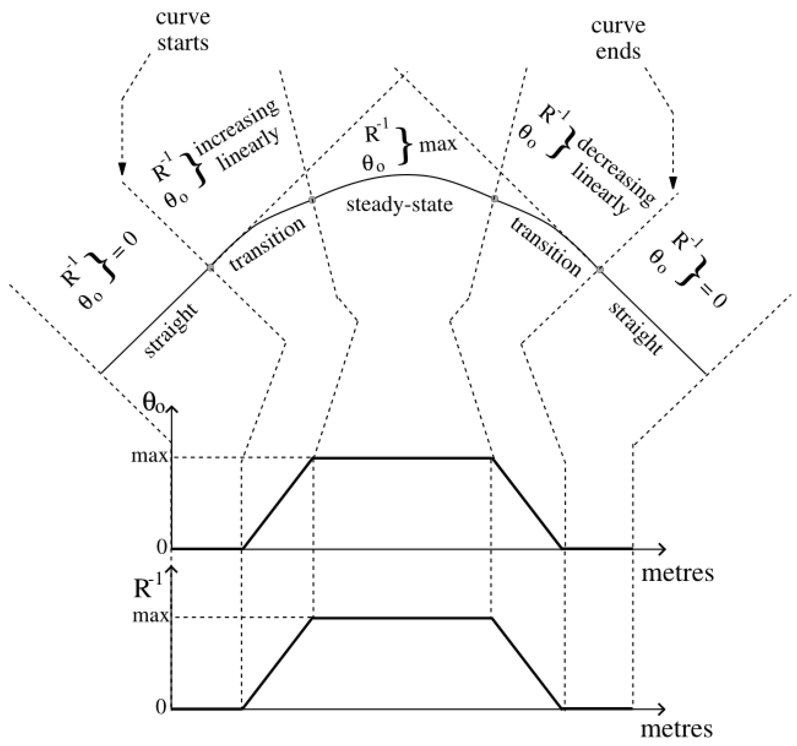
The intended geometrical layout of the rail track is where the deterministic track (curved track disturbance) originates. Civil engineers created this to make sure that it will have the desired impact on passenger comfort. Notably, the deterministic track in tilting trains relates to curved sections of the track segments with measurable curvature ( R 1 , R being the curve radius from a virtual inwards curve centre). In order to minimize the effect of the centrifugal forces felt by the passenger, the track was canted to rotate the vehicle inwards. During the curve transitions, the rates of cant and curvature change linearly but settle on a steady-state curve; refer to Figure 2.
The misalignment dominant spectral characteristics of the lateral track position variable appear at a higher frequency compared to the deterministic input characteristics (but not high enough to be considered completely decoupled). Additionally, the ideal tilt action command is provided by the control input (processed via the actuator servo). For more details, the reader is referred to [9,23].
For simulation and assessment purposes, the track profiles with 60% tilt compensation for curved and straight track irregularities can be found in Table 1.

2.2. Non-Minimum Phase System Arising from Non-Preview Tilt

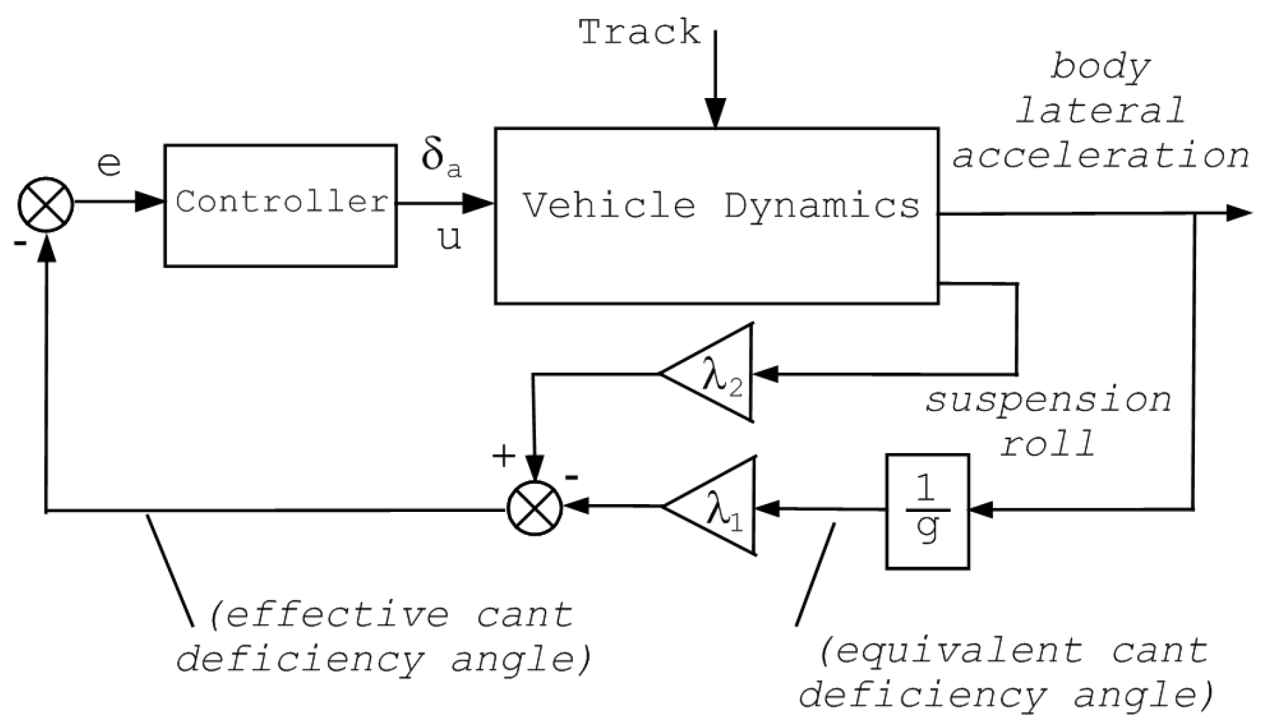
Early tilt control design tried to satisfy the full passenger lateral acceleration on a curved track, which proved unsuccessful from a passenger motion sickness perspective [8,23]. Hence, only a portion of tilt was compensated for and the solution was labeled “partial-tilt compensation”. This partial-tilt scheme compensation within 60–75% (of lateral acceleration on a steady curve) is provided by the measured acceleration signal and vehicle body roll angle (tilt). This scheme feedback control setup is presented in Figure 3.
The output signal used for feedback control is the so-called effective cant deficiency (which forces the partial-tilt compensation) given by
θ d m = λ 1 y ¨ v m g + λ 2 θ 2 s r
where y ¨ v m is the passengers’ perceived lateral acceleration, as determined by an accelerometer on the body c.o.g (6), and θ 2 s r is the secondary suspension roll angle (7).
y ¨ v m = v 2 R g θ o + θ v + y ¨ v
θ 2 s r = θ v θ b
The parameters λ 1 ,   λ 2 in this work were selected to provide 60% tilt compensation on a steady-state curve (i.e., λ 1 = 0.6 ,   λ 2 = 0.4 , respectively, if bogie roll-out is neglected). Note that, in practice, due to the stiff primary suspensions, the bogie roll-out only has a limited effect and can be safely neglected for control design purposes.
From a control-theoretic point of view, the scheme represents a typical single-input–single-output (SISO) structure. The design (nominal) model transfer function is given by (8). The full mathematical modeling of this transfer function representative can be found in [22].
The nominal model transfer function in (8) represents the dynamic relationship between the output Y ( e . c . d ) and the control input Δ ( t i ) .
Where Y ( e . c . d ) is the 60% compensation effective cant deficiency and Δ ( t i ) is the ideal control tilt angle.
Y e c d ( s ) Δ t i ( s ) = N t ( s ) D t ( s )
The numerator of the transfer function is given by
N t ( s ) = 27531 ( s 29.36 ) ( s 6.02 ) ( s 2 + 66.91 s + 1066 ) ( s 2 + 7.65 s + 24.44 )
and the denominator
D t ( s ) = ( s + 23.2 ) ( s 2 + 1.38 s + 17.44 ) ( s 2 + 5.11 s + 88 ) ( s 2 + 22 s + 483.6 ) ( s 2 + 29.15 s + 4.9 e 3 ) ( s 2 + 4.83 s + 15.9 e 3 ) ( s 2 + 41.73 s + 28.4 e 3 )
The above transfer function refers to the nominal model.
An important point is that the non-preview tilt approach suffers from control bandwidth constraints due to the existence of non-minimum phase (NMP) zeros in numerator N t ( s ) . These arise due to the location of the suspensions (and the suspension interactions), relative to the centre of gravity and the center of tilt, and the roll angle contribution (from a portion of the gravitational force) measured by the lateral accelerometer. More details on the exact nature of such NMP zeros can be found in [16] and other applications in [24,25].

2.3. Parametric Uncertainty Information

Prior to discussing the approach of setting up the design models for control, we present realistic uncertainty of the vehicle parameters. Four plant perturbations (in addition to the nominal model) were chosen. Table 2 presents the uncertainty details (the variation is relative the nominal model); note that the nominal model is denoted as ‘P0’.

2.4. Design Models for Control

Three alternative plant families are proposed here regarding the modeling for control. As mentioned earlier in the vehicle modeling, the nominal transfer function G p ( s ) = N t ( s ) / D t ( s ) includes a pair of NMP zeros. We present the three representations in a rather developmental way, useful for enabling a better understanding of the level of robust control design in the sequence.
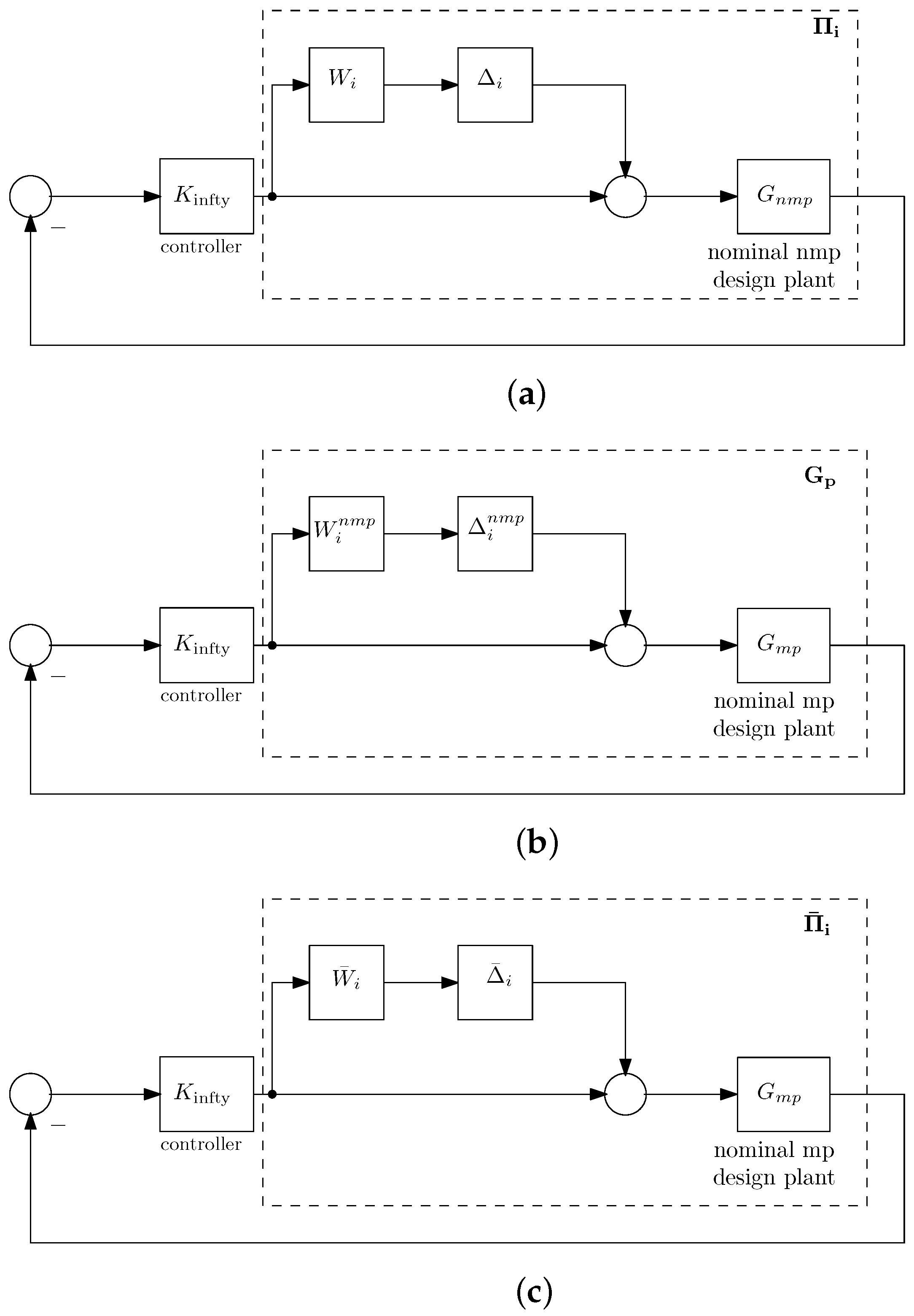
Π i : G p p ( s ) = G p ( s ) 1 + W i ( s ) Δ i ( s )
G p : G p ( s ) = G m p ( s ) 1 + W Δ u z ( s ) Δ u z ( s )
Π ¯ i : G ¯ p p ( s ) = G m p ( s ) 1 + W ¯ i ( s ) Δ ¯ i ( s )
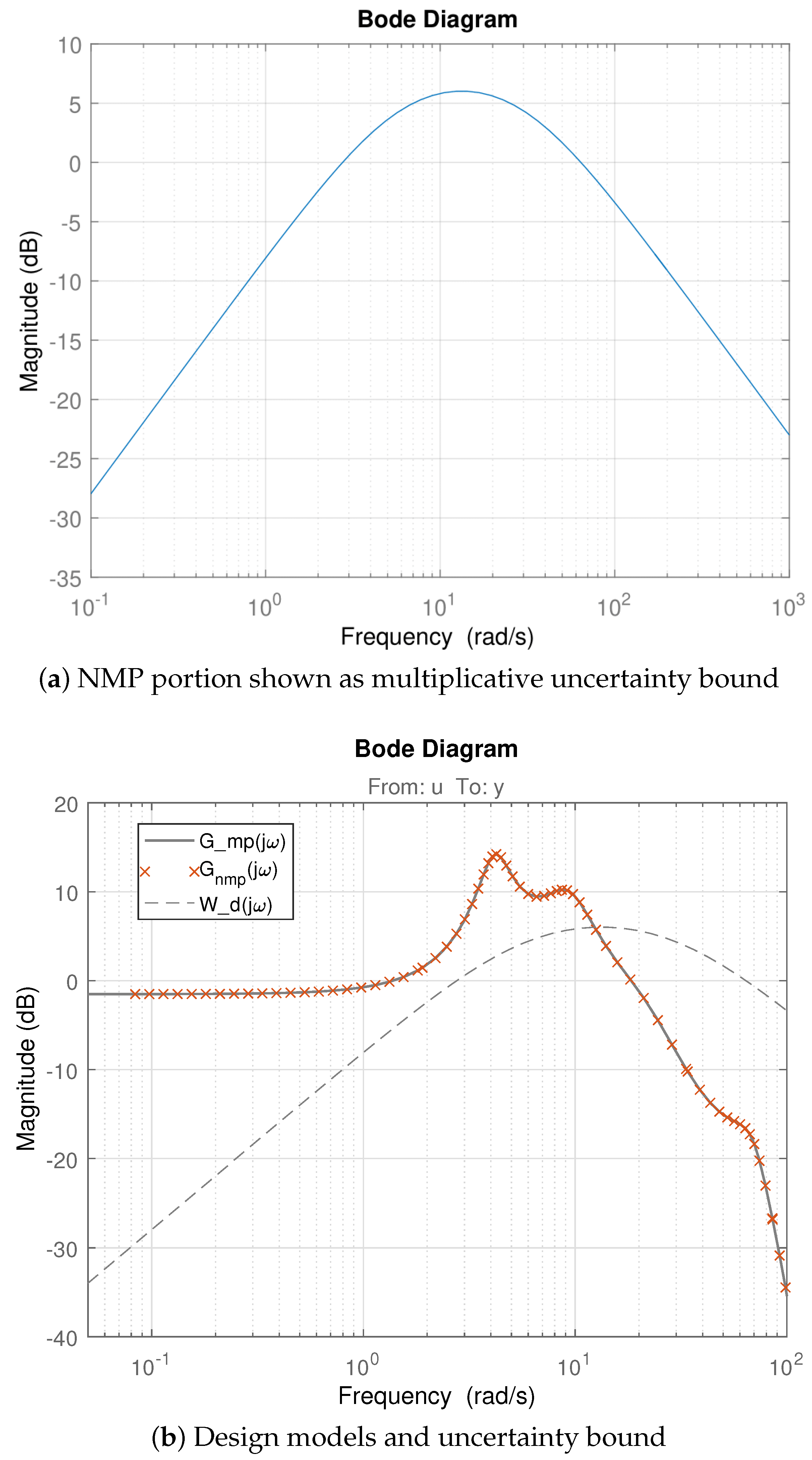
The first representation, i.e., Π i , comprises the parametric uncertainty in the form of multiplicative uncertainty (the nominal model is the one that includes the NMP zeros). The second representation G p presents a factorized model form whereby the NMP zeros are mapped into equivalent multiplicative uncertainty (the virtual nominal plant here includes only the minimum-phase portion, i.e., labeled G mp ( s ) ). The frequency response for both models are illustrated in Figure 4. The third representation Π ¯ i presents a factorized model whereby both the parametric uncertainty and the NMP zeros are included in a bulk multiplicative uncertainty form (again, the virtual nominal plant here includes only the minimum-phase portion, i.e., labeled G mp ( s ) ). The reason for proposing the above representations is rather straightforward and essentially addresses the way that the choice of the uncertainty formulation impacts robust control design in the non-preview tilt (in fact, the multiplicative uncertainty weight enters robust stability considerations). In this context, note that Π i is the normal representation that a designer would employ in a robust H-infinity mixed sensitivity design, and G p facilitates exploring whether the conservativeness of mapping NMP zeros into multiplicative uncertainty provides a good enough solution (without considering further uncertainty in the first instance). Π ¯ i represents the most conservative representation (with the overall bulk uncertainty form).
Here, we looked into the way to factorize the nominal model into a minimum phase (MP where no non-minimum-phase zeros are included) and the non-minimum-phase zeros as multiplicative uncertainty bound. The feedback setup for this multiplicative uncertainty model can be seen in Figure 5a–c.
The transfer function plant G ( s ) in Equation (12) can be rearranged as
G ( s ) = G m p ( s ) G a l l p ( s )
G a l l p ( s ) is an all-pass transfer function (comprising the NMP zeros) and can be expressed in the form of multiplicative uncertainty, as in (12), directly.
Recall that Δ (s) is any stable transfer function where Δ ( j ω ) 1 .
W Δ ( j ω ) = j 70.76 ω ( 176.7 ω 2 ) + j 35.38 ω
The magnitude plot of this particular case of multiplicative uncertainty bound covers the NMP zeros of the system and is presented in Figure 6.
The design approach introduces some conservativeness by representing the NMP zeros as multiplicative uncertainty (nominal), G m p ( s ) .
Note that the two NMP zero frequencies’ bandpasses are where the uncertainty is located.

3. Robust Control Design

The tuning of weighting functions in the H mixed-sensitivity controller in the optimization process was implemented using fmincon() in MATLAB.
The optimized minimization problem by imposing ride quality degradation as a constraint is given by
minimize W 1 W 2 f ( x ) = P C T s t a n d i n g subject to < constraint = rqd 7 . 5 % >
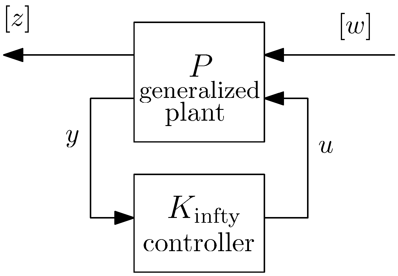
The design problem regarding obtaining a model-based controller K i n f t y ( s ) is presented in Figure 7. This presented framework is designed to meet several control requirements, such as closed loop stability, a good tracking or disturbance rejection performance, and robust stability in the presence of modeling uncertainties in the model. Here, H mixed sensitivity was applied on both NMP plant transfer function ( G p ) and the MP factorized transfer function ( G m p ), which is different to what was addressed in [21]. The multiplicative uncertainty bound for the complementary sensitivity, T, has already been obtained for the G m p case.
The nonlinear optimization via different weighted choices is presented in Table 3 and Table 4. For P 2 x N M P and P 2 x M P cases in Table 4, only W1 is obtained via optimization while W 2 and W 3 are fixed. W 3 is W δ for the NMP (nominal plant G p ) model case and W δ M P for the MP (factorized plant ( G m p )) model.
The sensitivity frequency weight, W 1 , in Equation (17)’s second-order transfer function formula was introduced by [26]. W B * represents the maximum frequency bandwidth, M is the maximum peak of sensitivity ( S ( j ω ) ), and A is the maximum steady-state tracking error.
The initial value for W 1 parameters was obtained from the PID design in [15]. The upper and lower bound W 1 parameter value for both the NMP and MP model was chosen to be a decade above and lower for optimization purposes.
W 1 = ( s / ( M ( 1 / 2 ) ) + W B ) 2 ( s + W B ( A ) ( 1 / 2 ) ) 2
The expected range of W 2 in all cases (initial values and fixed level values) was obtained via previous work in [15]. Four (4) cases with different values of fixed W 2 and W 3 for both P x 2 N M P and P x 2 M P are presented in Table 4. The values of W 2 used here are 0.75, 0.5, 0.1, and a high-pass filter, respectively, and W 3 is W δ . Keep in mind that W 2 was used as a high-pass filter introduced here for completeness following the work by [21].

4. Nominal Performance Analysis

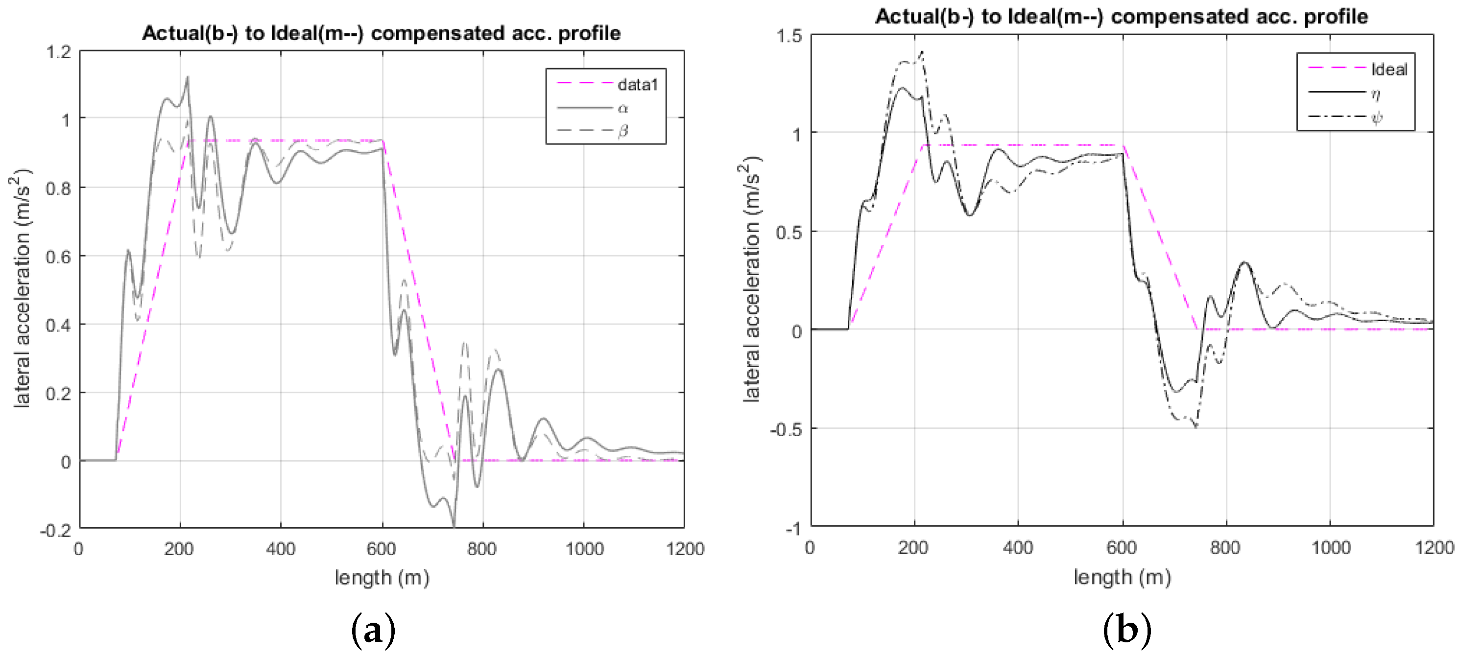
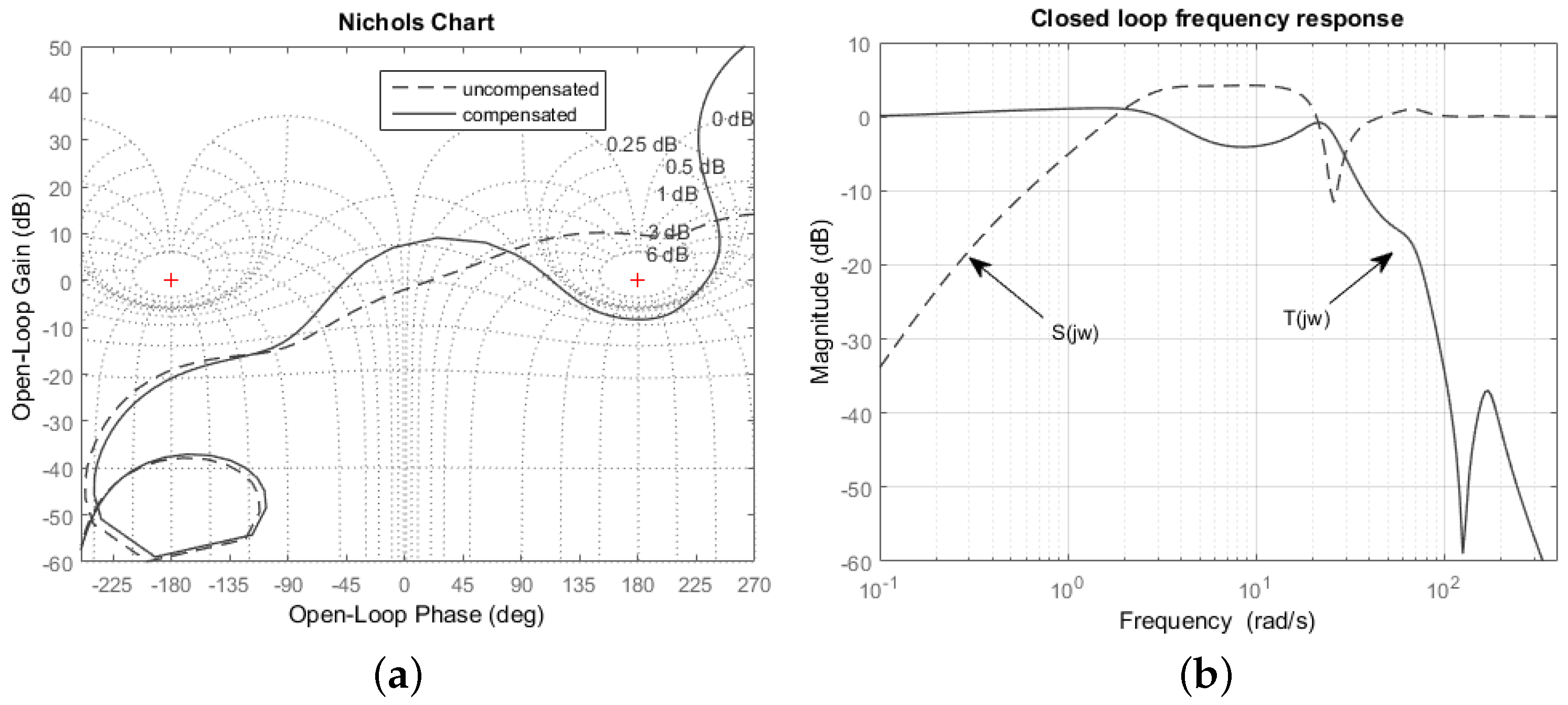
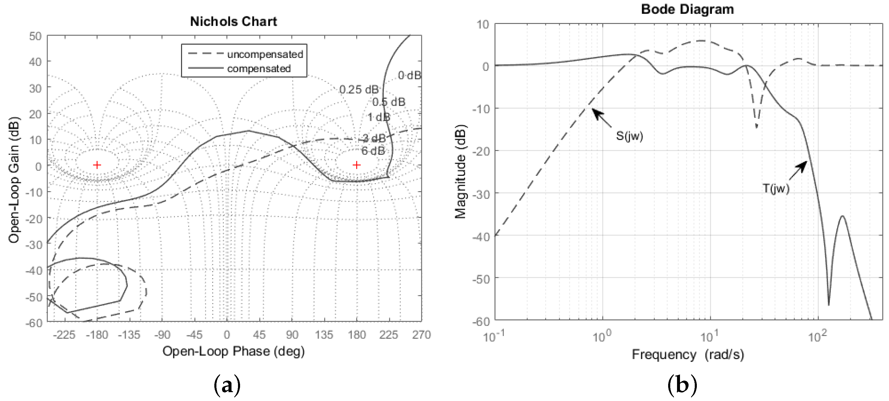
The full-order H mixed-sensitivity controller performance on the nominal model for P 1 N M P , P 2 N M P , P 1 M P , and P 2 M P is presented in Table 5. The table clearly demonstrates how the design is progressing and how the conservatism induced by taking the MP plant into consideration, together with the related uncertainty, affects the design. In fact, the results for the NMP plant are significantly better than the previous analysis presented in [21]. Time-domain lateral acceleration plot responses can be seen in Figure 8. The conservatism of the MP model designed as compare with NMP model can also be proven in the frequency plot in Figure 9, Figure 10, Figure 11 and Figure 12.
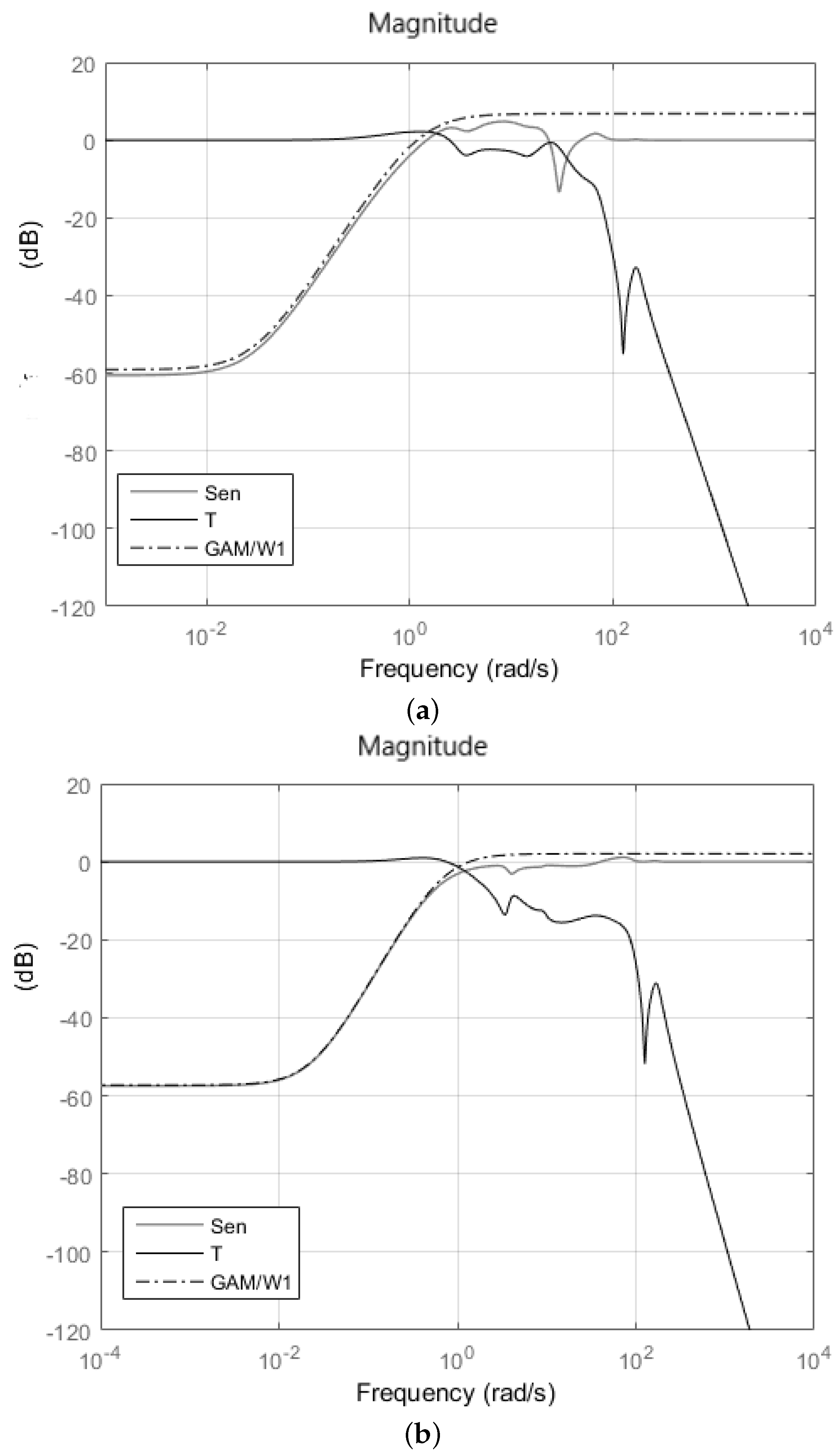
Table 6 and Table 7 show the result for the nominal performance of P x 2 N M P (NMP case) and P x 2 M P (MP case), respectively. A value of ride quality trade-off below 7.5 can be achieved with W 2 values of 0.75 and 0.5. The controller design with MP cases, however, shows a much higher P C T performance resulting from imposing extra conservativeness on the MP model. This is proven from the sensitivity plot shown in Figure 13 for the P x 2 N M P W 2 = 0.5 and P x 2 M P W 2 = 0.1 case. P x 2 M P W 2 = 0.1 shows a very narrow gap between S ( j w ) and γ / W 1 in Figure 13.
The tilt performance for fixed W 2 for the remaining system identifiers P x 2 N M P , P x 2 M P is presented in Table 6 and Table 7. The proposed robust design for this case shows that the best result is obtained from the NMP case, though the MP case gives a consistent tilt performance.
From the control theoretical point of view, if the γ values obtained are larger than 1, the desired specification in the stacked requirements is not precisely realized. However, it is not a crucial point in this case since the controller design in the optimization process presented in this paper prioritized the tilt control performance rather than just the obtained value of γ . For completeness, sensitivity plots with respect to γ / W 1 are illustrated in Figure 13.

Controller Reduction and Robust Performance Investigation

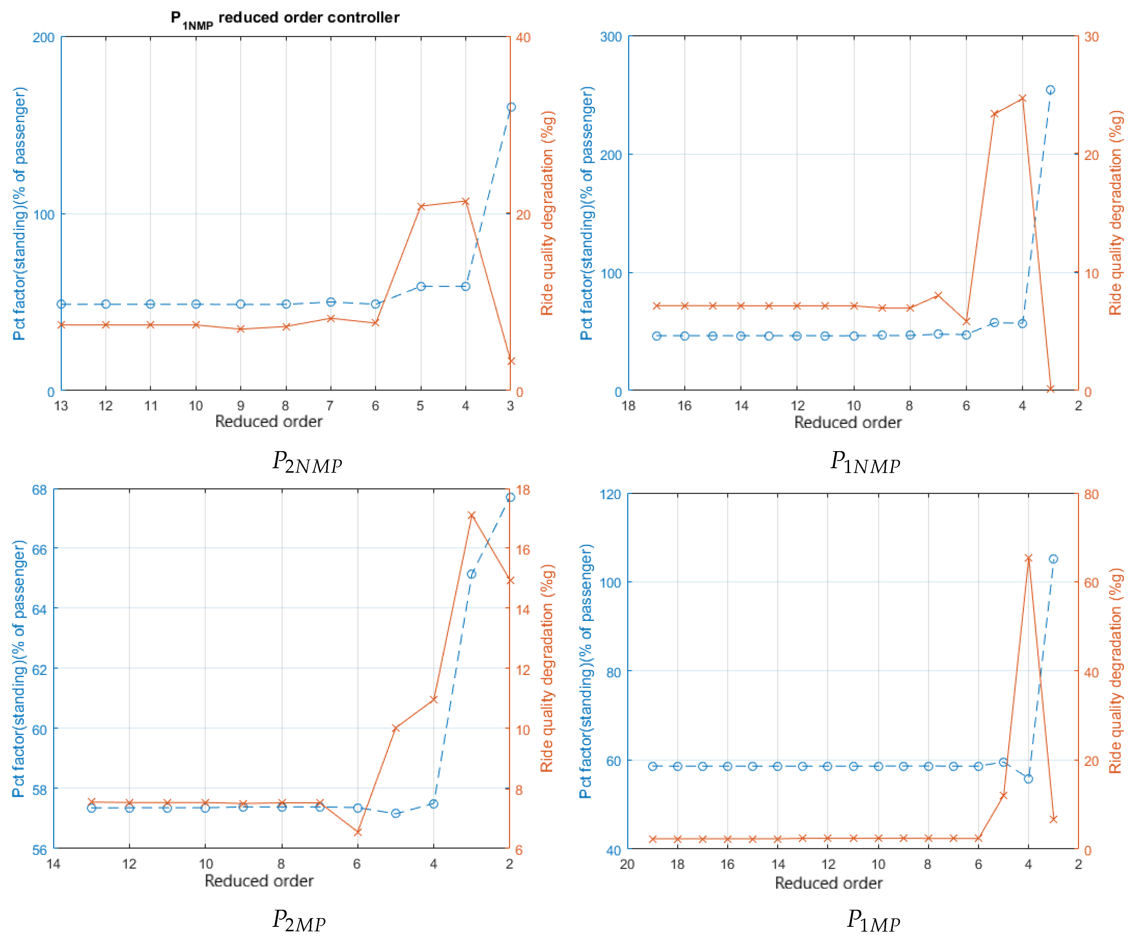
Since the H controllers used here were model-based, the controller order achieved from the optimization design tended to be large (can be up to 18th order in this case and differs for each case). Following the same controller reduction method as that presented in [15], we briefly provide controller reduction results here. It can be concluded from Figure 14 that the P C T and ride quality performance trade-off are still maintained up to a seventh-order reduction for all cases.
The controller must meet both nominal and robust stability requirements in order to guarantee the robustness of the system’s performance. Note that, in order to achieve the control specifications, one should strictly talk about performance rather than just stability—though here we only refer to bounds for stability. We offer a straightforward method for expressing multiplicative uncertainty as the parametric uncertainty on the actual design transfer function (including NMP zeros). While the case in the previous Section 4 was easily obtained analytically, here, the bound was obtained in the form of an envelope covering a wide range of frequency responses.
Here, four choices of plant perturbation, including nominal plant P 0 , were used for robust performance analysis, i.e., refer to Table 2.
We offer a succinct discussion on robust performance based on the reduced controllers that were produced. The reduced controller order used for robust performance analysis here was the eighth order based on the analysis performed in Figure 14. In addition, note that only six (6) “best” cases are presented here.
The results of the eighth-reduced-order controller on the robust tilt performance of for all six cases are given in Table 8 and Table 9. It can be said that, for all chosen cases, the P C T factor performance is maintained for all four (4) plant uncertainty cases of P 1 , P 2 , P 3 , and P 4 . The worst ride quality degradation is maintained below 15 % for all three MP models ( P 1 M P , P 2 M P , and P 2 x M P ) on the P 1 , P 2 , and P 3 plant due to the extra conservativeness of the MP model. However, the MP model P 1 M P cannot maintain a below 15 % worst ride quality degradation performance for the P 4 uncertainty plant. In fact, P 4 is the worst plant uncertainty case since the NMP model shows an unstable performance on this plant. Although the robustness of more conservative controller designs tends to be better, they may fall short of the expected improvement in nulling-type tilt control performance (which should be as close as possible to the performance provided by a tilt with a precedence equivalent).
The results obtained (for the nominal models) via this proposed robust controller approach compared to the ones obtained by [21] are much improved (esp. the PCT factor for P 2 x N M P 0.5 , P 2 N M , P 1 N M P ; note that the ride quality is a constraint, i.e., should be ≤7.5%, and is not the primary concern to optimize: the deterministic response is the primary point to address and optimize). Note that the best PCT obtained in [21] is approx. 51.7 % . In addition, the work in this paper studied the robust performance in detail. Similar conclusions can be drawn comparing the results to the ones obtained in [22] (PCT obtained is approx. 62 % ). A direct comparison is possible as the track excitation input (deterministic, stochastic) is the same in all cases.

5. Conclusions

This paper rigorously studied optimized H mixed sensitivity in tilt control design in the context of a single-input–single-output control framework. In particular, the impact of the proposed controller in a nominal and multiplicative uncertainty plant of both an MP and NMP model was presented and compared. The detailed nominal and robust performance of H mixed sensitivity in both a nominal and multiplicative uncertainty plant was illustrated via simulation results. The robust controller design was followed via a twofold method: (i) using the non-minimum phase design model and (ii) proposing a factorized design model version with the non-minimum phase characteristics treated as uncertainty. Rigorous analysis provided useful insights in selecting the best tilt controller to obtain a trade-off between the nominal performance and robust performance. While this work addressed tilt control design, the proposed approach can be applied to active suspension of a similar nature and other applications exhibiting non-minimum phase characteristics in their representative model.

Author Contributions

Conceptualization, F.H. and A.Z.; writing—original draft, F.H.; formal analysis, F.H.; supervision, A.Z.; validation, F.H.; writing—reviewing and editing, F.H., A.Z. and G.H.; investigation, F.H.; visualization, F.H.; resources, F.H., A.Z. and G.H.; methodology, F.H.; software, F.H. All authors have read and agreed to the published version of the manuscript.

Funding

This research was funded by the Ministry of Education Malaysia under Fundamental Research Grant Scheme (FRGS).

Data Availability Statement

Results can be duplicated directly from data information provided in the article. Data sharing is not applicable to this article.

Acknowledgments

The authors would like to acknowledge the financial support from the Ministry of Education Malaysia under Fundamental Research Grant Scheme(FRGS) FRGS/1/2019/TK08/UTM/02/3.

Conflicts of Interest

The authors declare no conflict of interest.

Abbreviations

The following abbreviations are used in this manuscript:
GPSGlobal Positioning System
SISOSingle-Input–Single-Output
NMPNon-Minimum Phase
MPMinimum Phase
PIDProportional Integral Derivative
TFTransfer Function

Appendix A. Variables and Parameters List

y v , y b , y 0 Lateral displacement of body, bogie, and railtrack (m)
y v ˙ , y b ˙ , y 0 ˙ Roll rate of body, bogie, and railtrack (m/s)
θ v , θ b Roll displacement of body, bogie, and actuator (rad)
δ t , δ t ˙ Applied tilt (rad) and tilt rate (rad/s)
R 1 , R 1 ˙ Curve radius rate and acceleration
θ 0 Rail track cant, curve radius (rad)
θ r Airspring reservoir roll deflection (rad)
vVehicle forward speed (tilting: 58 m/s)
m v Half body mass, 19,000 (kg)
i vr Half body inertia, 25,000 (kgm)
m b Bogie mass, 2500 (kg)
i b r Bogie roll inertia, 1500 (kgm 2 )
k a z Airspring area stiffness, 210 × 10 3 N/m
k s z Airspring series stiffness, 620 × 10 3 N/m
k r z Airspring reservoir stiffness, 244 × 10 3 N/m
c r z Airspring reservoir damping, 33 × 10 3 Ns/m
k s y Secondary lateral stiffness, 260 × 10 3 N/m
c s y Secondary lateral damping, 33 × 10 3 Ns/m
y w , y w ˙ Bogie kinematics position (m), rate (m/s)

References

  1. Iwnicki, S. Handbook of Railway Vehicle Dynamics; CRC Press: Boca Raton, FL, USA, 2006. [Google Scholar]
  2. Vickerman, R. High-speed rail in Europe: Experience and issues for future development. Ann. Reg. Sci. 1997, 31, 21–38. [Google Scholar] [CrossRef]
  3. Fröidh, O. Perspectives for a future high-speed train in the Swedish domestic travel market. J. Transp. Geogr. 2008, 16, 268–277. [Google Scholar] [CrossRef]
  4. Darlton, A.O.; Marinov, M. Suitability of tilting technology to the tyne and wear metro system. Urban Rail Transit 2015, 1, 47–68. [Google Scholar] [CrossRef] [Green Version]
  5. Stribersky, A.; Steidl, S.; Müller, H.; Rath, B. On dynamic analyses of rail vehicles with electronically controlled suspensions. Veh. Syst. Dyn. 1996, 25, 614–628. [Google Scholar] [CrossRef]
  6. Pearson, J.T.; Goodall, R.M.; Pratt, I. Control system studies of an active anti-roll bar tilt system for railway vehicles. Proc. Inst. Mech. Eng. Part J. Rail Rapid Transit 1998, 212, 43–60. [Google Scholar] [CrossRef]
  7. Huber, B.H. The bogie-based tilt option-simplicity and flexibility. Proc. Inst. Mech. Eng. Part J. Rail Rapid Transit 1998, 212, 19–32. [Google Scholar] [CrossRef]
  8. Persson, R.; Goodall, R.M.; Sasaki, K. Carbody tilting–technologies and benefits. Veh. Syst. Dyn. 2009, 47, 949–981. [Google Scholar] [CrossRef] [Green Version]
  9. Zolotas, A.; Goodall, R.M.; Halikias, G.D. New control strategies for tilting trains. Veh. Syst. Dyn. 2002, 37, 171–182. [Google Scholar] [CrossRef] [Green Version]
  10. Bruni, S.; Goodall, R.; Mei, T.X.; Tsunashima, H. Control and monitoring for railway vehicle dynamics. Veh. Syst. Dyn. 2007, 45, 743–779. [Google Scholar] [CrossRef]
  11. Hohenbichler, N.; Six, K.; Abel, D. The Benefit of Skyhook control in high speed railway vehicles. Ifac Proc. Vol. 2006, 39, 890–895. [Google Scholar] [CrossRef]
  12. Zhao, Y.; Wang, T.; Karimi, H.R. Distributed cruise control of high-speed trains. J. Frankl. Inst. 2017, 354, 6044–6061. [Google Scholar] [CrossRef]
  13. Ye, J.; Sun, H. The Influence of an Integration Time Step on Dynamic Calculation of a Vehicle-Track-Bridge under High-Speed Railway. Math. Digit. Publ. Inst. 2021, 9, 431. [Google Scholar] [CrossRef]
  14. Zamzuri, H.; Zolotas, A.C.; Goodall, R.M. Tilt control design for high-speed trains: A study on multi-objective tuning approaches. Veh. Syst. Dyn. 2008, 46, 535–547. [Google Scholar] [CrossRef] [Green Version]
  15. Hassan, F.; Zolotas, A.C.; Margetts, R. Improved PID control for tilting trains. In Proceedings of the 2016 IEEE International Conference for Students on Applied Engineering (ICSAE), Newcastle Upon Tyne, UK, 20–21 October 2016. [Google Scholar]
  16. Hassan, F.; Zolotas, A. Impact of fractional order methods on optimized tilt control for rail vehicles. Fract. Calc. Appl. Anal. 2017, 20, 765–789. [Google Scholar] [CrossRef]
  17. Chaudhuri, B.; Pal, B.C.; Zolotas, A.C.; Jaimoukha, I.M.; Green, T.C. Mixed-sensitivity approach to H∞ control of power system oscillations employing multiple FACTS devices. IEEE Trans. Power Syst. 2003, 18, 1149–1156. [Google Scholar] [CrossRef] [Green Version]
  18. Fales, R.; Kelkar, A. Robust control design for a wheel loader using mixed sensitivity H-infinity and feedback linearization based methods. In Proceedings of the 2005, American Control Conference, Portland, OR, USA, 8–10 June 2005; pp. 4381–4386. [Google Scholar]
  19. Bakouri, M.; Alassaf, A.; Alshareef, K.; Abdelsalam, S.; Ismail, H.F.; Ganoun, A.; Alomari, A.-H. An Optimal H-Infinity Controller for Left Ventricular Assist Devices Based on a Starling-like Controller: A Simulation Study. Mathematics 2022, 10, 731. [Google Scholar] [CrossRef]
  20. Yan, S.-R.; Alattas, K.A.; Bakouri, M.; Alanazi, A.K.; Mohammadzadeh, A.; Mobayen, S.; Zhilenkov, A.; Guo, W. Generalized Type-2 Fuzzy Control for Type-I Diabetes: Analytical Robust System. Mathematics 2022, 10, 690. [Google Scholar] [CrossRef]
  21. Zolotas, A.C. Advanced Control Strategies for Tilting Trains. Ph.D. Thesis, Loughborough University, Loughborough, UK, 2002. [Google Scholar]
  22. Zolotas, A.C.; Wang, J.; Goodall, R.M. Reduced-order robust tilt control design for high-speed railway vehicles. Veh. Syst. Dyn. 2008, 46, 995–1011. [Google Scholar] [CrossRef] [Green Version]
  23. Zolotas, A.C.; Goodall, R.M. Advanced control strategies for tilting railway vehicles. In UKACC International Conference on Control; University of Cambridge: Cambridge, UK, 2000. [Google Scholar]
  24. Al-Baidhani, H.; Sahib, A.; Kazimierczuk, M.K. State Feedback with Integral Control Circuit Design of DC-DC Buck-Boost Converter. Mathematics 2023, 11, 2139. [Google Scholar] [CrossRef]
  25. Ivanov, D.; Granichin, O.; Pankov, V.; Volkovich, Z. Design of 1 New Suboptimal Fractional Delays Controller for Discrete Non-Minimum Phase System under Unknown-but-Bounded Disturbance. Mathematics 2022, 10, 69. [Google Scholar] [CrossRef]
  26. Skogestad, S.; Postlethwaite, I. Multivariable Feedback Control: Analysis and Design; Wiley: Hoboken, NJ, USA, 2007; Volume 2. [Google Scholar]
Figure 1. End-view of the tilting vehicle structure.
Mathematics 11 03057 g001
Figure 2. Deterministic track profile representation.
Mathematics 11 03057 g002
Figure 3. Partial nulling tilt compensation control feedback setup.
Mathematics 11 03057 g003
Figure 4. Frequency response of NMP original and of MP factorized TFs.
Mathematics 11 03057 g004
Figure 5. Feedback setup with multiplicative uncertainty. (a) The plant family Π i for the NMP system model. (b) The factorized nominal NMP model. (c) The overall uncertainty control feedback setup for nominal minimum phase (MP) model.
Mathematics 11 03057 g005
Figure 6. Consideration of model factorization.
Mathematics 11 03057 g006
Figure 7. Generalized regulator setup for the H mixed-sensitivity design.
Mathematics 11 03057 g007
Figure 8. Lateral acceleration plot for P 1 N M P -( α ) and P 2 N M P ( β ) (a), P 1 M P ( η ) and P 2 M P ( ψ ) (b).
Mathematics 11 03057 g008
Figure 9. Open loop (a) and closed loop (b) complementary sensitivity ( T ( j ω ) ) and sensitivity ( S ( j ω ) ) plots for P 1 N M P case.
Mathematics 11 03057 g009
Figure 10. Open loop (a) and closed loop (b) complementary sensitivity ( T ( j ω ) ) and sensitivity ( S ( j ω ) ) plots for P 2 N M P case.
Mathematics 11 03057 g010
Figure 11. Open loop (a) and closed loop (b) complementary sensitivity ( T ( j ω ) ) and sensitivity( S ( j ω ) ) plots for P 1 M P case.
Mathematics 11 03057 g011
Figure 12. Open loop (a) and closed loop (b) complementary sensitivity ( T ( j ω ) ) and sensitivity ( S ( j ω ) ) plots for P 2 M P case.
Mathematics 11 03057 g012
Figure 13. Sensitivity (S), complementary sensitivity (T), and γ / W 1 plot for (a) P x 2 N M P W 2 = 0.5 ; (b) P x 2 M P W 2 = 0.1 .
Mathematics 11 03057 g013
Figure 14. Controller reduction and performance trade-off for H mixed-sensitivity cases. The blue line represents P C T factor of standing passenger, the red line represents ride quality degradation.
Mathematics 11 03057 g014
Table 1. The track test profiles used for simulation and assessment.
Tilt Compensation60%Units
deterministic (curved track)
maximum cant angle θ o { max } 6.00(degrees)
maximum curve radius R max 1000.00(m)
transition length 145.00(m) @ each end
track length 1200.00(m)
stochastic (straight track)
track roughness Ω l 0.33 × 10 8 (m)
track spatial spectrum S T Ω l / f 3 m 2 ( cycle / m )
track length 1200.00(m)
Table 2. Perturbed (uncertainty) plant cases.
Plant IDPerturbation
P1 20 % body mass increase
P2 20 % body mass decrease
P3 20 % decrease in dynamic body mass and 40 % ( 20 % ) decrease (increase) in secondary suspension damping (stiffness)
P4 20 % increase in dynamic body mass and 30 % ( 20 % ) decrease (increase) in secondary suspension stiffness (damping)
Table 3. Minimization approach identifiers and weight sensitivity parameters (transfer function) for H mixed-sensitivity optimization (note: rqd denotes ride quality degradation).
Minimization ID W 1 W 2 W 3
P 1 N M P s 2 + 1.317 s + 0.4337 1.255 s 2 + 0.06102 s + 0.0007416 0.9355not used
P 2 N M P s 2 + 3.06 s + 2.341 2 s 2 + 0.1374 s + 0.00236 0.7047 W δ
P 1 M P s 2 + 0.8792 s + 0.1932 1.311 s 2 + 0.03184 s + 0.0001933 0.5338not used
P 2 M P s 2 + 1.063 s + 0.2823 2 s 2 + 0.06721 s + 0.0005646 0.309 W δ M P
Table 4. Minimization approach identifiers and weight sensitivity parameters (transfer function) for H mixed-sensitivity optimization for P x 2 N M P and P x 2 M P with fixed W 2 and W 3 (note: rqd denotes ride quality degradation).
W 2 NMP W 1 NMP W 2 MP W 1 MP
W2 = 0.75 s 2 + 3.033 s + 2.3 2 s 2 + 0.1356 s + 0.0023 W2 = 0.5 s 2 + 0.972 s + 0.2362 1.2 s 2 + 0.03367 s + 0.0002362
W2 = 0.5 s 2 + 2.579 s + 1.663 1.972 s 2 + 0.1145 s + 0.001663 W2 = 0.1 s 2 + 1.4 s + 0.4899 1.813 s 2 + 0.08429 s + 0.0009799
W2 = 0.1 s 2 + 0.818 s + 0.1673 2 s 2 + 0.0413 s + 0.000213 W2 = 0.05 s 2 + 1.407 s + 0.4949 1.851 s 2 + 0.08562 s + 0.0009898
W 2 h p f s 2 + 2.219 s + 1.231 1.212 s 2 + 0.09887 s + 0.002016   
Table 5. H Mixed-sensitivity controller performance assessment with the different time-domain optimization approaches.
Deterministic (as Per Given Units) P 1 NMP P 2 NMP P 1 MP P 2 MP
Lateral accel.RMS deviation (%g)2.1942.0642.9213.474
Peak value (%g)11.43410.13712.47614.388
Roll gyro.RMS deviation (rad/s)0.0240.0240.0310.033
Peak value (rad/s)0.1180.1240.1270.114
P C T -relatedPeak jerk level (%g/s)6.4956.2798.0257.933
Standing (% of passenger)48.70346.4157.35958.672
Seated (% of passenger)13.02911.91215.73716.832
Stochastic(acceleration %g) @58 m/s 1
Ride qualityTilting train3.0593.0523.0632.914
Degradation (%)7.4137.1667.552.331
Performance Margins
Freq. resp.Gain margin (dB)8.3066.2438.47510.607
Phase margin (deg)52.68244.51341.08357.123
Bandwidth (rad/s)1.251.230.8090.723
S ( j ω ) 1.6251.9521.9931.535
Gamma γ 1.31391.32210.84090.6412
1 Ride quality for non-tilting train if running at the higher speed = 2.848 % g.
Table 6. H Mixed-sensitivity controller performance assessment with the different fixed W 2 values for P x 2 N M P case.
Deterministic W 2 W 2 W 2 W 2
(as per Given Units)0.750.50.1HPF
P C T -relatedPeak jerk level (% g/s)6.296.6749.0047.140
Standing (% of passenger)46.34148.70666.04552.106
Seated (% of passenger)11.90212.78620.13814.124
Stochastic (acceleration %g) @58 m/s 1
Ride qualityTilting train3.0563.0323.0622.957
Degradation (%)7.3066.4627.523.840
Performance Margins
Freq. resp.Gain margin (dB)6.1427.48415.8588.540
Phase margin (deg)44.1948.26365.45752.718
S ( j ω ) 1.9741.7361.1951.596
Gamma γ 1.2941.1120.6231.446
1 Ride quality for non-tilting train if running at the higher speed = 2.848 % g.
Table 7. H Mixed-sensitivity controller performance assessment with the different fixed W 2 values for P x 2 M P case.
Deterministic W 2 W 2 W 2
(as per Given Units)0.50.10.05
P C T -relatedPeak jerk level (% g/s)7.6477.6387.671
Standing (% of passenger)56.88456.45156.595
Seated (% of passenger)15.96415.89715.973
Stochastic (acceleration %g) @58 m/s 1
Ride qualityTilting train3.0622.9613.022
Degradation (%)7.4973.9716.120
Performance Margins
Freq. resp.Gain margin (dB)8.68910.29910.508
Phase margin (deg)55.33955.30755.538
S ( j ω ) 1.8271.5851.559
Gamma γ 0.91300.68690.6752
1 Ride quality for non-tilting train if running at the higher speed = 2.848 % g.
Table 8. Robust performance for P C T standing for 8th-order H controller.
CaseP0 NominalP1P2P3P4
P 1 N M P 48.67449.96550.26450.60651.688
P 2 N M P 46.53546.19648.95757.20047.904
P 2 x N M P 0.5 48.81649.58349.91050.23050.662
P 1 M P 57.39259.56755.36255.57163.388
P 2 M P 58.68262.16159.94360.86065.678
P 2 x M P 0.1 56.66759.83158.94459.76563.196
Table 9. Robust performance for ride quality for 8th-order H controller.
CaseP0 NominalP1P2P3P4
P 1 N M P 7.24129.45314.53936.730unstable
P 2 N M P 6.96624.41822.47592.808unstable
P 2 x N M P 0.5 6.21015.50917.37935.49769.424
P 1 M P 7.52714.2884.5814.16829.282
P 2 M P 2.4035.866−0.481−1.25310.002
P 2 x M P 0.1 4.3727.6922.6982.13713.244
Disclaimer/Publisher’s Note: The statements, opinions and data contained in all publications are solely those of the individual author(s) and contributor(s) and not of MDPI and/or the editor(s). MDPI and/or the editor(s) disclaim responsibility for any injury to people or property resulting from any ideas, methods, instructions or products referred to in the content.