
Asymptotic Expansions for Moench’s Integral Transform of Hydrology

Abstract
1. Introduction
2. Preliminaries
- This change of variable allows the identification of the phase function, and the asymptotically relevant point .
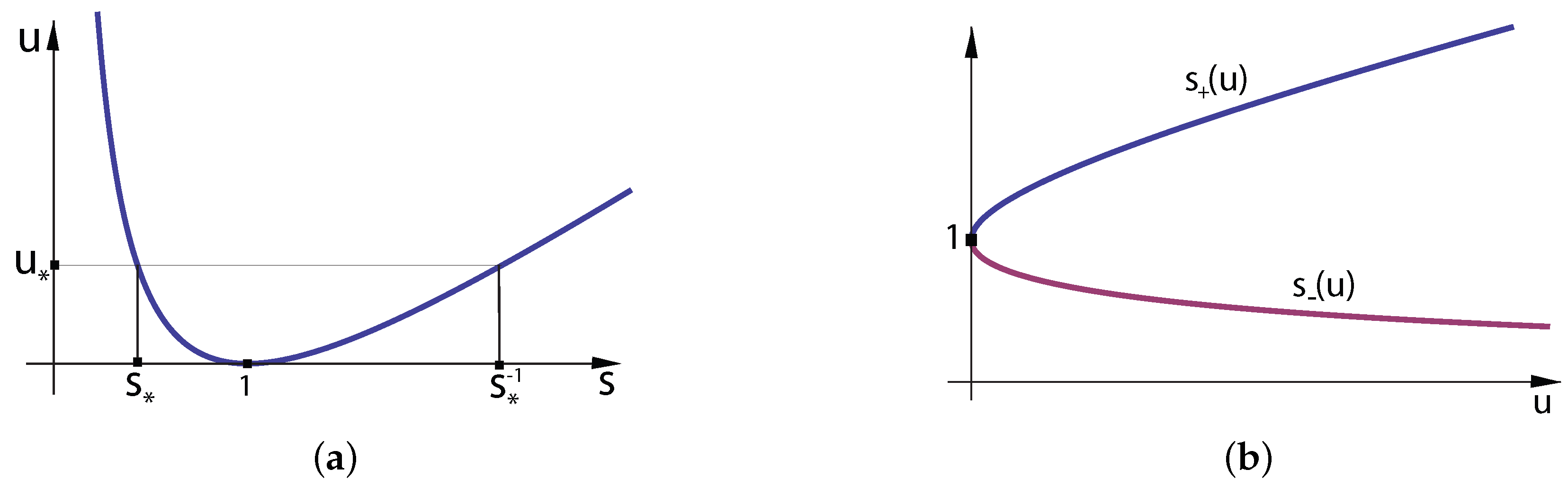
- Second change of variable. The change of variable defined by means of the formula is considered (see Figure 1a), which has two inverse functions,The functions are depicted in Figure 1b. Observe that . The minimum value of is attained at and its value is .This second change of variable determines different integration regions in the new variable u depending on the value of the upper integration limit in (3),When , the integration variable u in (3) runs from to (with , see Figure 1). On the other hand, when , the position of and is interchanged in Figure 1, and then, the integration variable u in (3) runs from to (with ) and also from to (with ). Then, when , only is required in the computation. However, when , then both, and are involved. It is clear from Figure 1 thatwhere
- Third change of variable. The two integrals in the second and third lines of (4) are suitable for an asymptotic analysis when is large by using Watson’s lemma ([14], Chap. 2); a brief and simple version of Watson’s lemma is summarized in Appendix A. This is so because the maximum value of the exponent in the integration interval is attained at , which is the left end point of the integration interval, and only the factor in the denominator of these integrals vanishes at this point, whereas the other factor is analytic there. The situation is different for the integral in the first line of (4). Once again, the maximum value of the exponent in the integration interval is attained at , which is the left end point of the integration interval. However, now, although the whole denominator is analytic there, when the variable t approaches the critical value ( approaches the critical value 1), the integration limit approaches the value zero, where vanishes. Therefore, in the two last integrals, an expansion of the integrand at the asymptotically relevant point is possible for any value of t, and Watson’s lemma can be applied uniformly in the time variable t. On the other hand, in the first integral, this expansion is only possible when the time variable t is bounded away from the critical timeIt is assumed in this discussion that as a function of the variable u, the “composite” pumping functionis analytic at for any value of . This assumption does not mean any restriction from a practical point of view, as any realistic pumping function meets this condition. Nevertheless, the specific requirements for the pumping function will be established below.As an asymptotic expansion of the Moench transform uniformly valid in is sought, the above-mentioned problem needs to be solved. The solution is a third change of variable with . In order to simplify the notation, the following functions are definedand the parameterThen, introducing the change of variable in (4),The asymptotic features of the three integrals have not changed, but now, the factor (in the three integrals) is analytic at the asymptotic relevant point (in the two last integrals) and (in the first one), even when and . However, before proceeding further and apply Watson’s lemma to these integrals, a more compact form of that simplifies computations is considered,where we have introduced the step function and the sign function :
3. Asymptotic Approximation of (7) for a Pumping Function of Power Type
4. Numerical Experiments
5. Conclusions
Author Contributions
Funding
Conflicts of Interest
Appendix A. Watson’s Lemma
Appendix B. Asymptotic Approximation of (7) for a General Pumping Function

References
- Hantush, M.S. Analysis of data from pumping tests in leaky aquifers. Trans. Am. Geophys. Union 1956, 37, 702–714. [Google Scholar] [CrossRef]
- Hantush, M.S. Nonsteady flow to flowing wells in leaky aquifers. J. Geophys. Res. 1959, 64, 1043–1052. [Google Scholar] [CrossRef]
- Hantush, M.S. Modification of the theory of leaky aquifers. J. Geophys. Res. 1960, 65, 3713–3725. [Google Scholar] [CrossRef]
- Hantush, M.S.; Jacob, C.E. Non-steady radial flow in an infinit leaky aquifer. Trans. Am. Geophys. Union 1955, 36, 95–100. [Google Scholar] [CrossRef]
- Lohman, S.W. Ground-Water Hidraulics; U.S. Department of the Interior: Washington, DC, USA, 1972.
- Moench, A. Ground-water fluctuations in response to arbitrary pumping. Groundwater 1971, 9, 4–8. [Google Scholar] [CrossRef]
- Stallman, R.W. Variable discharge without vertical leakage. In Theory of Aquifer Tests; Ferris, J.G., Ed.; U. S. Geological Survey Water-Supply Paper 1536-E; US Government Printing Office: Washington, DC, USA, 1962; pp. 118–122. [Google Scholar]
- Theis, C.V. The relation between lowering of the piezometric surface and the rate and duration of discharge of a well using ground-water storage. Trans. Am. Geophys. Union 1935, 2, 519–524. [Google Scholar] [CrossRef]
- Walton, W.C. Selected Analytical Methods for Well and Aquifer Evaluation; Bulletin (Illinois State Water Survey) No. 49; Department of Registration and Education, State Water Survey Division, State of Illinois: Springfield, IL, USA, 1962.
- Hantush, M.S. Drawdown around a partially penetrating well. J. Hyd. Div. Proc. Am. Soc. Civil Eng. 1961, 87, 83–98. [Google Scholar] [CrossRef]
- Hantush, M.S. Aquifer tests on partially penetrating wels. J. Hyd. Div. Proc. Am. Soc. Civil Eng. 1961, 87, 171–194. [Google Scholar]
- Vandenberg, A. Tables and Type Curves for Analysis of Pump Tests in Leaky Parallel-Channel Aquifers; Technical Bulletin No. 96; Inland Waters Directorate, Water Resources Brach: Ottawa, ON, USA, 1976; 28p.
- Vandenberg, A. Type curves for analysis of pump tests in leaky strip aquifers. J. Hydrol. 1977, 33, 15–26. [Google Scholar] [CrossRef]
- Temme, N.M. Asymptotic Methods for Integrals; World Scientific: Singapore, 2015. [Google Scholar]
- Krätzel, E. Integral transformations of Bessel type. In Generalized Functions and Operational Calculus (Proc. Conf., Varna, 1975); Bulgar. Acad. Sci.: Sofia, Bulgaria, 1979. [Google Scholar]
- Harris, F.E. On Kryachko’s formula for the leaky aquifer function. Int. J. Quantum Chem. 2001, 81, 332–334. [Google Scholar] [CrossRef]
- Kryachko, E.S. Explicit expression for the leaky aquifer function. Int. J. Quantum Chem. 2000, 78, 303–305. [Google Scholar] [CrossRef]
- Harris, F.E. New approach to calculation of the leaky aquifer function. Int. J. Quantum Chem. 1997, 63, 913–916. [Google Scholar] [CrossRef]
- Harris, F.E. More about the leaky aquifer function. Int. J. Quantum Chem. 1998, 70, 623–626. [Google Scholar] [CrossRef]
- Chaudhry, M.A.; Temme, N.M.; Veling, E.J.M. Asymptotics and closed form of a generalized incomplete gamma function. J. Comput. Appl. Math. 1996, 67, 371–379. [Google Scholar]
- Harris, F.E. Incomplete Bessel, generalized incomplete gamma, or leaky aquifer function. J. Comput. Appl. Math. 2008, 215, 260–269. [Google Scholar] [CrossRef]
- Askey, R.A.; Roy, R. Gamma Function. In NIST Handbook of Mathematical Functions; Cambridge University Press: Cambridge, UK, 2010; Chapter 5; pp. 135–147. [Google Scholar]
- Temme, N.M. Error Functions, Dawson’s and Fresnel Integrals. In NIST Handbook of Mathematical Functions; Cambridge University Press: Cambridge, UK, 2010; Chapter 7; pp. 160–170. [Google Scholar]
- Di Bruno, F.F. Theorie des Formes Binaires; Librarie Brero: Torino, Italy, 1876. [Google Scholar]


| n | ||||
|---|---|---|---|---|
| 0 | 6.37 × 10 | 2.75 × 10 | 2.70 × 10 | 2.70 × 10 |
| 2 | 6.26 × 10 | 3.34 × 10 | 3.30 × 10 | 3.30 × 10 |
| 4 | 6.92 × 10 | 7.54 × 10 | 7.43 × 10 | 7.43 × 10 |
| 6 | 8.11 × 10 | 2.50 × 10 | 2.47 × 10 | 2.46 × 10 |
| n | ||||
|---|---|---|---|---|
| 0 | 0.25 | 5.62 × 10 | 4.59 × 10 | 5.93 × 10 |
| 2 | 1.62 × 10 | 3.04 × 10 | 4.59 × 10 | 5.93 × 10 |
| 4 | 1.60 × 10 | 4.93 × 10 | 4.59 × 10 | 5.93 × 10 |
| 6 | 1.78 × 10 | 1.33 × 10 | 4.59 × 10 | 5.93 × 10 |
| n | ||||
|---|---|---|---|---|
| 0 | 0.52 | 6.33 × 10 | 6.30 × 10 | 5.87 × 10 |
| 2 | 3.30 × 10 | 3.42 × 10 | 6.30 × 10 | 5.87 × 10 |
| 4 | 3.26 × 10 | 5.56 × 10 | 6.30 × 10 | 5.87 × 10 |
| 6 | 3.61 × 10 | 1.50 × 10 | 6.30 × 10 | 5.87 × 10 |
| n | ||||
|---|---|---|---|---|
| 0 | 0.16 | 1.77 × 10 | 2.54 × 10 | 2.54 × 10 |
| 2 | 1.46 × 10 | 1.39 × 10 | 3.07 × 10 | 3.07 × 10 |
| 4 | 1.57 × 10 | 2.56 × 10 | 6.90 × 10 | 6.90 × 10 |
| 6 | 1.81 × 10 | 7.50 × 10 | 2.28 × 10 | 2.28 × 10 |
Disclaimer/Publisher’s Note: The statements, opinions and data contained in all publications are solely those of the individual author(s) and contributor(s) and not of MDPI and/or the editor(s). MDPI and/or the editor(s) disclaim responsibility for any injury to people or property resulting from any ideas, methods, instructions or products referred to in the content. |
© 2023 by the authors. Licensee MDPI, Basel, Switzerland. This article is an open access article distributed under the terms and conditions of the Creative Commons Attribution (CC BY) license (https://creativecommons.org/licenses/by/4.0/).
Share and Cite
López, J.L.; Pagola, P.; Pérez Sinusía, E. Asymptotic Expansions for Moench’s Integral Transform of Hydrology. Mathematics 2023, 11, 3053. https://doi.org/10.3390/math11143053
López JL, Pagola P, Pérez Sinusía E. Asymptotic Expansions for Moench’s Integral Transform of Hydrology. Mathematics. 2023; 11(14):3053. https://doi.org/10.3390/math11143053
Chicago/Turabian StyleLópez, José L., Pedro Pagola, and Ester Pérez Sinusía. 2023. "Asymptotic Expansions for Moench’s Integral Transform of Hydrology" Mathematics 11, no. 14: 3053. https://doi.org/10.3390/math11143053
APA StyleLópez, J. L., Pagola, P., & Pérez Sinusía, E. (2023). Asymptotic Expansions for Moench’s Integral Transform of Hydrology. Mathematics, 11(14), 3053. https://doi.org/10.3390/math11143053