Stochastic Comparisons of Lifetimes of Used Standby Systems

Abstract

In this paper, we first establish upper stochastic bounds on the lifetime of a used cold standby system with arbitrary age, using the likelihood ratio order and the usual stochastic order. Then, stochastic comparisons are made between the lifetime of a used cold standby system with age t and the lifetime of a cold standby system consisting of used components with age t using the likelihood ratio order and the usual stochastic order. We use illustrative examples to explore the results presented.

1. Introduction and Preliminaries

Cold standby systems are backup systems that are not ready for use until they are needed. In other words, they are kept on standby but are not actively operated. This type of backup system is commonly used in situations where the primary system has a long lifetime and is unlikely to fail frequently (see, e.g., Kumar and Agarwal [1], Kou and Zuo [2], Yang [3], and Peng et al. [4]). Reliability analysis of cold standby systems involves evaluating the probability of failure of the primary system and the time required to switch to the backup system. The reliability of the primary system is determined by analyzing its failure rate, while the reliability of the backup system is determined by analyzing its startup time and the probability of failure during startup. In the context of replacement strategies and related optimization problems, cold standby systems have been used repeatedly in the literature (see, e.g., Coit [5], Yu et al. [6], Jia and Wu [7], Xing et al. [8], and Ram et al. [9]).

Several methods can be used to analyze the reliability of cold standby systems, including fault tree analysis, reliability block diagrams, and Markov models. These methods allow engineers to identify potential failure modes, estimate the probability of system failure, and evaluate the effectiveness of backup systems. The study of the reliability of complex systems using cold standby systems has been conducted by many researchers for engineering problems (see, for example, Azaron et al. [10], Wang et al. [11], Wang et al. [12], and Behboudi et al. [13]).

Stochastic comparisons between the random lifetimes of various complex systems have been a subject of increasing interest among engineers and system designers. This enables them to have, for example, an optimization problem to solve and, consequently, a plan to prepare a product with greater reliability. The theory of stochastic orderings in applied probability has been recently utilized to compare the lifetime of coherent systems equipped with cold standby units from a stochastic point of view (cf. Boland and El-Neweihi [14], Li et al. [15], Eryilmaz [16], Eryilmaz [17], Roy and Gupta [18] and Roy and Gupta [19]). The study of stochastic orders between lifetime of a used coherent system and lifetime of a coherent system with used components has attracted the attention of many researchers (see, e.g., Gupta [20], Li et al. [21], and Hazra and Nanda [22], among others). To highlight the novelty of our contribution in the continuing part, it is mentioned here that a cold standby system cannot be considered as a particular coherent system.

The problem of stochastic orders among lifetime of a used cold standby system and lifetime of another cold standby system composed of used components has not been studied in the literature. Stochastic comparisons of lifetimes of general cold standby systems with an arbitrary age have also not been considered in the literature thus far. As will be clarified in the sequel, the lifetime of a cold standby system comprising one component with additional $(n-1)$ cold standby spares is the sum of random variables; thus, in this regard, a few studies may be found in Zhao and Balakrishnan [23], Amiri et al. [24], Khaledi and Amiri [25], and Amiripour et al. [26], among others.

In the current study, we develop some stochastic ordering results using the well-known usual stochastic order and the likelihood ratio order, involving the lifetime of a used cold standby system with an arbitrary age, and provide some bounds for the reliability function (rf) of the lifetime of such a system. The usual stochastic ordering is associated with ordering two systems according to their reliability functions, which is quite relevant in this context. Likelihood ratio ordering is also a powerful tool for ordering systems according to their reliability functions, after making a certain statement about the lifetimes of the systems in a given interval. Consider a situation where the interval $(t,\tau ]$ is considered the time of use for a standby system. For example, in practice, there are situations where a product (a standby system or its components) undergoes a burn-in process immediately after manufacturing. Therefore, t can be the burn-in time of the product and $\tau$ can be the time at which a system is placed out of service. We then use the likelihood ratio order (which is a strong stochastic order) to compare the reliability of two systems in their times of use. The rf of the lifetime of a cold standby system with used components of the age t is used to provide upper bound and lower bound for the rf of the used cold standby system with age t.

In the sequel we will use some notations. Let $\mathrm{X}̠=(X_1,\dots ,X_n)$ be a random vector and $\mathrm{x}̠=(x_1,\dots ,x_n)$ be a vector of observations as a realization of $\mathrm{X}̠$. Denote $S_{m,\mathrm{X}̠}={\sum }_{i=1}^m{X}_i$ and $S_{m,\mathrm{x}̠}={\sum }_{i=1}^m{x}_i$ with $m=1,2,\dots ,n$. Consider the cold standby system consisting of n components. Initially, one component starts working and the other $n-1$ components are in cold standby mode. When the working component fails, the components in standby mode are replaced one by one until all components have failed and the cold standby system fails. The cold standby system means that the components do not fail or degrade in standby mode and that the standby period does not affect the life of the components in future use. When the failed component is replaced by the standby component, the switch is absolutely reliable and transmission is instantaneous. Let $X_1,\dots ,X_n$ be the lifetimes of the n components with cumulative distribution functions $F_{X_1},\dots ,F_{X_n}$ and corresponding rfs ${\stackrel{-}{F}}_{X_1},\dots ,{\stackrel{-}{F}}_{X_n}$. We also assume that $X_1,\dots ,X_n$ are independent. Then, the lifetime of the cold standby system is

$$S_{n,\mathrm{X}̠}=X_1+X_2+\dots +X_n.$$

(1)

The rf of the lifetime of the cold standby system given in (1) is

$${\stackrel{-}{F}}_{S_{n,\mathrm{X}̠}}\left(t\right)=P(X_1+X_2+\dots +X_n>t)={\stackrel{-}{F}}_{X_1}\left(t\right)\ast {\stackrel{-}{F}}_{X_2}\left(t\right)\ast \dots \ast {\stackrel{-}{F}}_{X_n}\left(t\right),$$

(2)

where ∗ represents the convolution operator. It is known that when $X_i$ and $X_j$ for $i\ne j$ are independent, then ${\stackrel{-}{F}}_{X_i}\left(t\right)\ast {\stackrel{-}{F}}_{X_j}\left(t\right)={\int }_{-\infty }^{+\infty }{\stackrel{-}{F}}_{X_i}(t-x)f_{X_j}\left(x\right)dx,$ where $f_{X_j}$ is the probability density function (pdf) of $X_j$, which is the rf of the convolution of $X_i$ and $X_j$, i.e., the rf of $X_i+X_j$. Thus, from (2), we can write

$${\stackrel{-}{F}}_{S_{n,\mathrm{X}̠}}\left(t\right)={\stackrel{-}{F}}_{S_{n-1,\mathrm{X}̠}}\left(t\right)\ast {\stackrel{-}{F}}_{X_n}\left(t\right)={\int }_{-\infty }^{+\infty }{\stackrel{-}{F}}_{S_{n-1,\mathrm{X}̠}}(t-x)f_{X_n}\left(x\right)dx.$$

(3)

We will need some other preliminaries in the continuing part of the paper. Suppose that X is the lifetime of a fresh item as its lifespan. We may need to recognize the distribution of the lifetime of that item at the age t. The random variable (rv) $X_t=[X-t|X>t]$, which is called the residual lifetime of an item with original life length X at the time t provided that the item is already alive at this time, is ordinarily utilized to represent and model the lifetime of a used component or item. Let X have pdf $f_X$ (whenever it exists) and rf ${\stackrel{-}{F}}_X$. Then, $X_t$ has pdf

$$f_{X_t}\left(x\right)=\frac{f_X(t+x)}{{\stackrel{-}{F}}_X\left(t\right)}dx,x\ge 0,$$

and it has rf

$${\stackrel{-}{F}}_{X_t}\left(x\right)=\frac{{\stackrel{-}{F}}_X(t+x)}{{\stackrel{-}{F}}_X\left(t\right)}:x\ge 0,$$

which are valid as $t\in \{t\ge 0:{\stackrel{-}{F}}_X\left(t\right)>0\}.$ The mean residual lifetime (MRL) function of X is given by

$$m_X\left(t\right)=E[X-t|X>t]={\int }_t^{+\infty }\frac{{\stackrel{-}{F}}_X\left(x\right)}{{\stackrel{-}{F}}_X\left(t\right)}dx,t\in \{t\ge 0:{\stackrel{-}{F}}_X\left(t\right)>0\}.$$

Stochastic ordering of distributions has been a useful tool for statisticians in the context of testing statistical hypothesises. Two well-known stochastic orders will be used throughout this paper. The following definition can be found in Shaked and Shanthikumar [27].

Definition 1.

Let X and Y be two non-negative rvs with pdfs $f_X$ and $f_Y$, and rfs ${\stackrel{-}{F}}_X$ and ${\stackrel{-}{F}}_Y$, respectively. Then, it is said that X is smaller or equal than Y in the

(i)

Likelihood ratio order (denoted by $X{\le }_{lr}Y$) whenever $\frac{f_Y\left(t\right)}{f_X\left(t\right)}$ is nondecreasing in $t\ge 0$.

(ii)

Usual stochastic order (denoted by $X{\le }_{st}Y$) whenever ${\stackrel{-}{F}}_X\left(t\right)\le {\stackrel{-}{F}}_Y\left(t\right),$ for all $t\ge 0$.

The stochastic orders in Definition 1 are connected to each other, as it has been proven that $X{\le }_{lr}Y$ implies $X{\le }_{st}Y$ (see, e.g., Shaked and Shanthikumar [27]). Nonparametric classes of life distributions are usually based on the pattern of aging in some sense. For example, by comparing $X_{t_1}$ with $X_{t_2}$ for $t_1\le t_2$ as two time points according to the likelihood ratio order, new patterns of aging are produced. The common parametric families of life distributions also feature monotone aging. In this context, the following definition is also applied in the paper.

Definition 2.

The rv X with pdf $f_X$ is said to have

(i)

Increasing likelihood ratio property (denoted as $X\in ILR$) whenever $f_X\left(t\right)$ is log-concave in $t\ge 0$.

(ii)

Decreasing likelihood ratio property (denoted as $X\in DLR$) whenever $f_X\left(t\right)$ is log-convex in $t\ge 0$.

For example, the exponential distribution has both $ILR$ and $DLR$ properties. The gamma distribution with shape parameter $\alpha$ and scale parameter $\lambda$ has $ILR$ property if $\alpha >1$ and it has $DLR$ property if $\alpha <1$. For recognizing $ILR$ and $DLR$ properties in further well-known distributions we refer the readers to Bagnoli and Bergstrom [28]. The following definition is due to Karlin [29].

Definition 3.

Suppose that $h(x,y)$ is a non-negative function for all $x\in \mathfrak{X}\subseteq \mathbb{R}$ and for all $y\in \mathfrak{Y}\subseteq \mathbb{R}$. Then, it is said that $h(x,y)$ is totally positive of order 2 (denoted as $T{P}_2$) in $(x,y)\in \mathfrak{X}\times \mathfrak{Y}$, whenever $h(x_1,y_1)h(x_2,y_2)\ge h(x_1,y_2)h(x_2,y_1)$ for all $x_1\le x_2\in \mathfrak{X}$ and for all $y_1\le y_2\in \mathfrak{Y}.$

According to Definition 3, by using the convention that $a/0=+\infty$ for any $a>0$, then $h(x,y)$ is $T{P}_2$ in $(x,y)$ in the desired subset of ${\mathbb{R}}^2$, i.e., over the set $\mathfrak{X}\times \mathfrak{Y}$ if, and only if, $\frac{h(x_2,y)}{h(x_1,y)}$ is nondecreasing in $y\in \mathfrak{Y}$, or, equivalently, if $\frac{h(x,y_2)}{h(x,y_1)}$ is nondecreasing in $x\in \mathfrak{X}$.

2. Stochastic Bounds for the Lifetime of a Used Standby System

Let us consider independent and non-negative rvs $X_1,X_2,\dots ,X_n$, and denote by $X_1\left(t\right),X_2\left(t\right),\dots$, $X_n\left(t\right)$ the corresponding conditional rvs, so that $X_i\left(t\right)=\left[X_i\right|X_i>t]$, for all $t\ge 0$ for which $R_{X_i}\left(t\right)>0$. Note that for the random vector $\mathrm{Z}̠=(Z_1,Z_2,\dots ,Z_m)$, the conditional rv $[\mathrm{Z}̠|\mathrm{Z}̠\in A]$ is a vector-valued rv whose joint distribution is equal with conditional join distribution of $\mathrm{Z}̠$ give $\mathrm{Z}̠\in A$, where A is a subset of ${\mathbb{R}}^m$ for which $P(\mathrm{Z}̠\in A)>0$. The rv $X_i\left(t\right)$ has pdf

$$f_{X_i\left(t\right)}\left(x\right)=\frac{f_{X_i}\left(x\right)I[x>t]}{R_{X_i}\left(t\right)}.$$

(4)

Consider, now, the vector $\mathrm{X}̠\left(t\right)=(X_1,X_2,\dots ,X_n|X_1>t,X_2>t,\dots ,X_n>t)$ which, since $X_i$s are independent, it has joint cdf

$$f_{\mathrm{X}̠\left(t\right)}(\mathrm{x}̠)=\prod _{i=1}^n\frac{f_{X_i}\left(x_i\right)I[x_i>t]}{R_{X_i}\left(t\right)},$$

(5)

where $I[x_i>t]$ is the indicator function of the set $[x_i>t]$, i.e., $I[x_i>t]=0,$ when $x_i\le t$ and $I[x_i>t]=1$ if $x_i>t$. Note that the ith marginal distribution of $\mathrm{X}̠\left(t\right)$ is the distribution of $X_i\left(t\right)$ provided that $X_1,X_2,\dots ,X_n$ are independent. We can find that for any function $\psi :{\mathbb{R}}^n\mapsto \mathbb{R}$,

$$E\left[\psi (\mathrm{X}̠\left(t\right))\right]=\frac{E\left[\psi \right(\mathrm{X}̠\left)I\right[\mathrm{x}̠>\mathrm{t}̠\left]\right]}{{\stackrel{-}{F}}_{X̠}(\mathrm{t}̠)}$$

(6)

where $\mathrm{t}̠=(t,t,\dots ,t)$ is a vector with size n and ${\stackrel{-}{F}}_{X̠}$ is the joint reliability function of $\mathrm{X}̠$. We will utilize $\psi (\mathrm{x}̠)=S_{n,\mathrm{x}̠}.$ Note that $\left(S_{n,\mathrm{X}̠}\right)\left(t\right)$ is equal in distribution with the conditional rv $\left[S_{n,\mathrm{X}̠}\right|S_{n,\mathrm{X}̠}>t]$, where $S_{n,\mathrm{X}̠}={\sum }_{i=1}^n{X}_i$. The following lemma will be used in the sequel.

Lemma 1.

Let $X̠=(X_1,X_2,\dots ,X_n)$ be a random vector, having joint pdf $f_{X̠}(x̠)$. Consider $Y̠=(Y_1,Y_2,\dots ,Y_n)$ as a random vector with joint pdf

$$f_{Y̠}(\underset{¯}{y})=\frac{I[S_{n,\underset{¯}{y}}>t]f_{X̠}(\underset{¯}{y})}{P(S_{n,X̠}>t)}.$$

(7)

Then, $\left(S_{n,X̠}\right)\left(t\right){=}_{st}{S}_{n,Y̠}$, where ${=}_{st}$ means equality in distribution.

Proof. 

It is sufficient to show that $R_{\left(S_{n,\mathrm{X}̠}\right)\left(t\right)}\left(s\right)=R_{S_{n,\mathrm{Y}̠}}\left(s\right),$ for all $s\ge 0$. We can write

$$\begin{array}{cc}\hfill R_{\left(S_{n,\mathrm{X}̠}\right)\left(t\right)}\left(s\right)& =P(\left(S_{n,\mathrm{X}̠}\right)\left(t\right)>s)\hfill \\ \hfill & =P(S_{n,\mathrm{X}̠}>s|S_{n,\mathrm{X}̠}>t)\hfill \\ \hfill & =\left\{\begin{array}{cc}1\hfill & \hfill :s\le t\\ \hfill & \hfill \\ \frac{R_{S_{n,\mathrm{X}̠}}\left(s\right)}{R_{S_{n,\mathrm{X}̠}}\left(t\right)}\hfill & \hfill :s>t.\end{array}\right.\hfill \end{array}$$

On the other hand, from (24), we obtain

$$\begin{array}{cc}\hfill R_{S_{n,\mathrm{Y}̠}}\left(s\right)& =P(S_{n,\mathrm{Y}̠}>s)\hfill \\ \hfill & =\frac{P(S_{n,\mathrm{X}̠}>t\vee s)}{P(S_{n,\mathrm{X}̠}>t)}\hfill \\ \hfill & =\left\{\begin{array}{cc}1\hfill & \hfill :s\le t\\ \hfill & \hfill \\ \frac{R_{S_{n,\mathrm{X}̠}}\left(s\right)}{R_{S_{n,\mathrm{X}̠}}\left(t\right)}\hfill & \hfill :s>t,\end{array}\right.\hfill \end{array}$$

in which $t\vee s=max\{t,s\}$. Thus, we proved the desired identity and, hence, the result follows. □

The following result indicates that the lifetime of a used standby system of age t with n components is dominated in the sense of the usual stochastic order by the lifetime of a standby system composed of used components plus $(n-1)t$. Denote by $X_{i,t}=[X_i-t|X_i>t]$ which is valid for all $t\ge 0$ for which $R_{X_i}\left(t\right)>0$ and note that $X_i$ is the random lifetime of the ith component in the standby system, with $i=1,2,\dots ,n$. Denote

$$\mathrm{X}{̠}_t=(X_1-t,X_2-t,\dots ,X_n-t|X_1>t,X_2>t,\dots ,X_n>t),t:P(\mathrm{X}̠>tI)>0,$$

where $I={(1,1,\dots ,1)}^{\top }$ is a vector with n components and $\mathrm{X}̠={(X_1,X_2,\dots ,X_n)}^{\top }$. Notice that the marginal distribution of the ith random element in ${\mathrm{X}̠}_t$ corresponds with the distribution of $X_{i,t}$, $i=1,2,\dots ,n$, provided that $X_1,X_2,\dots ,X_n$ are independent.

Theorem 1.

Let $X_1,X_2,\dots ,X_n$ be independent rvs which are non-negative and $X_{1,t},X_{2,t},\dots ,X_{n,t}$ be also independent, for a fixed $t>0$. Then:

$${\left(S_{n,X̠}\right)}_t{\le }_{st}{S}_{n,X{̠}_t}+(n-1)t.$$

(8)

Proof. 

For $n=1$, the result is trivial. Let us assume that $n=2$. From Lemma 1, we can find rvs $Y_1$ and $Y_2$ with joint pdf

$$f_{\mathrm{Y}̠}(\underset{¯}{\mathrm{y}})=\frac{I[S_{2,\underset{¯}{\mathrm{y}}}>t]f_{\mathrm{X}̠}(\underset{¯}{\mathrm{y}})}{R_{S_{2,\mathrm{x}̠}}\left(t\right)},y_i\ge 0,i=1,2,$$

(9)

in which $\underset{¯}{\mathrm{y}}=(y_1,y_2),$ such that $\left(S_{2,\mathrm{X}̠}\right)\left(t\right){=}_{st}{S}_{2,\mathrm{Y}̠}$. From (9), since $X_1$ and $X_2$ are independent, $Y_1$ has pdf

$$f_{Y_1}\left(y_1\right)=\frac{f_{X_1}\left(y_1\right)R_{X_2}(t-y_1)}{R_{S_{2,\mathrm{x}̠}}\left(t\right)}.$$

Then:

$$\begin{array}{cc}\hfill \frac{f_{Y_1}\left(y_1\right)}{f_{X_1\left(t\right)}\left(y_1\right)}& =\frac{R_{X_1}\left(t\right)R_{X_2}(t-y_1)}{R_{S_{2,\mathrm{x}̠}}\left(t\right)I[y_1>t]}\hfill \\ \hfill & =\left\{\begin{array}{cc}+\infty \hfill & \hfill :y_1\le t\\ \hfill & \hfill \\ \frac{R_{X_1}\left(t\right)}{R_{S_{2,\mathrm{X}̠}}\left(t\right)}\hfill & \hfill :y_1>t.\end{array}\right.\hfill \end{array}$$

It is clear that $\frac{f_{Y_1}\left(y_1\right)}{f_{X_1\left(t\right)}\left(y_1\right)}$ is decreasing in $y_1$; thus, $Y_1{\le }_{lr}{X}_1\left(t\right).$ Since ${\le }_{lr}$ implies ${\le }_{st}$,

$$Y_1{\le }_{st}{X}_1\left(t\right).$$

(10)

By Equation (9), the conditional pdf of $Y_2$ given $Y_1=y_1$ is derived as follows:

$$f_{Y_2|Y_1}\left(y_2\right|y_1)=\frac{f_{X_2}\left(y_2\right)I[S_{2,y̠}>t]}{R_{X_2}(t-y_1)}.$$

For any $y_1\ge 0,$ we show that $\frac{f_{Y_2|Y_1}\left(y_2\right|y_1)}{f_{X_2\left(t\right)}\left(y_2\right)}$ is decreasing in $y_2\ge 0$, as $y_1+y_2>t$. We have

$$\frac{f_{Y_2|Y_1}\left(y_2\right|y_1)}{f_{X_2\left(t\right)}\left(y_2\right)}=\left\{\begin{array}{cc}+\infty \hfill & \hfill :y_2\le t,y_1>t-y_2\\ \hfill & \hfill \\ \frac{R_{X_2}\left(t\right)}{R_{X_2}(t-y_1)}\hfill & \hfill :y_2>t,y_1>t-y_2,\end{array}\right.$$

which is decreasing in $y_2\ge 0.$ Therefore, $\left[Y_2\right|Y_1=y_1]{\le }_{lr}{X}_2\left(t\right)$. Hence,

$$\left[Y_2\right|Y_1=y_1]{\le }_{st}{X}_2\left(t\right).$$

(11)

From Equations (10) and (11), using Theorem 6.B.3 in Shaked and Shanthikumar [27], one obtains

$$[X_1+X_2|X_1+X_2>t]=\left(S_{2,\mathrm{X}̠}\right)\left(t\right){\le }_{st}{X}_1\left(t\right)+X_2\left(t\right).$$

It is easily verified that $\left(S_{2,\mathrm{X}̠}\right)\left(t\right){\le }_{st}{S}_{2,\mathrm{X}̠\left(t\right)},$ holds if, and only if, $\left(S_{2,\mathrm{X}̠}\right)\left(t\right)-t{\le }_{st}{S}_{2,\mathrm{X}̠\left(t\right)}-t$. Thus, ${\left(S_{2,\mathrm{X}̠}\right)}_t{\le }_{st}{S}_{2,{\mathrm{X}̠}_t}+t,$ i.e., (13) holds when $n=2$. Finally, we prove the result by induction. Suppose that for $n=m\ge 2,$ it holds that ${\left(S_{m,\mathrm{X}̠}\right)}_t{\le }_{st}{S}_{m,{\mathrm{X}̠}_t}+(m-1)t$. From preservation property of ${\le }_{st}$ under a change in location of distributions, we have

$$S_{m,\mathrm{X}̠}\left(t\right){\le }_{st}{S}_{m,\mathrm{X}̠\left(t\right)}.$$

(12)

From (12), since for $m=2$ the result was proved, an application of Theorem 1.A.3(b) in Shaked and Shanthikumar [27] yields:

$$\begin{array}{cc}\hfill S_{m+1,\mathrm{X}̠}\left(t\right)& {\le }_{st}{S}_{m,\mathrm{X}̠}\left(t\right)+X_{m+1}\left(t\right)\hfill \\ \hfill & {\le }_{st}{S}_{m,\mathrm{X}̠\left(t\right)}+X_{m+1}\left(t\right)\hfill \\ \hfill & {=}_{st}{S}_{m+1,\mathrm{X}̠\left(t\right)}.\hfill \end{array}$$

Equivalently, one can write ${\left(S_{m+1,\mathrm{X}̠}\right)}_t{\le }_{st}{S}_{m+1,{\mathrm{X}̠}_t}+mt$. Hence, the proof is obtained. □

In the context of Theorem 1, one may realize that, if in (13), $t=0$, then ${\le }_{st}$ becomes ${=}_{st}$. Using Theorem 1, an upper bound for the mean residual lifetime (MRL) function of a standby system can be provided. Since ${\le }_{st}$ implies the expectation order, thus, from Theorem 1,

$$\begin{array}{cc}\hfill m_{S_{n,\mathrm{X}̠}}\left(t\right)& =E\left[{\left(S_{n,\mathrm{X}̠}\right)}_t\right]\hfill \\ \hfill & \le E\left[S_{n,\mathrm{X}{̠}_t}\right]+(n-1)t\hfill \\ \hfill & =\sum _{i=1}^n{m}_{X_i}\left(t\right)+(n-1)t,\hfill \end{array}$$

where $m_{S_{n,\mathrm{X}̠}}\left(t\right)=E[{\sum }_{i=1}^n{X}_i-t|{\sum }_{i=1}^n{X}_i>t]$ is the MRL function of a standby system with independent component lifetimes $X_1,X_2,\dots ,X_n$, and $m_{X_i}\left(t\right)=E\left[X_{i,t}\right]$ is the MRL function of $X_i$ for $i=1,2,\dots ,n$. The bound provided for the MRL function of a standby system is valuable because the MRL function of the system which depends on the distribution of convolution of n rvs, which has no closed form in many situation, does not have an explicit formula. The rv X has a gamma distribution with the shape parameter $\alpha$ and the scale parameter $\lambda$ whenever X has density $f_X\left(x\right)=\frac{{\lambda }^{\alpha }{x}^{\alpha -1}{e}^{-\lambda x}}{\mathsf{\Gamma }\left(\alpha \right)}$ (denote it by $X_i\sim G(\alpha ,\lambda )$). Let us suppose that under consideration is a standby system with independent heterogeneous exponential component lifetimes $X_1,X_2,\dots ,X_n$, so that $X_i$ has mean $\frac{1}{{\lambda }_i}$ ($X_i\sim Exp\left({\lambda }_i\right)$), where ${\lambda }_i>0,i=1,2,\dots ,n$. It is known that $m_{X_i}\left(t\right)=\frac{1}{{\lambda }_i}$; however, the $S_{n,\mathrm{X}̠}={\sum }_{i=1}^n{X}_i$ as the random lifetime of the standby system has a gamma distribution ($S_{n,\mathrm{X}̠}\sim G(n,{\sum }_{i=1}^n{\lambda }_i)$) with an indefinite MRL function. However,

$$m_{S_{n,\mathrm{X}̠}}\left(t\right)\le \sum _{i=1}^n\frac{n}{{\lambda }_i}+(n-1)t,\mathrm{for}\mathrm{all}t\ge 0.$$

In the following example, the result of Theorem 1 is applied.

Example 1.

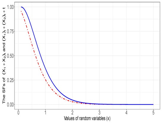
Suppose that $X_1\sim G(2,3)$ and $X_2\sim G(1/2,3)$ are two independent rvs and assume that $X_{1,t}$ and $X_{2,t}$ are also independent. Note that $X_1\in ILR$ and $X_2\in DLR$. Consider a two-units standby system. Using Theorem 1, an upper bound for the rf of the used standby system with age $t=0.1$ is derived. Specifically, it is shown that

$${\left(S_{2,X̠}\right)}_t={(X_1+X_2)}_t{\le }_{st}{X}_{1,t}+X_{2,t}+t=S_{2,X{̠}_t}+t.$$

Since it is trivial that for all $x\le 0.1,$ one has $P(S_{2,X{̠}_t}+t>x)=1$; thus, for all $x\le 0.1$, $P(S_{2,X{̠}_t}+t>x)\ge P({\left(S_{2,X̠}\right)}_t>x)$. Therefore, it is enough to show that $P(S_{2,X{̠}_t}+t>x)\ge P({\left(S_{2,X̠}\right)}_t>x),$ for all $x>0.1$. It is seen that for $t=0.1$

$$P({\left(S_{2,X̠}\right)}_t>x)=\frac{{\stackrel{-}{F}}_{X_1+X_2}(0.1+x)}{{\stackrel{-}{F}}_{X_1+X_2}\left(0.1\right)}=\frac{{\int }_{0.1+x}^{+\infty }{u}^{\frac{3}{2}}exp(-3u)du}{{\int }_{0.1}^{+\infty }{u}^{\frac{3}{2}}exp(-3u)du}.$$

On the other hand, for all $x>0.1$, we can obtain

$$P(S_{2,X{̠}_t}+t>x)={\int }_{0.1}^x{\stackrel{-}{F}}_{X_{1,0.1}}(x-x_2)f_{X_{2,0.1}}(x_2-0.1)d{x}_2+{\stackrel{-}{F}}_{X_{2,0.1}}(x-0.1),$$

in which the rf of $X_{1,0.1}=[X_1-0.1|X_1>0.1]$ is acquired as

$${\stackrel{-}{F}}_{X_{1,0.1}}\left(x\right)=\frac{{\stackrel{-}{F}}_{X_1}(0.1+x)}{{\stackrel{-}{F}}_{X_1}\left(0.1\right)}=\frac{(1+3(0.1+x\left)\right)exp(-3(0.1+x\left)\right)}{1.3exp(-0.3)},$$

and, similarly, the rf of $X_{2,0.1}=[X_2-0.1|X_2>0.1]$ is obtained as

$${\stackrel{-}{F}}_{X_{2,0.1}}\left(x\right)=\frac{{\stackrel{-}{F}}_{X_2}(0.1+x)}{{\stackrel{-}{F}}_{X_2}\left(0.1\right)}=\frac{{\int }_{0.1+x}^{+\infty }{u}^{-\frac{1}{2}}exp(-3u)du}{{\int }_{0.1}^{+\infty }{u}^{-\frac{1}{2}}exp(-3u)du},$$

and, consequently,

$$f_{X_{2,0.1}}\left(x\right)=\frac{{(0.1+x)}^{-\frac{1}{2}}exp(-3(x+0.1))}{{\int }_{0.1}^{+\infty }{u}^{-\frac{1}{2}}exp(-3u)du}.$$

In Figure 1, the graph of SFs of ${\left(S_{2,X̠}\right)}_t$ and $S_{2,X{̠}_t}+t$ is plotted, which makes it clear that for $0.1<x<5$, $P(S_{2,X{̠}_t}+t>x)\ge P{\left(S_{2,X̠}\right)}_t)$ when $t=0.1$.

Figure 1. Plot of the rf of $S_{2,\mathrm{X}{̠}_t}+t$ (solid line) and the rf of ${\left(S_{2,\mathrm{X}̠}\right)}_t$ (dot-dashed line) for $t=0.1$ and for $x\in (0.1,5)$.

In the sequel of this section, the result of Theorem 1 is strengthened to the case where the likelihood ratio order is used. However, in this case, the random lifetimes of the components need to to have log-concave density functions, which means that the components lifetimes have to fulfill the ILR property. We first give the following technical lemmas. The proof of the following lemmas, being straightforward, are omitted.

Lemma 2.

Suppose that Y and Z are two rvs with pdfs $f_Y$ and $f_Z,$ respectively. The following assertions hold:

(a)

If Y has support $S_Y=(l_Y,+\infty )$ and Z has support $S_Z=(l_Z,+\infty ),$ so that $l_Y\ge l_Z$, then $Y{\ge }_{lr}Z$ if, and only if, $\frac{f_Y\left(s\right)}{f_Z\left(s\right)}$ is nondecreasing in $s>l_Y$.

(b)

If $Y{\ge }_{lr}Z$, then $Y-c{\ge }_{lr}Z-c,$ for $c>0$.

Lemma 3.

The following assertions hold true:

(a)

For any non-negative rv W, for all $t\ge 0$ for which $P(W>t)>0$, it holds that $W_t{=}_{st}W\left(t\right)-t$ where $W_t=[W-t|W>t]$ and $W\left(t\right)=\left[W\right|W>t].$

(b)

For all $t\ge 0,$ for which $P(X_i>t)>0,i=1,2,\dots ,n$ it holds that $S_{n,X̠\left(t\right)}{=}_{st}{S}_{n,X{̠}_t}+nt$.

Theorem 2.

Let $X_1,X_2,\dots ,X_n$ be non-negative independent rvs which are all $ILR$, and suppose that $X_{1,t},X_{2,t},\dots ,X_{n,t}$ are independent, for a fixed $t>0$. Then:

$${\left(S_{n,X̠}\right)}_t{\le }_{lr}{S}_{n,X{̠}_t}+(n-1)t.$$

(13)

Proof. 

Fix $t>0$. Firstly, we prove that

$$Y=S_{n,\mathrm{X}̠\left(t\right)}{\ge }_{lr}\left(S_{n,\mathrm{X}̠}\right)\left(t\right)=Z,$$

in which $S_{n,\mathrm{X}̠\left(t\right)}={\sum }_{i=1}^n{X}_i\left(t\right)$ and $\left(S_{n,\mathrm{X}̠}\right)\left(t\right)=\left({\sum }_{i=1}^n{X}_i\right)\left(t\right)$ with $X_i\left(t\right)=\left[X_i\right|X_i>t]$. Since $l_Y=nt$ and $l_Z=t$, by Lemma 2 it is enough to show that $\frac{f_Y\left(s\right)}{f_Z\left(s\right)}$ is nondecreasing in s for all $s>nt$. One has

$$\begin{array}{cc}\hfill f_Z\left(s\right)& =\frac{f_{S_{n,\mathrm{X}̠}}\left(s\right)I[s>t]}{R_{S_{n,\mathrm{X}̠}}\left(t\right)}\hfill \\ \hfill & =\frac{f_{S_{n,\mathrm{X}̠}}\left(s\right)}{R_{S_{n,\mathrm{X}̠}}\left(t\right)},s>nt.\hfill \end{array}$$

Denote $S_{n-1,\mathrm{X}̠\left(t\right)}={\sum }_{i=1}^{n-1}{X}_i\left(t\right)$, and similarly, $S_{n-1,\mathrm{X}̠}={\sum }_{i=1}^{n-1}{X}_i$. Therefore, for all $s>nt,$ in light of the Equation (3), one can derive

$$\begin{array}{cc}\hfill \frac{f_Y\left(s\right)}{f_Z\left(s\right)}& =R_{S_{n,\mathrm{X}̠}}\left(t\right)\frac{{\int }_0^{+\infty }{f}_{X_n\left(t\right)}(s-y)f_{S_{n-1,\mathrm{X}̠\left(t\right)}}\left(y\right)dy}{{\int }_0^{+\infty }{f}_{X_n}(s-y)f_{S_{n-1,\mathrm{X}̠}}\left(y\right)dy}\hfill \\ \hfill & =\frac{R_{S_{n,\mathrm{X}̠}}\left(t\right)}{R_{X_n}\left(t\right)}\frac{{\int }_0^{s-t}{f}_{X_n}(s-y)f_{S_{n-1,\mathrm{X}̠\left(t\right)}}\left(y\right)dy}{{\int }_0^s{f}_{X_n}(s-y)f_{S_{n-1,\mathrm{X}̠}}\left(y\right)dy}\hfill \\ \hfill & =\frac{R_{S_{n,\mathrm{X}̠}}\left(t\right)}{R_{X_n}\left(t\right)}{\int }_0^s\frac{f_{S_{n-1,\mathrm{X}̠\left(t\right)}}\left(y\right)}{f_{S_{n-1,\mathrm{X}̠}}\left(y\right)}\frac{I[y<s-t]f_{X_n}(s-y)f_{S_{n-1,\mathrm{X}̠}}\left(y\right)}{{\int }_0^s{f}_{X_n}(s-y)f_{S_{n-1,\mathrm{X}̠}}\left(y\right)dy}dy\hfill \\ \hfill & =\frac{R_{S_{n,\mathrm{X}̠}}\left(t\right)}{R_{X_n}\left(t\right)}{\int }_0^s\frac{f_{S_{n-1,\mathrm{X}̠\left(t\right)}}\left(y\right)}{f_{S_{n-1,\mathrm{X}̠}}\left(y\right)}\frac{I[y<s-t]f_{X_n}(s-y)f_{S_{n-1,\mathrm{X}̠}}\left(y\right)}{{\int }_0^{s-t}{f}_{X_n}(s-y)f_{S_{n-1,\mathrm{X}̠}}\left(y\right)dy}dy{P}_n\left(t\right|s),\hfill \end{array}$$

(14)

where

$$\begin{array}{cc}\hfill P_n\left(t\right|s)& =P(X_n>t|S_{n,\mathrm{X}̠}=s)\hfill \\ \hfill & =P(S_{n-1,\mathrm{X}̠}\le s-t|S_{n,\mathrm{X}̠}=s)\hfill \\ \hfill & ={\int }_0^{s-t}{f}_{S_{n-1,\mathrm{X}̠}|S_{n,\mathrm{X}̠}}\left(y\right|s)dy\hfill \\ \hfill & =\frac{{\int }_0^{s-t}{f}_{X_n}(s-y)f_{S_{n-1,\mathrm{X}̠}}\left(y\right)dy}{{\int }_0^s{f}_{X_n}(s-y)f_{S_{n-1,\mathrm{X}̠}}\left(y\right)dy}.\hfill \end{array}$$

Thus, from Equation (14), one can write

$$\frac{f_Y\left(s\right)}{f_Z\left(s\right)}=\frac{R_{S_{n,\mathrm{X}̠}}\left(t\right)}{R_{X_n}\left(t\right)}{P}_n\left(t\right|s)E[\Phi \left(Y^{★}\left(s\right)\right)],$$

(15)

where $\Phi \left(y\right)=\frac{f_{S_{n-1,\mathrm{X}̠\left(t\right)}}\left(y\right)}{f_{S_{n-1,\mathrm{X}̠}}\left(y\right)}$ and $Y^{★}\left(s\right)$ is an rv with pdf

$$f^{★}\left(y\right|s)=\frac{I[y<s-t]f_{X_n}(s-y)f_{S_{n-1,\mathrm{X}̠}}\left(y\right)}{{\int }_0^{s-t}{f}_{X_n}(s-y)f_{S_{n-1,\mathrm{X}̠}}\left(y\right)dy}.$$

(16)

Since $X_i\in ILR,$ for all $i=1,2,\dots ,n$, then from Theorem 1.C.53 in Shaked and Shanthikumar [27], we deduce that $\left[X_n\right|S_{n,\mathrm{X}̠}=s_1]{\le }_{lr}\left[X_n\right|S_{n,\mathrm{X}̠}=s_2],$ for all $s_1\le s_2$. Hence, $\left[X_n\right|S_{n,\mathrm{X}̠}=s_1]{\le }_{st}\left[X_n\right|S_{n,\mathrm{X}̠}=s_2],$ for all $s_1\le s_2$ which validates that

$$P_n\left(t\right|s)\mathrm{is}\mathrm{nondecreasing}\mathrm{in}s>nt,$$

(17)

for all $t\ge 0$. From 16, we can write that $f^{★}\left(y\right|s)={\varphi }_1\left(y\right){\varphi }_2\left(s\right)\xi (y,s)$, in which

$${\varphi }_1\left(y\right)=f_{S_{n-1,\mathrm{X}̠}}\left(y\right)\ge 0,{\varphi }_2\left(s\right)={\left[{\int }_0^{s-t}{f}_{X_n}(s-y)f_{S_{n-1,\mathrm{X}̠}}\left(y\right)dy\right]}^{-1}>0$$

and $\xi (y,s)=I[y<s-t]f_{X_n}(s-y)$. Since $X_n$ is $ILR$, thus $f_{X_n}(s-y)$ is $T{P}_2$ in $(y,s)\in (0,+\infty )\times (0,+\infty ).$ It is also plain to see that $I[y<s-t]$ is also $T{P}_2$ in $(y,s)\in (0,+\infty )\times (nt,+\infty ).$ Hence, as the product of two $T{P}_2$ functions in a common domain is itself another $T{P}_2$ function, thus $\xi (y,s)$ is also $T{P}_2$ in $(y,s)\in (0,+\infty )\times (nt,+\infty ).$ From Lemma 3 in Kayid and Alshagrawi [30], $f^{★}\left(y\right|s)$ is $T{P}_2$ in $(y,s)\in (0,+\infty )\times (nt,+\infty ).$ This reveals that $Y^{\ast }\left(s_1\right){\le }_{lr}{Y}^{\ast }\left(s_2\right),$ for all $s_1\le s_2\in (nt,+\infty ),$ and consequently,

$$Y^{\ast }\left(s_1\right){\le }_{st}{Y}^{\ast }\left(s_2\right),\mathrm{for}\mathrm{all}{s}_1\le s_2\in (nt,+\infty ).$$

(18)

On the other hand, since $X_i\in ILR$, by Theorem 2.10 in Izadkhah et al. [31], the rv $X_i\left(t\right)=\left[X_i\right|X_i>t]$ having weighted distribution with respect to $X_i$ with the weight function $w\left(x\right)=I[x>t]$ which is log-concave in x, for all $t\ge 0$, is also $ILR$. Now, by Theorem 1.C.9 of Shaked and Shanthikumar [27], since $X_i\left(t\right){\ge }_{lr}{X}_i$ for all $i=1,2,\dots ,n$, then $S_{n,\mathrm{X}̠\left(t\right)}{\ge }_{lr}{S}_{n,\mathrm{X}̠}.$ That is,

$$\Phi \left(y\right)=\frac{f_{S_{n-1,\mathrm{X}̠\left(t\right)}}\left(y\right)}{f_{S_{n-1,\mathrm{X}̠}}\left(y\right)}\mathrm{is}\mathrm{nondecreasing}\mathrm{in}y>0.$$

(19)

So, from (18), $E[\Phi \left(Y^{★}\left(s\right)\right)]$ is also nondecreasing in $s\in (nt,+\infty ).$ In view of Equations (15) and (17), it follows that $\frac{f_Y\left(s\right)}{f_Z\left(s\right)}$ is nondecreasing in $s\in (nt,+\infty )$. Therefore, we demonstrate it that $S_{n,\mathrm{X}̠\left(t\right)}{\ge }_{lr}\left(S_{n,\mathrm{X}̠}\right)\left(t\right)$ which, by Lemma 3(b), further implies that $S_{n,\mathrm{X}{̠}_t}+nt{\ge }_{lr}\left(S_{n,\mathrm{X}̠}\right)\left(t\right)$. By applying Lemma 2, by choosing $c=t,$ one obtains $S_{n,\mathrm{X}{̠}_t}+(n-1)t{\ge }_{lr}\left(S_{n,\mathrm{X}̠}\right)\left(t\right)-t,$ which, by Lemma 3(a), yields $S_{n,\mathrm{X}{̠}_t}+(n-1)t{\ge }_{lr}{\left(S_{n,\mathrm{X}̠}\right)}_t.$ The proof is completed. □

3. Comparison of a Used Standby System with a Standby System Composed of Used Components

In this section, we make stochastic comparisons between lifetimes of a used standby system with age t and another standby system composed of used components, each with age t. We establish that when the $(n-1)$ ones of the n component lifetime distribution have a general density function (with absolutely continuous distribution) and the nth component is exponentially distributed, then the standby system with used components is more reliable and has smaller risk than the used standby system.

Theorem 3.

Let $X_1,X_2,\dots ,X_n$ be independent non-negative rvs with pdfs $f_{X_1},f_{X_2},\dots ,f_{X_n}$, respectively, so that

$$S_{n-1,X{̠}_t}+t{\ge }_{lr}{S}_{n-1,X̠},$$

(20)

for a fixed $t\ge 0$, in which $S_{n-1,X̠}={\sum }_{i=1}^{n-1}{X}_i$ and $S_{n-1,X{̠}_t}={\sum }_{i=1}^{n-1}{X}_{i,t}$ and that $X_n$ follows exponential distribution with parameter ${\lambda }_n$. Suppose that $X_{1,t},X_{2,t},\dots ,X_{n,t}$ where $X_{i,t}=[X_i-t|X_i>t],i=1,2,\dots ,n$ are also independent rvs. Then:

$${\left(S_{n,X̠}\right)}_t{\le }_{lr}{S}_{n,X{̠}_t}.$$

(21)

Proof. 

We prove that $\frac{f_{S_{n,\mathrm{X}{̠}_t}}\left(s\right)}{f_{{\left(S_{n,\mathrm{X}̠}\right)}_t}\left(s\right)}$ is nondecreasing in $s\ge 0$. Let us write that

$$\begin{array}{cc}\hfill \frac{f_{S_{n,\mathrm{X}{̠}_t}}\left(s\right)}{f_{{\left(S_{n,\mathrm{X}̠}\right)}_t}\left(s\right)}& =\frac{R_{S_{n,\mathrm{X}̠}}\left(t\right)}{R_{X_n}\left(t\right)}\frac{{\int }_0^{+\infty }{f}_{X_{n,t}}(s-y)f_{S_{n-1,X{̠}_t}}\left(y\right)dy}{{\int }_0^{+\infty }{f}_{X_n}(s+t-y)f_{S_{n-1,\mathrm{X}̠}}\left(y\right)dy}\hfill \\ \hfill & =\frac{R_{S_{n,\mathrm{X}̠}}\left(t\right)}{R_{X_n}\left(t\right)}\frac{{\int }_0^{+\infty }I[y<s]f_{X_n}(s+t-y)f_{S_{n-1,\mathrm{X}{̠}_t}}\left(y\right)dy}{{\int }_0^{+\infty }{f}_{X_n}(s+t-y)f_{S_{n-1,\mathrm{X}̠}}\left(y\right)dy}.\hfill \end{array}$$

Hence, it suffices to prove that

$$\frac{{\int }_0^{+\infty }I[y<s]f_{X_n}(s+t-y)d{F}_{S_{n-1,\mathrm{X}{̠}_t}}\left(y\right)}{{\int }_0^{+\infty }{f}_{X_n}(s+t-y)d{F}_{S_{n-1,\mathrm{X}̠}}\left(y\right)}\mathrm{is}\mathrm{nondecreasing}\mathrm{in}s\ge 0.$$

(22)

By changing the variable y into $y-t$ in the numerator in (22), one has

$$\begin{array}{cc}\hfill \frac{{\int }_0^{+\infty }I[y<s]f_{X_n}(s+t-y)d{F}_{S_{n-1,\mathrm{X}{̠}_t}}\left(y\right)}{{\int }_0^{+\infty }{f}_{X_n}(s+t-y)d{F}_{S_{n-1,\mathrm{X}̠}}\left(y\right)}& =\frac{{\int }_0^{+\infty }I[y<s+t]f_{X_n}(s+2t-y)d{F}_{S_{n-1,\mathrm{X}{̠}_t}}(y-t)}{{\int }_0^{+\infty }{f}_{X_n}(s+t-y)d{F}_{S_{n-1,\mathrm{X}̠}}\left(y\right)}\hfill \\ \hfill & ={\int }_0^{+\infty }I[y>t]\frac{f_{X_n}(s+2t-y)}{f_{X_n}(s+t-y)}\frac{f_{S_{n-1,\mathrm{X}{̠}_t}}(y-t)}{f_{S_{n-1,\mathrm{X}̠}}\left(y\right)}d{F}^{★}\left(y\right|s)\hfill \\ \hfill & =E[\Phi (s,Y^{★}\left(s\right))],\hfill \end{array}$$

where $\Phi (s,y)=I[y>t]\frac{f_{X_n}(s+2t-y)}{f_{X_n}(s+t-y)}\frac{f_{S_{n-1,\mathrm{X}{̠}_t}}(y-t)}{f_{S_{n-1,\mathrm{X}̠}}\left(y\right)}$, and $Y^{★}\left(s\right)$ is an rv with support $[0,s+t]$ having pdf

$$\begin{array}{cc}\hfill f^{★}\left(y\right|s)& =\frac{f_{X_n}(s+t-y)f_{S_{n-1,\mathrm{X}̠}}\left(y\right)}{{\int }_0^{+\infty }{f}_{X_n}(s+t-y)f_{S_{n-1,\mathrm{X}̠}}\left(y\right)dy}\hfill \\ \hfill & =\frac{exp\left({\lambda }_{n}y\right)f_{S_{n-1,\mathrm{X}̠}}\left(y\right)I[y<s+t]}{{\int }_0^{+\infty }exp\left({\lambda }_{n}y\right)f_{S_{n-1,\mathrm{X}̠}}\left(y\right)I[y<s+t]dy}.\hfill \end{array}$$

Note that, since $X_n\sim Exp\left({\lambda }_n\right),$ then for all $y\in [0,s+t]$ we have

$$\frac{f_{X_n}(s+2t-y)}{f_{X_n}(s+t-y)}=exp(-{\lambda }_{n}t)\frac{I[y<s+2t]}{I[y<s+t]}=exp(-{\lambda }_{n}t).$$

Therefore, for all $y\in [0,s+t]$,

$$\Phi (s,y)=exp(-{\lambda }_{n}t)I[y>t]\frac{f_{S_{n-1,\mathrm{X}{̠}_t}}(y-t)}{f_{S_{n-1,\mathrm{X}̠}}\left(y\right)}\mathrm{is}\mathrm{nondecreasing}\mathrm{in}y\ge 0.$$

(23)

Notice that $f^{★}\left(y\right|s)$ is $T{P}_2$ in $(y,s)\in (0,+\infty )\times (0,+\infty )$, which means that $Y^{★}\left(s_1\right){\le }_{lr}{Y}^{★}\left(s_2\right),$ for all $s_1\le s_2\in [0,+\infty )$ and, consequently, $Y^{★}\left(s_1\right){\le }_{st}{Y}^{★}\left(s_2\right),$ for all $s_1\le s_2\in [0,+\infty )$. This is enough together with the nonparenthetical part of Lemma 2.2(i) in Misra and van der Meulen [32] to obtain $E[\Phi (s_1,Y^{★}\left(s_1\right))]\le E[\Phi (s_2,Y^{★}\left(s_2\right))],$ for all $s_1\le s_2\in [0,+\infty )$ which fulfills (22) as a correct statement and, thus, the stochastic order relation given in (21) stands valid. □

The following example of a single unit system equipped with a cold standby unit which has an exponential lifetime distribution fulfills the result of Theorem 3.

Example 2.

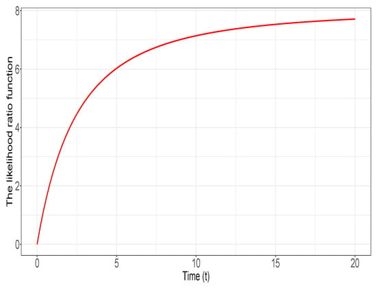
Let us have a cold standby system with size $n=2$ heterogenous components with lifetimes $X_1$ and $X_2$ so that $X_1$ has an arbitrary lifetime distribution ($F_{X_1}\left(0^{-}\right)=0$) and $X_2$ has an exponential lifetime distribution with parameter ${\lambda }_2$, and we, further, assume that $X_1$ and $X_2$ are independent. Then, since

$$S_{1,X{̠}_t}+t{=}_{lr}{X}_{1,t}+t{=}_{lr}{X}_1\left(t\right){\ge }_{lr}{X}_1,$$

then the likelihood ratio ordering in Equation (20) holds true for $n=2$, and hence by Theorem 3, one concludes that $X_{1,t}+X_{2,t}{\ge }_{lr}{(X_1+X_2)}_t$ for all $t\ge 0$. Let us suppose that $X_1$ has a gamma distribution with ${\alpha }_1=2$ and ${\lambda }_1=3$ and $X_2$ has exponential distribution with ${\lambda }_2=3$ as the age $t=5$ is chosen. By routine calculation, for all $x\ge 0,$ one has

$$f_{X_{1,t}+X_{2,t}}\left(x\right)=\frac{27x}{16}(5+\frac{x}{2})e^{-3x}and{f}_{{(X_1+X_2)}_t}\left(x\right)=\frac{27}{257}{(5+x)}^2{e}^{-3x}.$$

In Figure 2, we plot the graph of the function $LR$ given by

$$LR\left(x\right):=\frac{f_{X_{1,t}+X_{2,t}}\left(x\right)}{f_{{(X_1+X_2)}_t}\left(x\right)}=\frac{257x(10+x)}{32{(5+x)}^2}$$

Figure 2. Plot of the likelihood ratio $LR\left(x\right):=\frac{f_{X_{1,t}+X_{2,t}}\left(x\right)}{f_{{(X_1+X_2)}_t}\left(x\right)}$ for $t=5$.

The function $LR\left(x\right)$ is increasing with respect to $x\ge 0,$ according to Theorem 3, and Figure 2 confirms it.

Now, we prove another result to compare the lifetime of a used standby system with the lifetime of another system composed of used components with respect to the usual stochastic order. The following lemma is essential to our development.

Lemma 4.

Let $X̠=(X_1,X_2,\dots ,X_n)$ be a random vector with non-negative random components with joint pdf $f_{X̠}(x̠)$. Fix $l\in \{1,2,\dots ,n\}$. Let $Y̠=(Y_1,Y_2,\dots ,Y_n)$ be another random vector with joint pdf

$$f_{Y̠}(\underset{¯}{y})=\frac{f_{X_l}(t+S_{n,\underset{¯}{y}})}{f_{X_l}(S_{n,\underset{¯}{y}})c(t,l)}{f}_{X̠}\left(\underset{¯}{y}\right),$$

(24)

where $c(t,l)=E\left(\frac{f_{X_l}(t+S_{n,X̠})}{f_{X_l}\left(S_{n,X̠}\right)}\right)<+\infty$. Then, $S_{n,X̠}^l{=}_{st}{S}_{n,Y̠}$, where $S_{n,X̠}^l$ is an rv with pdf $f_{S_{n,X̠}^l}\left(s\right)=\frac{f_{X_l}(t+s)}{f_{X_l}\left(s\right)c(t,l)}{f}_{S_{n,X̠}}\left(s\right)$.

Proof. 

We show that $S_{n,\mathrm{X}̠}^l$ and $S_{n,\mathrm{Y}̠}$ have the same cdf. It is notable that for any function $\beta :\mathbb{R}\mapsto \mathbb{R},$ one has

$$E\left[\beta \left(S_{n,\mathrm{X}̠}^l\right)\right]=\frac{1}{c(t,l)}E\left(\beta \left(S_{n,\mathrm{X}̠}\right)\frac{f_{X_l}(t+S_{n,\mathrm{X}̠})}{f_{X_l}\left(S_{n,\mathrm{X}̠}\right)}\right).$$

(25)

For all $s\ge 0$, one one hand, we can derive

$$P(S_{n,\mathrm{Y}̠}\le s)=\frac{F_{S_{n,\mathrm{X}̠}}\left(s\right)}{c(t,l)}E\left(\frac{f_{X_l}(t+S_{n,\mathrm{X}̠})}{f_{X_l}\left(S_{n,\mathrm{X}̠}\right)}\mid S_{n,\mathrm{X}̠}\le s\right).$$

On the other hand, for all $s\ge 0$, one has

$$\begin{array}{cc}\hfill P(S_{n,\mathrm{X}̠}^l\le s)& =\frac{1}{c(t,l)}{\int }_0^s\frac{f_{X_l}(t+s^{\prime })}{f_{X_l}\left(s^{\prime }\right)}{f}_{S_{n,\mathrm{X}̠}}\left(s^{\prime }\right)d{s}^{\prime }\hfill \\ \hfill & =\frac{F_{S_{n,\mathrm{X}̠}}\left(s\right)}{c(t,l)}{\int }_0^s\frac{f_{X_l}(t+s^{\prime })}{f_{X_l}\left(s^{\prime }\right)}\frac{f_{S_{n,\mathrm{X}̠}}\left(s^{\prime }\right)}{F_{S_{n,\mathrm{X}̠}}\left(s\right)}d{s}^{\prime }\hfill \\ \hfill & =\frac{F_{S_{n,\mathrm{X}̠}}\left(s\right)}{c(t,l)}E\left(\frac{f_{X_l}(t+S_{n,\mathrm{X}̠})}{f_{X_l}\left(S_{n,\mathrm{X}̠}\right)}\mid S_{n,\mathrm{X}̠}\le s\right).\hfill \end{array}$$

The proof of the result is complete. □

We introduce some notation before stating the result. Let $f_Z\left(t\right)$ be the density of the rv Z, which is differentiable. The function ${\eta }_Z\left(t\right)=-\frac{f_Z^{\prime }\left(t\right)}{f_Z\left(t\right)}$ is well-known as the Glaser’s eta function which is very useful in the study of the shape of the hazard rate function and the mean residual life function (see, e.g., Glaser [33] and Gupta and Viles [34]).

Theorem 4.

Let $X_1,X_2,\dots ,X_n$ be independent rvs which are non-negative whose densities are differentiable and $X_{1,t},X_{2,t},\dots ,X_{n,t}$ be also independent, for a fixed $t>0$. Then, if there exists an $l\in \{1,2,\dots ,n\}$ such that

(i)

${\eta }_{S_{n,X̠}}(t+x)-{\eta }_{S_{n,X̠}}\left(x\right)\ge {\eta }_{X_l}(t+x)-{\eta }_{X_l}\left(x\right),$ for all $x\ge 0;$

(ii)

${\eta }_{X_l}(t+x)-{\eta }_{X_l}\left(x\right)$ is increasing in $x\ge 0;$

(iii)

${\eta }_{X_i}(t+x)-{\eta }_{X_i}\left(x\right)\le {\eta }_{X_l}(t+x)-{\eta }_{X_l}\left(x\right),$ for every $i=1,2,\dots n$ and for all $x\ge 0;$

we have

$${\left(S_{n,X̠}\right)}_t{\le }_{st}{S}_{n,X{̠}_t}.$$

(26)

Proof. 

Under the assumption (i), it is found that $\frac{f_{S_{n,\mathrm{X}̠}}(t+x)f_{X_l}\left(x\right)}{f_{S_{n,\mathrm{X}̠}}\left(x\right)f_{X_l}(t+x)}$ is decreasing in $x\ge 0.$ Thus, from Theorem 3.2.(a) of Misra et al. [35], ${\left(S_{n,\mathrm{X}̠}\right)}_t{\le }_{lr}{S}_{n,\mathrm{X}̠}^l$, and, therefore, ${\left(S_{n,\mathrm{X}̠}\right)}_t{\le }_{st}{S}_{n,\mathrm{X}̠}^l$. Suppose now that $n=2$. Note that the assumption (ii) is equivalent to $\frac{f_{X_l}(t+x)}{f_{X_l}\left(x\right)}$ being a log-concave function in $x\ge 0$. By Lemma 4 and Equation (24), there exist non-negative rvs $Y_1$ and $Y_2$ with joint pdf

$$f_{(Y_1,Y_2)}(y_1,y_2)=\frac{f_{X_l}(t+S_{2,\underset{¯}{\mathrm{y}}})}{f_{X_l}\left(S_{2,\underset{¯}{\mathrm{y}}}\right)c(t,l)}{f}_{(X_1,X_2)}(y_1,y_2),$$

(27)

so that $S_{2,\mathrm{X}̠}^l{=}_{st}{Y}_1+Y_2.$ By (27), since $X_1$ and $X_2$ are independent, then $Y_1$ follows the pdf

$$f_{Y_1}\left(y\right)=C_0{f}_{X_1}\left(y\right)E\left(\frac{f_{X_l}(t+y_1+X_2)}{f_{X_l}(y_1+X_2)}\right),y_1\ge 0;$$

where $C_0$ is the normalizing constant. Suppose that $X_i^l$ is an rv with pdf $f_{X_i^l}\left(x\right)=C_1\frac{f_{X_l}(t+x)}{f_{X_l}\left(x\right)}{f}_{X_i}\left(x\right)$ for every $i=1,2$. We can then write

$$\frac{f_{Y_1}\left(y_1\right)}{f_{X_1^l}\left(y_1\right)}=C_{2}E\left(\frac{f_{X_l}(t+y_1+X_2)f_{X_l}\left(y_1\right)}{f_{X_l}(y_1+X_2)f_{X_l}(t+y_1)}\right),$$

in which $C_2$ is the normalizing constant. This ratio is decreasing in $y_{\ge }0$ since $\frac{f_{X_l}(t+x)}{f_{X_l}\left(x\right)}$ is a log-concave function in $x\ge 0$. This is equivalent to saying that $Y_1{\le }_{lr}{X}_1^l,$ and, therefore,

$$Y_1{\le }_{st}{X}_1^l.$$

(28)

Once again, in the spirit of (27), given that $Y_1=y,$ the conditional pdf of $Y_2$ is derived as

$$f_{Y_2|Y_1}\left(y_2\right|y_1)=\frac{f_{X_2}(t+y_1+y_2)f_{X_2}\left(y_2\right)}{f_{X_2}(y_1+y_2)E\left(\frac{f_{X_2}(t+y_1+X_2)}{f_{X_2}(y_1+X_2)}\right)}.$$

For any fixed $y_1\ge 0,$ the log-concavity of $\frac{f_{X_2}(t+x)}{f_{X_2}\left(x\right)}$ in $x\ge 0$ implies that $\frac{f_{Y_2|Y_1}\left(y_2\right|y_1)}{f_{X_2^l}\left(y_2\right)}$ is decreasing in $y_2\ge 0$; that is, $\left[Y_2\right|Y_1=y_1]{\le }_{lr}{X}_2^l$ Thus,

$$\left[Y_2\right|Y_1=y_1]{\le }_{st}{X}_2^l.$$

(29)

Now, taking into account the ordering relations in (28) and (29) and using Theorem 6.B.3 in Shaked and Shanthikumar [27], we obtain $S_{2,\mathrm{X}̠}^l{\le }_{st}{S}_{2,\mathrm{X}{̠}^l},$ where $S_{n,\mathrm{X}{̠}^l}={\sum }_{i=1}^n{X}_i^l,$ for every $n=1,2,\dots$. We use the induction method and assume that

$$S_{n,\mathrm{X}̠}^l{\le }_{st}{S}_{n,\mathrm{X}{̠}^l}$$

(30)

holds true for $n=m\ge 2,$ i.e., $S_{m,\mathrm{X}̠}^l{\le }_{st}{S}_{m,\mathrm{X}{̠}^l}$. From known properties of the usual stochastic order

$$S_{m+1,\mathrm{X}̠}^l{\le }_{st}{S}_{m,\mathrm{X}̠}^l+X_{m+1}^l{\le }_{st}{S}_{m,\mathrm{X}{̠}^l}+X_{m+1}^l{=}_{st}{S}_{m+1,\mathrm{X}{̠}^l},$$

which means that (30) stands valid for $n=m+1$. Thus, we proved that $S_{n,\mathrm{X}̠}^l{\le }_{st}{S}_{n,\mathrm{X}{̠}^l}$.

Since the assumption (iii) means that $f_{X_l}(t+x)f_{X_i}\left(x\right)/f_{X_l}\left(x\right)f_{X_i}(t+x)$ is decreasing in $x\ge 0$, then an application of Theorem 3.2.(a) of Misra et al. [35] implies that $X_i^l{\le }_{lr}{X}_i^t,$ so $X_i^l{\le }_{st}{X}_i^t$ for all $i=1,2,\dots ,n$. Note that $X_i^t{=}_{st}{X}_{i,t},i=1,2,\dots ,n$ where $X_{i,t}{=}_{st}[X_i-t|X_i>t]$ is the residual lifetime after age $t\ge 0$. From Theorem 1.A.3.(b) in Shaked and Shanthikumar [27], it follows that $S_{n,\mathrm{X}{̠}^l}{\le }_{st}{S}_{n,\mathrm{X}{̠}_t}$. Hence, the result is proved. □

The next example clarifies that the property where a standby system composed of used components has a greater reliability than a used standby system is fulfilled in the context of $DLR$ lifetime components distribution.

Example 3.

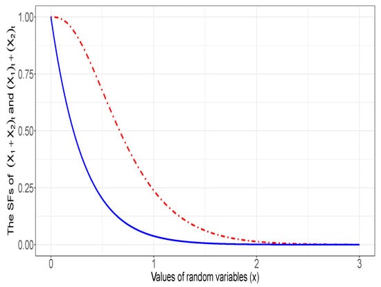
We consider components with heterogeneous independent lifetime distributions. Suppose that $X_i\sim G({\alpha }_i,\lambda ),i=1,2,\dots ,n$. Note that as $X_1,X_2,\dots ,X_n$ are independent rvs, then, consequently, $S_{n,X̠}\sim G({\sum }_{i=1}^n{\alpha }_i,\lambda )$; thus, $f_{S_{n,X̠}}\left(x\right)=\frac{{\lambda }^{{\sum }_{i=1}^n{\alpha }_i}{x}^{{\sum }_{i=1}^n{\alpha }_i-1}{e}^{-\lambda x}}{\mathsf{\Gamma }\left({\sum }_{i=1}^n{\alpha }_i\right)}$. We assume that ${\alpha }_i\le 1$ for all $i=1,2,\dots ,n$ and that ${\alpha }_l={max}_{1\le i\le n}\left\{{\alpha }_i\right\}$. Therefore,

$${\eta }_{X_i}\left(x\right)=\frac{1-{\alpha }_i}{x}+\lambda ,{\eta }_{S_{n,X̠}}\left(x\right)=\frac{1-{\sum }_{i=1}^n{\alpha }_i}{x}+\lambda .$$

For all $x\ge 0,$ it is seen that

$$\begin{array}{cc}{\eta }_{S_{n,X̠}}(t+x)-{\eta }_{S_{n,X̠}}\left(x\right)\hfill & =\frac{t({\sum }_{i=1}^n{\alpha }_i-1)}{x(t+x)}\hfill \end{array}$$

(31)

$$\begin{array}{cc}\hfill & \ge \frac{t({\alpha }_l-1)}{x(t+x)}={\eta }_{X_l}(t+x)-{\eta }_{X_l}\left(x\right).\hfill \end{array}$$

(32)

Thus, the assumption (i) in Theorem 4 holds true. It is further observed that ${\eta }_{X_l}(t+x)-{\eta }_{X_l}\left(x\right)=\frac{({\alpha }_l-1)t}{x(t+x)}$, which is an increasing function in $x\ge 0$, that is, the assumption (ii) in Theorem 4 is satisfied. Since ${\alpha }_i\le {\alpha }_l$ for all $i=1,2,\dots ,n$, then the assumption (iii) in Theorem 4 is also valid, and, consequently, ${\left(S_{n,X̠}\right)}_t{\le }_{st}{S}_{n,X{̠}_t}$. In Figure 3, for better understanding of the result, we plot the graph of rfs of ${\left(S_{n,X̠}\right)}_t$ and $S_{n,X{̠}_t}$ in the special case when $n=3,\lambda =4,{\alpha }_i=1,$$i=1,2,3$, and $t=2$.

Figure 3. Plot of the rf of $S_{2,\mathrm{X}{̠}_t}$ (dot-dashed line) and the rf of ${\left(S_{n,\mathrm{X}̠}\right)}_t$ (solid line) for $t=2$ and for values $x\in (0,3)$ of random variables.

4. Concluding Remarks

With this work we achieved two goals. The first is to develop some stochastic upper bounds on the random lifetime of a cold standby system that is not fresh or new and has age t, having been in operation and still functioning by time t. Two well-known stochastic orders, namely, the likelihood ratio order and a weaker stochastic order, the usual stochastic order, were applied to obtain the stochastic upper bound. The interesting point is that the rf of the lifetime of the used cold standby system with n units is always dominated (without any further assumptions) by the rf of the lifetime of a cold standby system with $(n-1)$ units consisting of used components with common age t, provided that the lifetimes of the used components are shifted t times, as is the case, for example, in the burn-in process. For example, maybe the case in the burn-in process, where a product is placed into use for a time interval of length t before being handed over to the customer, is a realistic situation. However, the domination of this stochastic upper bound over the lifetime of the cold standby system used in terms of the likelihood ratio order requires the further assumption that the components have the $ILR$ property. The second objective was to find conditions under which the lifetime of a used cold standby system with an age of t is dominated by the lifetime of a cold standby unit with used components, each with an age of t, in terms of the likelihood ratio order and the usual stochastic order. In general, and as confirmed by our research as a whole, it is found that the use of cold standby units that were previously in use for an equally long period of time (e.g., t) is preferable to a used cold standby system with age t because it satisfies larger stochastic lifetimes. Therefore, a cold standby system with components $X_{1,t},X_{2,t},\dots ,X_{n,t}$ that has random lifetime $X_{1,t}+X_{2,t}+\dots +X_{n,t}$ is more reliable than a used cold standby system with random lifetime ${(X_1+X_2+\dots +X_n)}_t$ in most situations. We hope that the research conducted in this study will be useful to engineers and system designers.

In the future study, we will use the hazard rate order and the reversed hazard rate order to determine new bounds on the rf and the cumulative distribution function, respectively, of a second-hand cold standby system. We will look for conditions under which the lifetime of a used cold standby system of age t is dominated by the lifetime of a cold standby unit with used components each of age t, in terms of new stochastic orders. Stochastic comparisons between the inactivity times of cold standby systems according to known standard stochastic orders are another problem that can be studied in future work. The importance of the loss caused by further inactivity of engineering systems may motivate us to conduct the above study to design an optimal cold standby unit with less stochastic inactivity. In a future study, one might consider extending this study to applications of reliability-driven design in various areas of engineering optimization, which would provide valuable insights for practitioners and researchers (see, e.g., Baiges [36], Mellal and Zio [37], and Habashneh and Rad [38]).

References

- Kumar, A.; Agarwal, M. A review of standby redundant systems. IEEE Trans. Reliab. 1980, 29, 290–294. [Google Scholar] [CrossRef]
- Kuo, W.; Zuo, M.J. Optimal Reliability Modeling: Principles and Applications; John Wiley and Sons: Hoboken, NJ, USA, 2003. [Google Scholar]
- Yang, G. Life Cycle Reliability Engineering; John Wiley and Sons: Hoboken, NJ, USA, 2007. [Google Scholar]
- Peng, R.Z.; Zhai, Q.; Yang, J. Reliability Modelling and Optimization of Warm Standby Systems; Springer: Singapore, 2022. [Google Scholar]
- Coit, D.W. Cold-standby redundancy optimization for nonrepairable systems. Iie Trans. 2001, 33, 471–478. [Google Scholar] [CrossRef]
- Yu, H.; Yalaoui, F.; Châtelet, Ė.; Chu, C. Optimal design of a maintainable cold-standby system. Reliab. Eng. Syst. Saf. 2007, 92, 85–91. [Google Scholar] [CrossRef]
- Jia, J.; Wu, S. Optimizing replacement policy for a cold-standby system with waiting repair times. Appl. Math. Comput. 2009, 214, 133–141. [Google Scholar] [CrossRef]
- Xing, L.; Tannous, O.; Dugan, J.B. Reliability analysis of nonrepairable cold-standby systems using sequential binary decision diagrams. IEEE Trans. Syst. Man-Cybern.-Part A Syst. Humans 2011, 42, 715–726. [Google Scholar] [CrossRef]
- Ram, M.; Singh, S.B.; Singh, V.V. Stochastic analysis of a standby system with waiting repair strategy. IEEE Trans. Syst. Man, Cybern. Syst. 2013, 43, 698–707. [Google Scholar] [CrossRef]
- Azaron, A.; Perkgoz, C.; Katagiri, H.; Kato, K.; Sakawa, M. Multi-objective reliability optimization for dissimilar-unit cold-standby systems using a genetic algorithm. Comput. Oper. Res. 2009, 36, 1562–1571. [Google Scholar] [CrossRef]
- Wang, C.; Xing, L.; Amari, S.V. A fast approximation method for reliability analysis of cold-standby systems. Reliab. Eng. Syst. Saf. 2012, 106, 119–126. [Google Scholar] [CrossRef]
- Wang, W.; Xiong, J.; Xie, M. A study of interval analysis for cold-standby system reliability optimization under parameter uncertainty. Comput. Ind. Eng. 2016, 97, 93–100. [Google Scholar] [CrossRef]
- Behboudi, Z.; Borzadaran, G.M.; Asadi, M. Reliability modeling of two-unit cold standby systems: A periodic switching approach. Appl. Math. Model. 2021, 92, 176–195. [Google Scholar] [CrossRef]
- Boland, P.J.; El-Neweihi, E. Component redundancy vs system redundancy in the hazard rate ordering. IEEE Trans. Reliab. 1995, 44, 614–619. [Google Scholar] [CrossRef]
- Li, X.; Zhang, Z.; Wu, Y. Some new results involving general standby systems. Appl. Stoch. Model. Bus. Ind. 2009, 25, 632–642. [Google Scholar] [CrossRef]
- Eryilmaz, S. On the mean residual life of a k-out-of-n: G system with a single cold standby component. Eur. J. Oper. Res. 2012, 222, 273–277. [Google Scholar] [CrossRef]
- Eryilmaz, S. The effectiveness of adding cold standby redundancy to a coherent system at system and component levels. Reliab. Eng. Syst. Saf. 2017, 165, 331–335. [Google Scholar] [CrossRef]
- Roy, A.; Gupta, N. Reliability of a coherent system equipped with two cold standby components. Metrika 2020, 83, 677–697. [Google Scholar] [CrossRef]
- Roy, A.; Gupta, N. Reliability function of k-out-of-n system equipped with two cold standby components. Commun.-Stat.-Theory Methods 2021, 50, 5759–5778. [Google Scholar] [CrossRef]
- Gupta, N. Stochastic comparisons of residual lifetimes and inactivity times of coherent systems. J. Appl. Probab. 2013, 50, 848–860. [Google Scholar] [CrossRef]
- Li, X.; Pellerey, F.; You, Y. On used systems and systems with used components. In Stochastic Orders in Reliability and Risk: In Honor of Professor Moshe Shaked; Springer: New York, NY, USA, 2013; pp. 219–233. [Google Scholar]
- Hazra, N.K.; Nanda, A.K. Stochastic comparisons between used systems and systems made by used components. IEEE Trans. Reliab. 2015, 65, 751–762. [Google Scholar] [CrossRef]
- Zhao, P.; Balakrishnan, N. Mean residual life order of convolutions of heterogeneous exponential random variables. J. Multivar. Anal. 2009, 100, 1792–1801. [Google Scholar] [CrossRef]
- Amiri, L.; Khaledi, B.E.; Samaniego, F.J. On skewness and dispersion among convolutions of independent gamma random variables. Probab. Eng. Inf. Sci. 2011, 25, 55–69. [Google Scholar] [CrossRef]
- Khaledi, B.E.; Amiri, L. On the mean residual life order of convolutions of independent uniform random variables. J. Stat. Plan. Inference 2011, 141, 3716–3724. [Google Scholar] [CrossRef]
- Amiripour, F.; Khaledi, B.E.; Shaked, M. Stochastic orderings of convolution residuals. Metrika 2013, 76, 559–576. [Google Scholar] [CrossRef]
- Shaked, M.; Shanthikumar, J.G. (Eds.) Stochastic Orders; Springer: New York, NY, USA, 2007. [Google Scholar]
- Bagnoli, M.; Bergstrom, T. Log-concave probability and its applications. In Rationality and Equilibrium: A Symposium in Honor of Marcel K. Richter; Springer: Berlin/Heidelberg, Germany, 2006; pp. 217–241. [Google Scholar]
- Karlin, S. Total Positivity; Stanford University Press: Redwood, CA, USA, 1968; Volume 1. [Google Scholar]
- Kayid, M.; Alshagrawi, L. Reliability aspects in a dynamic time-to-failure degradation-based model. Proc. Inst. Mech. Eng. Part O J. Risk Reliab. 2022, 236, 968–980. [Google Scholar] [CrossRef]
- Izadkhah, S.; Rezaei, A.H.; Amini, M.; Mohtashami Borzadaran, G.R. A general approach for preservation of some aging classes under weighting. Commun.-Stat.-Theory Methods 2013, 42, 1899–1909. [Google Scholar] [CrossRef]
- Misra, N.; van der Meulen, E.C. On stochastic properties of m-spacings. J. Stat. Plan. Inference 2003, 115, 683–697. [Google Scholar] [CrossRef]
- Glaser, R.E. Bathtub and related failure rate characterizations. J. Am. Stat. Assoc. 1980, 75, 667–672. [Google Scholar] [CrossRef]
- Gupta, R.C.; Viles, W. Roller-coaster failure rates and mean residual life functions with application to the extended generalized inverse Gaussian model. Probab. Eng. Informational Sci. 2011, 251, 103–118. [Google Scholar] [CrossRef]
- Misra, N.; Gupta, N.; Dhariyal, I.D. Preservation of some aging properties and stochastic orders by weighted distributions. Commun. Stat. Theory Methods 2008, 37, 627–644. [Google Scholar] [CrossRef]
- Baiges, J.; Martínez-Frutos, J.; Herrero-Pérez, D.; Otero, F.; Ferrer, A. Large-scale stochastic topology optimization using adaptive mesh refinement and coarsening through a two-level parallelization scheme. Comput. Methods Appl. Mech. Eng. 2019, 343, 186–206. [Google Scholar] [CrossRef]
- Mellal, M.A.; Zio, E. System reliability-redundancy optimization with cold-standby strategy by an enhanced nest cuckoo optimization algorithm. Reliab. Eng. Syst. Saf. 2020, 201, 106973. [Google Scholar] [CrossRef]
- Habashneh, M.; Rad, M.M. Reliability based topology optimization of thermoelastic structures using bi-directional evolutionary structural optimization method. Int. J. Mech. Mater. Des. 2023, 25, 1–16. [Google Scholar] [CrossRef]
Disclaimer/Publisher’s Note: The statements, opinions and data contained in all publications are solely those of the individual author(s) and contributor(s) and not of MDPI and/or the editor(s). MDPI and/or the editor(s) disclaim responsibility for any injury to people or property resulting from any ideas, methods, instructions or products referred to in the content. |
© 2023 by the authors. Licensee MDPI, Basel, Switzerland. This article is an open access article distributed under the terms and conditions of the Creative Commons Attribution (CC BY) license (https://creativecommons.org/licenses/by/4.0/).