Mathematical Analysis of the Reliability of Modern Trolleybuses and Electric Buses

Abstract

The rhythmic and stable operation of trolleybuses and autonomous trolleybuses or urban electric buses, depends to a large extent on the reliability of the equipment installed on the trolleybus. The actual operational reliability of trolleybus electrical equipment (EE) depends on its technical condition. Under the influence of external factors and specific operating modes, the technical condition of the equipment is continuously deteriorating, reliability indicators are decreasing, and the number of failures is increasing. Using the mathematical theory of reliability, probability theory and mathematical statistics, numerical methods of solving nonlinear and transcendental equations, this article defines the conditions of diagnostics depending on the intensity of failures and the given probability of failure-free operation of the equipment. Additionally, the inverse problem of determining the current reliability of electrical engineering systems depends on the terms of diagnostics and the intensity of failures being solved. As a result of the processing of statistical information on failures it is established that for the electrical equipment of a trolleybus, after a number of repair measures, the maximum density of failures occurs at a lower mileage, and the probability of failure-free operation can vary depending on the degree of wear of the equipment, i.e., on the number of previous failures. It is theoretically substantiated and experimentally confirmed that the reliability of trolleybus electrical equipment changes according to the exponential law of distribution of a random variable. It has been established that the real averaged diagnostic terms regulated by instructions are not optimal in most cases and differ several times from those defined in this paper. The dependence of switching equipment run-in on time has been clarified, which served as a prerequisite for specifying the inter-repair period for various types of trolleybus electrical equipment. A method of adjustment of the inter-repair time for the electrical equipment of trolleybuses is proposed.

1. Introduction

The development of passenger, urban transport is subject to the laws of settlement, which, in turn, depends on the improvement of transport facilities and infrastructure [1]. In recent decades, the increasing process of suburbanization in developed countries has led to a reduction in the share of labor trips from the suburbs to the cities (in the U.S.—from 35 to 10%). In Europe, along with trips by car (50% of trips), movement by public transport (bus, subway, urban railroads—more than 20%), as well as by bicycles, mopeds, walking—about 30% of movements are more and more common [2]. On the whole, in the sphere of communications, city transport is competed with by modern information technologies, the development of which leads to a reduction in the need for business (by 20 to 25%) in developed countries and cultural and household (by 50%) trips [3]. These outlined trends in the development of world transport will be decisive in the future. Among the main trends, in addition to the traditional ones—increasing the speed, capacity, freight capacity, environmental friendliness, the appearance of new vehicles and new types of messages—it is possible to note an orientation towards the qualitative characteristics demanded by the customer (reliability, rhythm, timeliness of cargo delivery, comfort, safety of passenger travel), as a result the issues of an economic nature (costs, profit, profitability) leaving the category with primary importance [4]. The market of transport services turns into a complex system of interaction with other components in the sphere of delivery, forming transport and storage, goods transportation and distribution logistic complexes with the use of the latest information systems, modeling, marketing with further connection to the system of the banking sphere, i.e., formation of a single system of exchange of goods, capital, and information [5]. The desire to improve the competitiveness of the national transport system and its individual types is accompanied by the formation of a unified world transport system with harmonization of laws, common to all participants in the transport process [6]. At the same time, the complexity, quantitative growth and qualitative changes in the market of transport services leads to the emergence of risks, and contradictions as world transport develops, making more vulnerable not only the sphere of movement, but also the economic and social components of the lives of the population [7].

Improvement of mathematical methods of reliability research is of fundamental importance for operational organization of transport systems [8]. Reliability analysis allows the development of a set of measures to improve reliability and durability of both separate elements and trolleybuses as a whole, to substantiate the system of maintenance and repair, to estimate the real level of failure-free operation, and to form reliability requirements in relation to the given operating conditions [9]. Unfortunately, the known methods of research of the reliability of complex systems used in radio electronics, automatics, electrical power engineering, are not always applicable to electromechanical systems [4]. Such peculiarity is connected with the operation of the above-described systems. Any complex system of automatics and radio electronics consists of standard elements (resistors, capacitors, diodes, transistors, etc.) with stable reliability indicators [2,5]. There is no need for the study of the aging processes of such elements, because in the case of failure of such elements they are replaced with spare ones.

Design of electrical machines requires a different approach to safety and durability of assembly units and parts, as replacement of elements with spare ones is rather labor-intensive in some cases [6]. It is necessary to take into account the aging of insulating materials, wear resistance of bearings, etc. The ageing processes in electrical machines (EM) lead to the necessity of their repair following use [10].

Application of mathematical statistical methods for the definition of reliability indicators is required by the lack of a definition of the technical resource for each concrete trolleybus motor [11]. This peculiarity is connected with the ageing of the winding insulation during heating, which is always present during operation. Additionally, we should not forget about environmental conditions, which significantly affect the aging processes of materials. The described processes cannot be controlled by methods of technical diagnostics.

Application of technical diagnostics for electric traction motors (TED) is possible in order to estimate bearing and lubrication life, but their reliability indicators are not the weakest links [10]. Satisfactory condition of these elements is evaluated during scheduled maintenance.

In cases when it is impossible to determine the characteristics of the aging processes, the probability distribution parameters have to be established by statistical processing of experimental data. It should be noted that statistical modeling makes it possible to investigate the actual reliability of products according to in-service observation data. In this case it is necessary to determine the average operating time and service life before repair, operating time to failure, availability coefficients and other actual reliability indicators [11,12,13].

In order to maintain the required level of reliability of a trolleybus as a whole, it is necessary to carry out an engineering analysis. The engineering analysis consists of two main stages:

(1)

identify “weak links” of trolleybus electrical equipment and get an actual picture of the reliability of elements;

(2)

carry out a reliability study of the traction electric motor on the basis of failure analysis.

Operational reliability of the traction electric motor depends on the operational reliability parameters of its following elements: stator winding, rotor winding, bearing device [14,15].

Reliability of the mechanical EE of vehicles has been widely studied in the automotive industry, aviation, railway transport, and agricultural machinery. At the same time, a patent information search shows that the EE reliability of trolleybus and electric bus rolling stock has been little studied and the number of publications on this topic is significantly less compared to the publications on other vehicles [3].

The experience of operating modern trolleybuses and electric buses shows that the cost of maintaining (restoring) reliability is three to six times higher than the cost of creating them with a certain level of reliability [4].

Maintenance and repair of TCEBs currently accounts for up to 75% of all funds of transportation companies spent on the organization of passenger transportation, and the cost of maintenance and repair of the electrical complex of TCEBs is about 60% of the total maintenance costs of the rolling stock.

Considering the fact that the actual operating rolling stock of TCEBs, especially old trolleybuses, is worn out by more than 70%, the problems of ensuring EE reliability during operation and determining the actual technical condition and forecasting it are primary tasks.

The necessary level of EE reliability can be maintained only if its technical condition is systematically monitored and diagnosed, and timely repairs are carried out to prevent a decrease in reliability.

Diagnostics is currently one of the main aims of improvement of EE repair systems, and increase in its reliability of operation, as it contributes to prevention of failures of accidental nature in the periods between repairs. Application of the means and methods of technical diagnostics, allowing continuously or at discrete moments of time to check the state of input and output parameters of TCEBs, makes it possible to repair them in accordance with the actual technical state. This contributes to significant reductions in the number of failures in the period between scheduled repairs, an increase in the degree of use of the resource of assembly units and equipment parts, and an increase in the economy of operation and traffic safety. When diagnosing, it is first necessary to clearly distinguish the object and having analyzed it, determine the signs and parameters, as well as methods and means of diagnosis.

For a more complete assessment of the technical condition of the EE it is necessary to develop a comprehensive approach to reliability assessment and prediction of the EE TCEB’s serviceability by means of technical diagnostics and traceability. This would allow accurate determination of the current technical condition of the EE, monitoring it on the one hand, and predicting changes in the technical condition on the other hand, ensuring with a certain probability that during the period between repairs there will be no failures of the EE due to wear and insufficient reliability.

The effectiveness of the planned preventive maintenance system of TCEBs actually operating at electric transport enterprises at the present time, depends largely on the compliance of the established inter-repair mileage of rolling stock actually necessary, which, in turn, depends on the resources of individual units and components of TCEBs equipment [5].

Planned preventive systems of repairs, are based on the pre-regulated frequency of repairs with the established possible limits of their change for different types of equipment. However, despite this, changes in the technical condition of the equipment, occurring in the process of its operation and modernization are not take into account.

The problem of evaluating the reliability and predicting the performance of the TCEB’s electrical complex involves solving the following problems:

• optimal organization of diagnostics and control of technical condition of EE;
• assessment and prediction of EE reliability during operation;
• Optimization of timing, definition of scope and selection of a rational strategy and planning of maintenance and repair of EE, taking into account its technical condition.

Thus, the basic principle of the new technology of EE technical condition management is the method of EE maintenance and repair, based on individual observation of real changes in the technical condition of equipment during operation [6]. Then, the system of maintenance and repair is a set of rules, providing a given management of production operation of EE based on control of its technical condition.

The aim of the work is to improve the existing and develop new scientifically valid methods and means of assessing the reliability and predicting the performance of trolleybus EE.

The applied nature of the work consists of the development of an integral probabilistic-diagnostic system for monitoring and forecasting the technical condition of electrical complex TCEBs and a method of continuous monitoring and forecasting of the serviceability of equipment on its basis.

In accordance with this goal, the following tasks had to be solved:

• Conducting and systematizing an analysis of existing methods of diagnosing and evaluating the reliability of EE.
• Optimal organization of diagnostic and technical condition control processes of trolleybus EE. Creation of an algorithm for trolleybus EE diagnostics.
• Assessment and prediction of reliability of the trolleybus electrical complex by operational indicators and optimization of EE maintenance timing by mileage and operating time.
• Development of integrated methods for reliability assessment and prediction of serviceability and integral probabilistic diagnostic systems for predicting the technical condition of the trolleybus electrical complex using stochastic and deterministic models.

Trolleybuses and electric buses are complex technical systems. Considering that there are hundreds of systems with a total number of subsystems, units, elements and parts more than ten thousand in a trolleybus and electric bus, it is very important to take into account the mutual influence of these components on each other when determining the reliability of the entire system For example, the authors have experimentally established that failures of the mechanical equipment of electric buses (transmission, gearbox, cardan shafts, etc.) can cause failures and failures of the traction motor. Taking into account these mutual influences not only qualitatively, but also quantitatively with the help of mathematical analysis would allow an increase in the accuracy of determining and predicting the reliability of the electrical equipment of modern trolleybuses and electric buses.

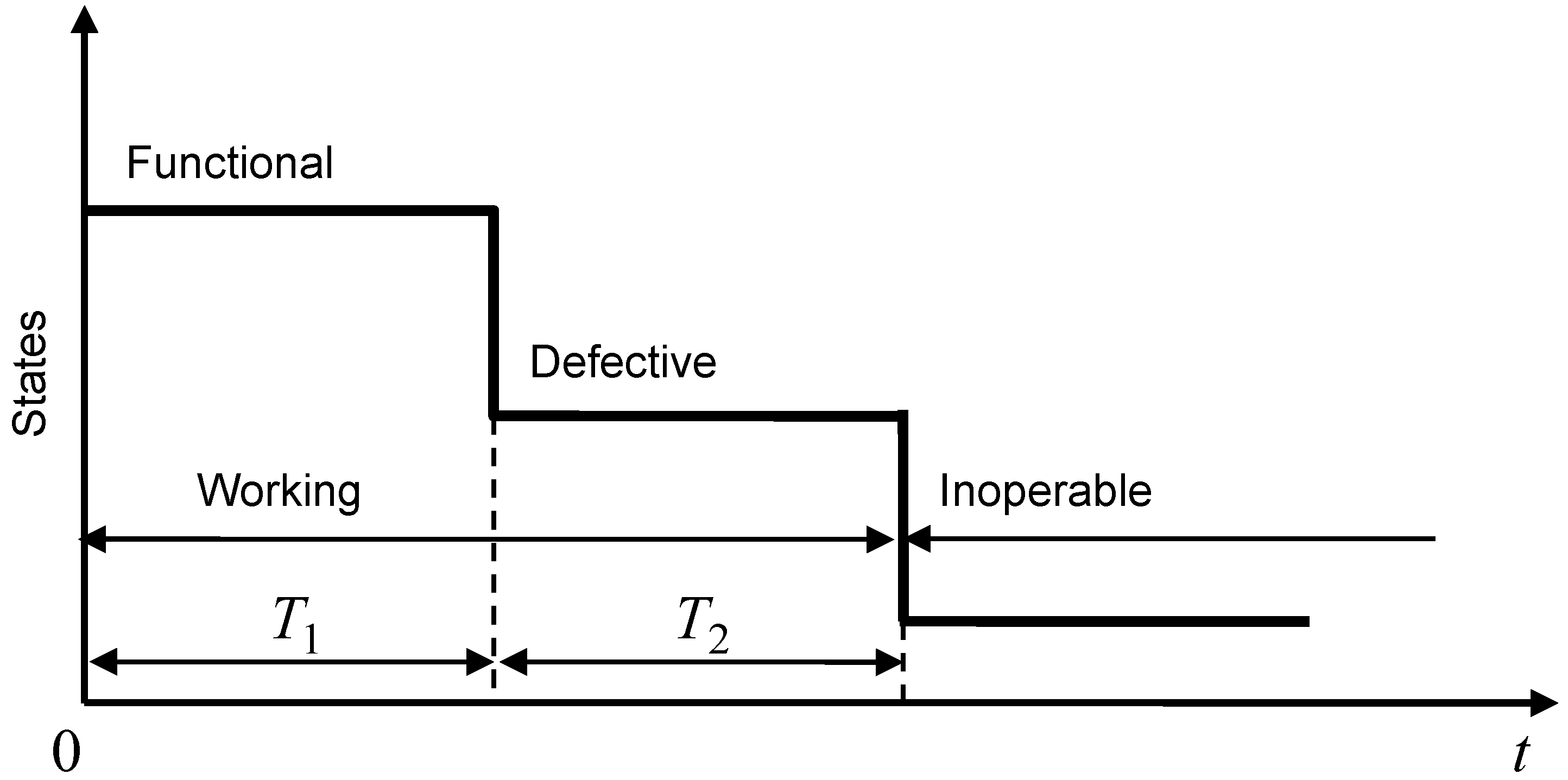
2. Analysis of the Effect of Service Life of Electrical Equipment on the Probability of Failure-Free Operation

Comparing existing methods of reliability analysis and statistical models [7,8,9], it should be noted that mass statistical modeling allows us to study the actual reliability of products according to observations from operation within the framework of those models that the authors have built through the average time to failure and service life before repair, time to failure and the availability factor. The novelty of this work is that we take into account malfunctions that do not lead to failures and that can be promptly eliminated and failures of electrical complexes that lead to non-regular removal from the line of electric rolling stock and their repair while the electric bus should have been on the line. Here we are talking about inter-repair failures—the most undesirable equipment failures. Additionally, the novelty of the presented model is its ability to take into account the fact that when restoring the equipment during the maintenance of the system nodes, the restoration of the whole system is not 100%, and each of its subsequent restorations worsens the indicators of its reliability. Here the resource recovery factor $k_r\in \left[0\dots 1\right]$ is used. The resource recovery factor of an element means the probability of how much resource recovery correlates with a new element, which has a probability of failure-free operation $P\left(t\right)=100\%$.

The main task of the work was to estimate the period of trolleybus EE diagnostics and refine it in comparison to the existing one. The main material for analysis was the statistical material of faults of Novosibirsk depot No. 2 for 2022.

According to [7], inspections of electrical equipment are performed according to the regulations on maintenance No. 0 (maintenance-0) on a calendar schedule (on the 4th or 7th day), and then on a calendar schedule (assuming that the trolleybus mileage is fairly uniform). In this case the preventive maintenance becomes a combined preventive maintenance for the application of rolling stock units. During preventive maintenance, the main goal is to detect a failure that can lead to failure. The state of the control object can be (according to this) one of three (Figure 1).

The main quantitative characteristic of a group of any similar objects (including a group of trolleybus moving units) is reliability or probability of no-failure operation P(t) [8]. It characterizes the most probable share of operable units of this group at the considered moment of time t. The function P(t) is a decreasing one, as the devices wear out. Failure of devices in a given group is characterized by the density or intensity of failures λ(t). The failure rate λ(t) is the probability of failure of a device during the time t, referring to the value of the interval t, provided that the device has worked up to the given interval Δt (it is an a posteriori probability) [9].

To characterize before the device operation, the probability of failure of the device at this or that moment of time, it is convenient to use the distribution density f(t) of time of no-failure operation [10], equal to the unconditional probability of failure in the interval t, referred to the value t. In the course of operation itself the device could fail to reach the proposed point in time, and it could pass the given moment—it is an a priori parameter.

The analytical relationships between these parameters are as follows

$$f\left(t\right)=\raisebox{1ex}{$-dP$}\!\left/ \!\raisebox{-1ex}{$dt$}\right.,$$

(1)

$$\lambda \left(t\right)=\raisebox{1ex}{$f\left(t\right)$}\!\left/ \!\raisebox{-1ex}{$P\left(t\right)$}\right.=-\frac{1}{P\left(t\right)}\cdot P^{\prime }\left(t\right)=\frac{N\left(\Delta t_i\right)}{N_{av i}\cdot \Delta t_i},$$

(2)

where $f\left(t\right)$ is density of distribution of uptime;

• $\lambda \left(t\right)$ is the probability of device failure during the time $\Delta t$;
• $P\left(t\right)$ is reliability or probability of failure;
• $P^{\prime }\left(t\right)$ is the distribution density of uptime;
• $N\left(\Delta t_i\right)$ is the number of failures of similar objects on the interval $\Delta t_i$;
• $N_{av i}$ is number of operable objects in the middle of the interval.

In addition to the considered indicators, such as the mean time of no-failure operation T_av, the unreliability function (probability of failure) [11] is used.

$$Q\left(t\right)=1-P\left(t\right).$$

(3)

When new rolling stock enters the fleet, all its elements are new, and their first failure occurs after some average time T_av1 (or after some average mileage L_av1). The first failures are clustered around T_av1. After the repair action of the failed element, the remaining EE elements continue to age and fail and will create second, third and subsequent failures [12]. These failures will occur faster and faster after a new (from the maintenance action) run begins and gradually the distribution of the frequency of failures from the run will acquire a falling character, which is well approximated by an exponential function. The exponential distribution law is the most well-known and used in practice. It is called the basic law of reliability because it is often used to predict reliability during normal operation of products, when gradual failures have not yet manifested themselves and reliability is characterized by sudden failures. These failures are most often caused by an unfavorable set of circumstances and therefore have a constant intensity. With the exponential law, the probability of failure-free operation depends only on the duration of the time interval and does not depend on the time of previous operation, which is especially important, since in trolleybus and electric buses there are constant replacements of failed units and subsystems with new or reconditioned ones.

Studies conducted in trolleybus depots of large cities—in Novosibirsk, Barnaul, Tomsk, Omsk confirmed the correctness of this theory.

Figure 2 shows the experimental graphs P(L) for traction motors (TED), obtained from a group of 20 trolleybuses participating in the experiment. As can be seen from Figure 2, after a number of maintenance impacts, the maximum failure density occurs at lower mileage.

Figure 2 shows the experimental P(L) plots for TEDs obtained in a group of 30 trolleybuses participating in the experiment. To construct these characteristics, the failure statistics of TEDs were collected, a histogram of equipment failures was constructed, then its cumulant, and the inverse function of failure-free operation P(L) was constructed. As can be seen from Figure 2, after a series of maintenance actions, the maximum failure density occurs at lower mileage, and the probability of failure-free operation can vary depending on the degree of wear of the equipment, i.e., the number of previous failures. The model of change in the probability of failure-free operation P(L) presented in Figure 2 clearly shows that in fact there is no complete restoration of the system reliability to 100%. This is explained by the complexity of the trolleybus technical system, a large number of subsystems, nodes, assemblies and parts and their mutual influence on each other. Traditional statistical models of reliability change from mileage or time do not allow taking into account this mutual influence. In our model we were able to show and obtain quantitative indicators in the form of distribution of failure rate and density of distribution depending on the duration of equipment operation.

It was also found as a result of the analysis of statistical information about failures, that the probability of failure-free operation P(t) or the law of change in reliability EE can vary depending on the degree of wear of equipment, that is, the number of previous failures [13]. The laws of reliability change in trolleybus TEDs depending on their operation term with average operating time of failure T_av = 60 days, and are presented in Figure 3. The normal law (Gauss law, curve 4) is true for brand new TEDs. For TEDs after a small number of failures, Rayleigh’s law or the uniform and exponential law (curves 3, 2, 1) is more accurate.

The largest errors in the initial acceptance of the wrong law can be determined from the graph of the relative error depending on the given reliability [14] (Figure 4). It is established [15] that the existing average reliability of the trolleybus P(t) does not fall below 0.8, then the error in the choice of the law of change in reliability EE for the analysis is about 5%.

Thus, it is possible in future research to take the reliability of EE in operation, and changes according to the exponential law [16]

$$P\left(t\right)=e^{-\lambda \cdot t}\approx e^{\frac{-t}{T_{av}}}.$$

(4)

Failure rate λ of the equipment can be determined by failure statistics as an average value [17]. Assuming that λ remains a constant value, i.e., λ = λ_av, it is known [18,19] that over the period of equipment operation the intensity of its failures changes in accordance with the law of Figure 5. Failure to take into account this pattern in sections I and III will lead to a significant error in assigning a diagnostic period [20,21].

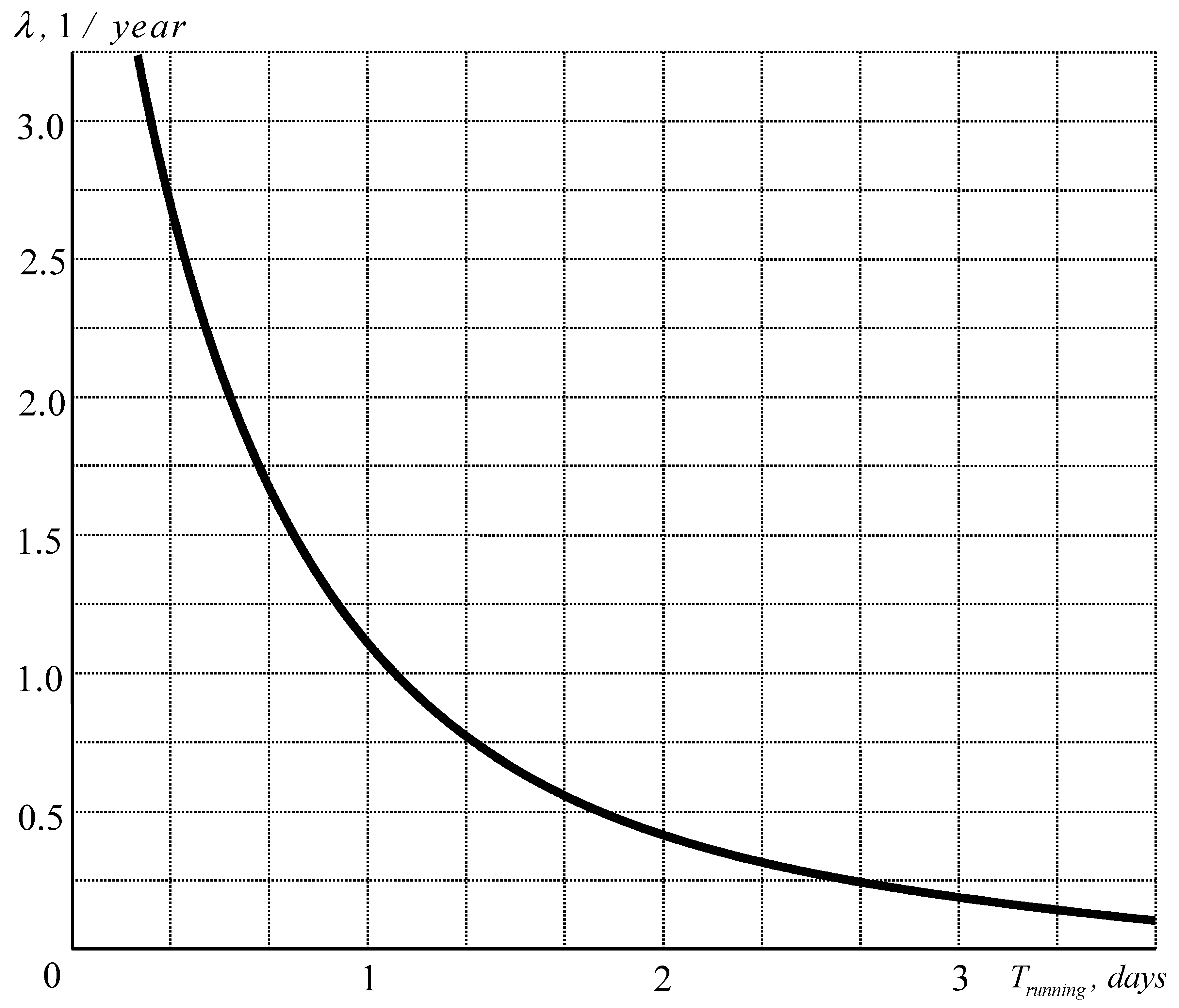
3. Determination of the Timeframe for Diagnosing the Trolleybus Electrical Complex Based on the Mean Time between Failures (MTBF)

If maintenance EE is carried out with restoration of reliability to P(t) ≈ 1 in period I (Figure 5), when the flow of near-working failures has not ended, the intensity of equipment failure will be artificially overestimated. Obviously, the terms of maintenance actions will also be erroneously overestimated.

If during preventive maintenance the reliability was restored to P(t) ≈ 1, the frequency of preventive maintenance is equal to t_d and it is carried out for each of N EE units of one group uniformly with the interval t_d/N, then reliability graphs of each object will look like (Figure 6), where the qualitative dependences for the group of homogeneous objects at N = 5 are given.

Naturally, the assumption of recovery under prevention to P(t) ≈ 1 is an approximation [22].

In the discussed group, the reliability of each k-th object (k = 0, 1, 2, … N − 1), given that the exponential law of reliability prevails when the fleet is worn out, is defined by the expression

$$P_k\left(t\right)=e^{-\frac{t+k\cdot \left(\frac{t_d}{N}\right)}{T}},$$

(5)

where T is the failure time of the k-th element.

In this case, the average reliability function of the whole group consisting of N objects in the interval $t=0\dots \frac{t_d}{N}$ is represented by the expression

$$\overline{P\left(t\right)}=\frac{P_1\left(t\right)+P_2\left(t\right)+\dots +P_k\left(t\right)+\dots +P_N\left(t\right)}{N}.$$

(6)

Writing (6) as the sum of a geometric progression divided by N, we obtain

$$\overline{P\left(t\right)}=\frac{e^{\frac{t_d-N\left(t+t_d\right)}{N\cdot T}}\cdot \left(1-e^{-\frac{t_d}{T}}\right)}{N\cdot \left(1-e^{-\frac{t_d}{N\cdot T}}\right)}.$$

(7)

Thus, the value of the average reliability of the entire group of objects for the year can be analytically determined from (7)

$$\overline{P_{av}}=\frac{{\overline{P\left(t\right)}}_{\mathit{max}}+{\overline{P\left(t\right)}}_{\mathit{min}}}{2}.$$

(8)

For the values of time t = 0 and $t=\frac{t_d}{N}$, determining the maximum and minimum level of reliability of each of the N objects in the group, we will have

$$\left.{\overline{P\left(t\right)}}_{\mathit{max}}=\frac{e^{\frac{t_d\cdot \left(1-N\right)}{N\cdot T}}\cdot \left(1-e^{-\frac{t_d}{T}}\right)}{N\cdot \left(1-e^{-\frac{t_d}{N\cdot T}}\right)} , {\overline{P\left(t\right)}}_{\mathit{min}}=\frac{e^{-\frac{t_d}{T}}\cdot \left(1-e^{-\frac{t_d}{T}}\right)}{N\cdot \left(1-e^{-\frac{t_d}{N\cdot T}}\right)} \right|.$$

(9)

From Equations (8) and (9) at failure rate $\lambda =\frac{1}{T}$, we can get an expression for $\overline{P_{av}}$. As experiments have shown, there are annual fluctuations of the failure parameter [23]. In this connection there are confidence limits, within which the actual value of the failure rate of the element in question can be found. Confidence bounds are defined for the probability of their observance of the following mathematical condition—failures are random phenomena and there is a probability of going out of bounds λ [24]. In this connection, the confidence coefficient α is used. Practically, taking the probability of non-exit of intensity of failures out of the limits of a confidence interval makes 90% (α = 0.9), we define the lower λ_l and the upper λ_u limits of a confidence interval as

$${\lambda }_{l,u}=\frac{\lambda }{r_{1, 2}},$$

(10)

where $r_{1, 2}$ are specially tabulated functions depending on the number of failures m and the coefficient α [25]. Of practical interest is the upper bound of the failure rate, at which the failure rate is maximal [26].

The results of calculation of failure rate λ and mean time between failures T for the Novosibirsk trolleybus depot are given in

Table 1. Failure rate and average MTBF of the trolleybus electrical complex.

No. n/a	Type of Electrical Equipment	λ, 1/Year	Confidence Interval at α = 0.9		T, Year	tdopt, Year × 10−2	kreturns
			λl	λu
1	Circuit breaker (CB)	2.015	1.914	2.156	0.46	2.31	0.225
2	Traction motor (TED)	3.235	3.073	3.461	0.28	0.72	0.218
3	Auxiliary motor (AP)	7.167	6.808	7.668	0.13	0.32	0.322
4	Motor-compressor (MC)	6.123	5.816	6.551	0.15	19.5	0.250
5	Generator (D)	3.055	2.902	3.268	0.30	0.76	0.186
6	Current regulator relay (RRT)	3.414	3.243	3.652	0.27	0.68	0.272
7	Voltage relay (RN)	3.235	3.073	3.461	0.28	0.72	0.274
8	Current relay (CT)	3.305	3.139	3.536	0.27	0.71	0.003
9	Current collectors	9.58	9.101	10.25	0.09	0.16	0.163
10	Control circuit	3.235	3.073	3.461	0.28	0.72	0.139
11	Contactor	17.85	16.95	19.09	0.05	0.13	0.197
12	Starting and shunt resistors	2.575	2.446	2.755	0.36	0.91	0.419
13	Line contactor 4 and 5	1.667	1.583	1.783	0.56	3.08	0.091
14	Leakage current	4.735	4.498	5.066	0.19	0.49	0.393
15	Controller and reverser	4.378	4.159	4.684	0.21	0.53	0.233
16	Battery	4.735	4.498	5.066	0.19	0.85	0.296
17	Pedals	5.405	5.134	5.783	0.17	1.65	0.192
18	Alarm system	0.915	0.869	0.979	1.02	1.75	0.136
19	Servomotor	6.215	5.904	6.650	0.15	0.37	0.135
20	Furnaces and lighting	3.355	3.187	3.589	0.27	0.69	0.187

.

In determining the failure rate and average MTBF of the trolleybus electrical system, failure statistics differentiated by electrical equipment type were collected. For this purpose, the control room system collected daily information on failures of all electrical equipment of the trolleybus and differentiated these failures by the type of electrical equipment presented in Table 1. Then, according to the above formulas, the failure rate and the optimal time for diagnosing the trolleybus equipment were determined.

Using the data in Table 1, we can identify the group of EEs for which significant increases in failure rates are possible: compressor motor, line contactor 5 and 4, circuit breaker, starting and braking resistors, pedals, alarms, batteries.

With unchanged quality of maintenance impacts, the increase in failure rates for the rest of the electrical equipment with a 90% probability will not exceed 10–12% (Table 1).

Using Equation (9) in (8), we obtain an equation that allows us to determine the individual failure rate λ under given operating conditions for the average annual reliability of an object

$${\overline{P}}_{av}=\frac{\left(1-e^{-\frac{t_d}{T}}\right)}{2\cdot N\cdot \left(1-e^{-\frac{t_d}{N\cdot T}}\right)}\cdot \left(e^{\frac{t_{d\cdot \left(1-N\right)}}{N\cdot T}}+e^{-\frac{t_d}{T}}\right),$$

(11)

where $T=\frac{1}{\lambda }$. Equation (11) is transcendental with respect to T, which is solved only by numerical methods [27]. Let us solve it for a single point using the graphical method. Taking into account the smallness of the index $\raisebox{1ex}{$t_d$}\!\left/ \!\raisebox{-1ex}{$N\cdot T$}\right.$ at N = 100 moving units and accepted by [28].

$$e^{-\frac{t_d}{N\cdot T}}\approx 1-\frac{t_d}{T\cdot N},$$

(12)

We get a simpler equation

$${\overline{P}}_{av}=\frac{\left(1-e^{-\frac{t_d}{T}}\right)\cdot \left(e^{\frac{t_{d\cdot \left(1-N\right)}}{N\cdot T}}+e^{-\frac{t_d}{T}}\right)}{2\cdot \frac{t_d}{T}}.$$

(13)

Given that at N = 100 the expression 1 − N ≈ −N, we obtain

$${\overline{P}}_{av}\cdot \frac{t_d}{T}=\left(1-e^{-\frac{t_d}{T}}\right)\cdot e^{-\frac{t_d}{T}}.$$

(14)

Equation (14) is solved graphically by determining the intersection point of the graphs $\left(1-e^{-\frac{t_d}{T}}\right)\cdot e^{-\frac{t_d}{T}}$ and ${\overline{P}}_{av}\cdot \frac{t_d}{T}$.

The graphical solution of Equation (11) is shown in Figure 7. Thus, with certain P = 0.921 and t_d = 3.5, we find T = 20.9.

Using Wolfram research Mathematica (v 10.0.2.) [29] software, the characteristic families t_d and the three-dimensional surface in coordinates (${\overline{P}}_{av}$, T, t_d) were obtained.

Figure 8 shows plots for determining individual operating time to failure at a given reliability of the whole group and restoration time of electrical equipment to P = 1 at t_d = 3.5 days, t_d = 7 days, t_d = 14 days, t_d = 28 days, t_d = 56 days, t_d = 112 days, t_d = 224 days, corresponding to a complete repair cycle. Figure 9 shows the solution of Equation (11) relative to t_d as a three-dimensional surface in coordinates (${\overline{P}}_{av}$, T, t_d) at T = 1 … 1000 days, ${\overline{P}}_{av}=0.1 \dots 0.95$ and t_d = 0 … 1600 days, the data for which are given in

Table 2. Values of individual operating time to failure for given reliability and recovery time of electrical equipment.

${\overline{\mathit{P}}}_{\mathit{a}\mathit{v}}$	T, Days
	td = 3.5	td = 7	td = 14	td = 28	td = 56	td = 112	td = 224
0.01	1.031	2.062	4.131	8.271	16.542	33.084	66.169
0.1	2.164	4.328	8.658	17.316	34.633	69.265	138.53
0.2	3.141	6.2822	12.561	25.122	50.244	100.489	200.98
0.3	4.231	8.462	16.927	33.854	67.709	135.42	270.84
0.4	5.592	11.184	22.368	44.737	89.474	178.95	357.89
0.5	7.424	14.849	29.699	59.397	118.79	237.59	475.18
0.6	10.112	20.224	40.441	80.882	161.76	323.53	647.05
0.7	14.522	29.051	58.091	116.18	232.36	464.72	929.45
0.8	23.272	46.541	93.089	186.18	372.36	744.71	1489.4
0.9	49.392	98.797	197.594	395.19	790.38	1580.8	3161.5
0.99	518.79	1037.6	2075.1	4150.3	8300.6	16,601	33,202

.

Obviously, if the MTBF determined by the most dangerous boundary (Table 1)

$$T_v=\frac{1}{{\lambda }_v}$$

(15)

is a year or its substantial part, then using the graphs of Figure 8 and Figure 9 gives almost the same value as expression (15). For a smaller value of T_v, Figure 8 gives a slightly different, more accurate value of the operating time.

From Figure 8 we can see that for a given time of MTBF for traction motor T₁ = 476 at different values of diagnostic time t_d, for example a traction motor, we will have a different level of its reliability. So, at t_d = 28 days we will have ${\overline{P}}_{av}=0.921$, and at t_d = 7 days we will have ${\overline{P}}_{av}=0.96$. Thus, it is obvious that the reliability of trolleybus electrical equipment increases with decreasing diagnostic time [30,31].

For trolleybus electrical complexes, Figure 10 shows a graph of the relationship between the failure rate λ and the running-in period of trolleybus electrical switching equipment [32]. During the running-in period the objects have a significant frequency of failures. Taking the frequency of failures as a measure of operation intensity, thereby taking into account the quality of service effects and external conditions and factors of operation, the running-in duration of trolleybus switching equipment was determined.

Table 3. Dependence between failure rate λ and running-in time T_running of trolleybus electrical switching equipment.

No. n/a	Name of Equipment	Trunning, Days
1	Circuit breaker (CB)	1.51
2	Regulator relay (RR)	1.24
3	Voltage relay (RN)	1.15
4	Current relay (CT)	1.08
5	Control circuit	1.49
6	Line contactor LK4, LK5	2.20
7	Group rheostat controller and reverser	1.83
8	Control controller	2.15
9	Field weakening contactor	1.71

shows the dependence between the failure rate λ and the running-in time T_running of the trolleybus electrical switching equipment.

Thus, the data obtained with the average preventive time t_d = 7 are overestimated due to a large proportion of the running time in the entire preventive period. Obviously, this conclusion should serve as a prerequisite for a certain specification of the inter-preventive time t_d for each of the trolleybus EE types [33]. At the same time, due to the fact that estimates of the running times are made by the ratio of failures, these values can be slightly increased and, for example, the running time for a repaired field weakening contactor will slightly exceed the time of 1.7 days.

The above practically means that adjustment work, e.g., in an operable control circuit, should not be carried out more often than once every 6 days, since the risk of failure of such adjustment is certainly increased by the fact that the entire control circuit starts to run-in again on its elements. Moreover, in the presence of control circuit failure, it is important to find the truly faulty element without significantly disturbing the operating conditions of other elements that are already running-in, that is, in the mode, according to Figure 5, with a low failure rate.

Naturally, the running-in time should account for a small fraction of the total inter-diagnostic period [34].

So, if the initial running intensity λ is three times higher than the intensity during normal operation of EE, then at the inter-diagnostic period t_d equal to the tripled running time T_running, the average failure intensity will be equal to 1.33λ. This means that the probability per time unit of failure in an EE group due to a large share of not worked-in elements will be increased by 33% relative to the situation when all elements in this group have already been worked-in.

Thus, according to the calculations, for some elements of the trolleybus EE, it is necessary to increase the existing inter-protection period.

To clarify this conclusion, the methods and criteria are set out in the example of the maintenance of aviation electrical equipment [35].

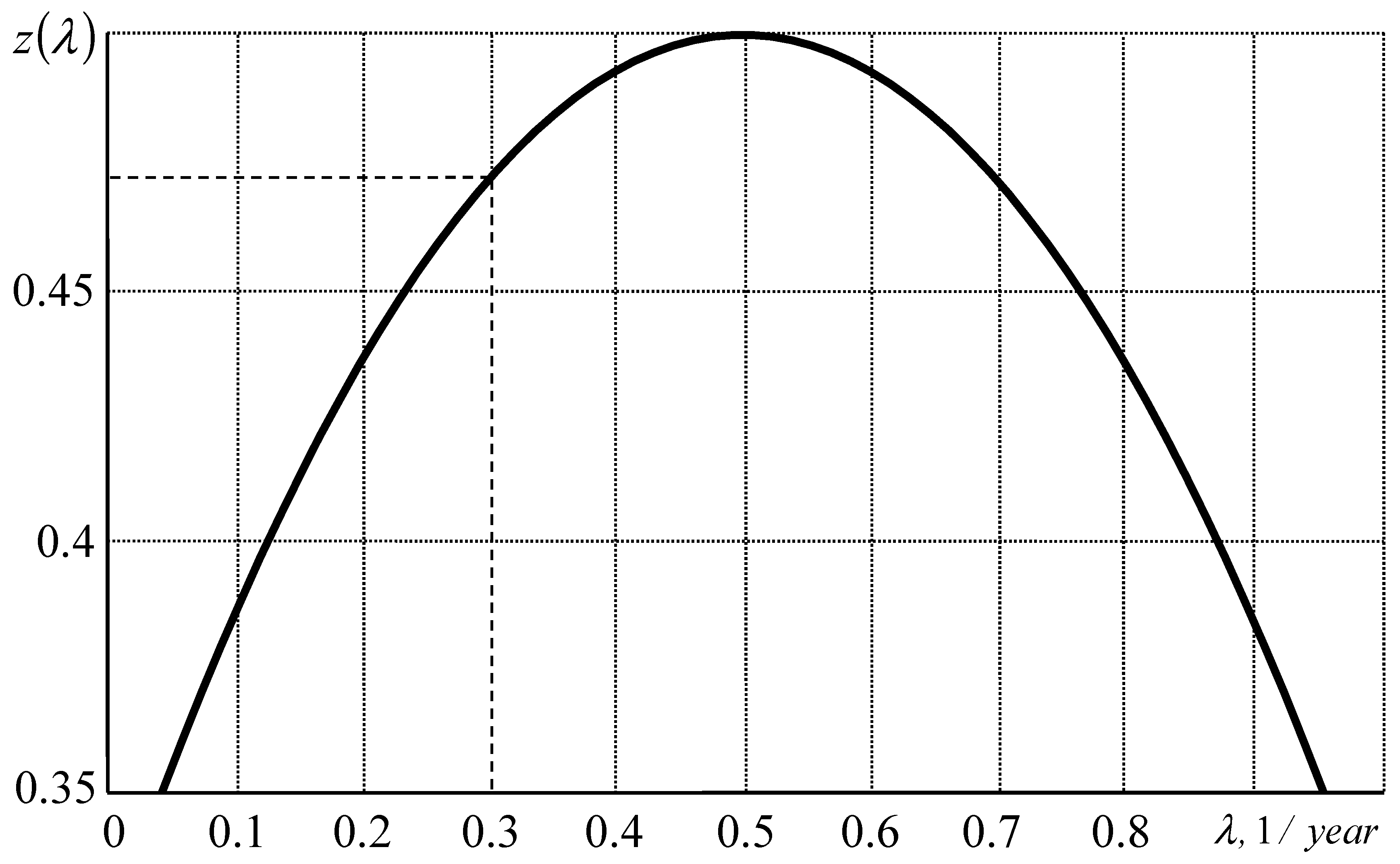
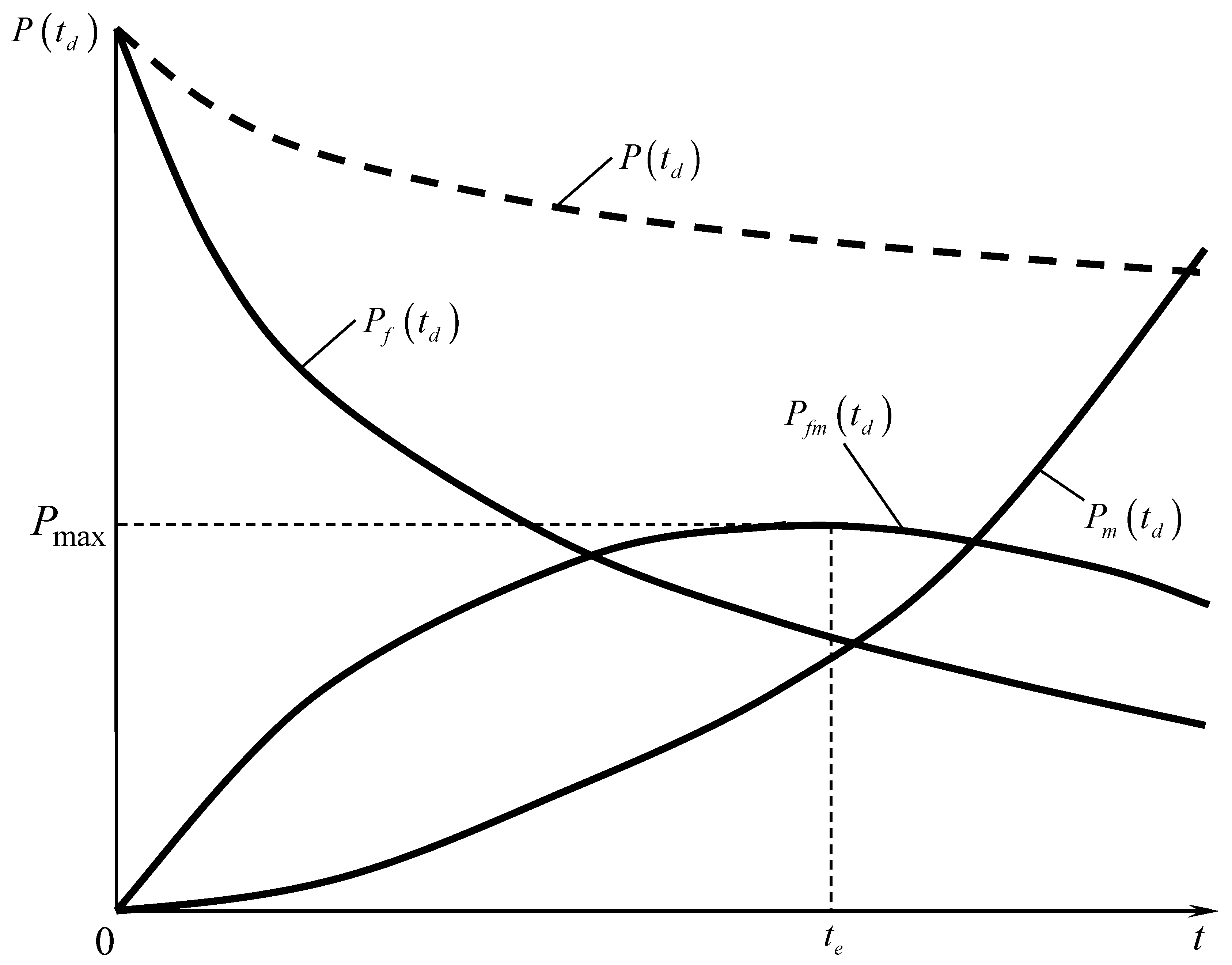
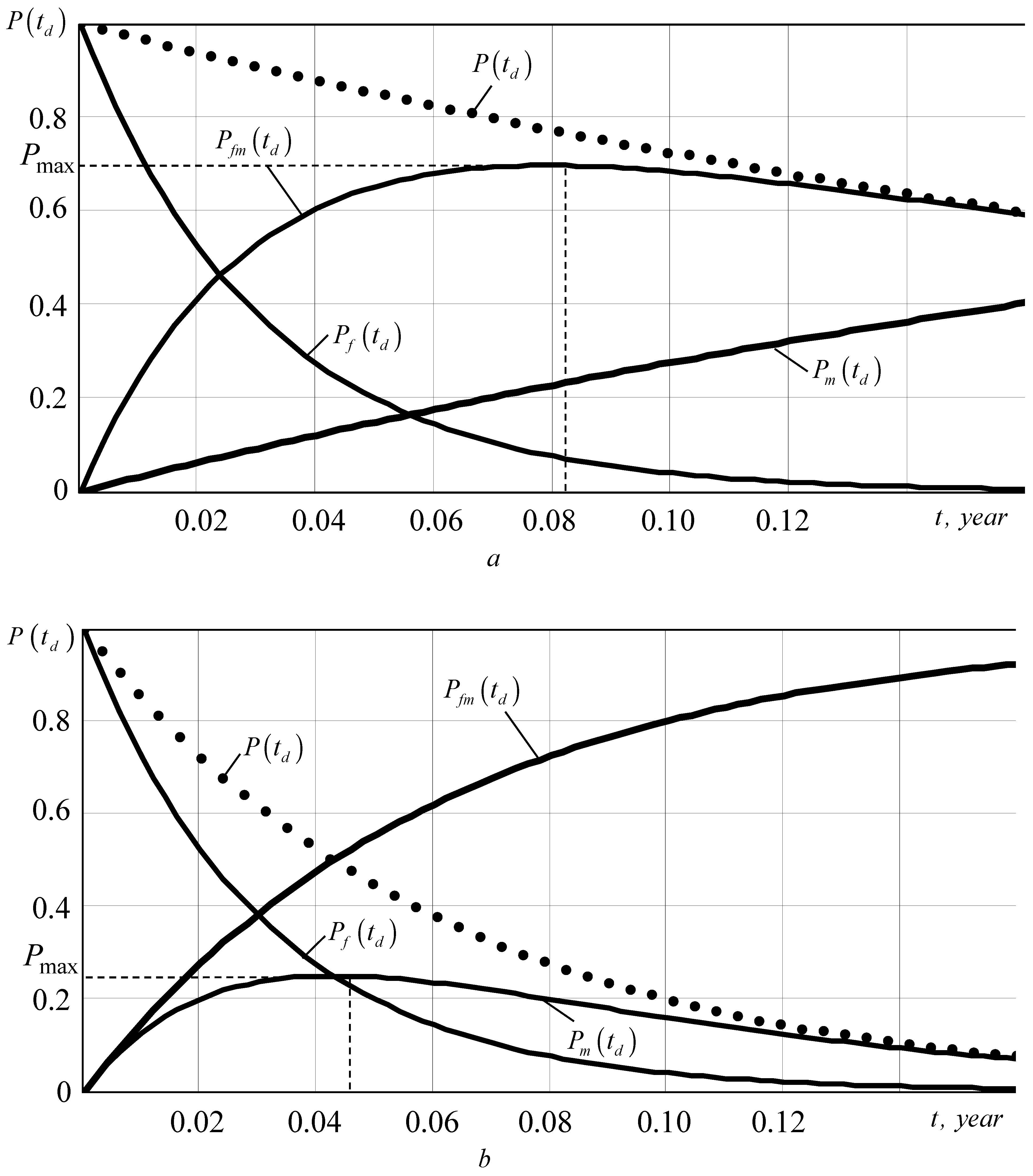
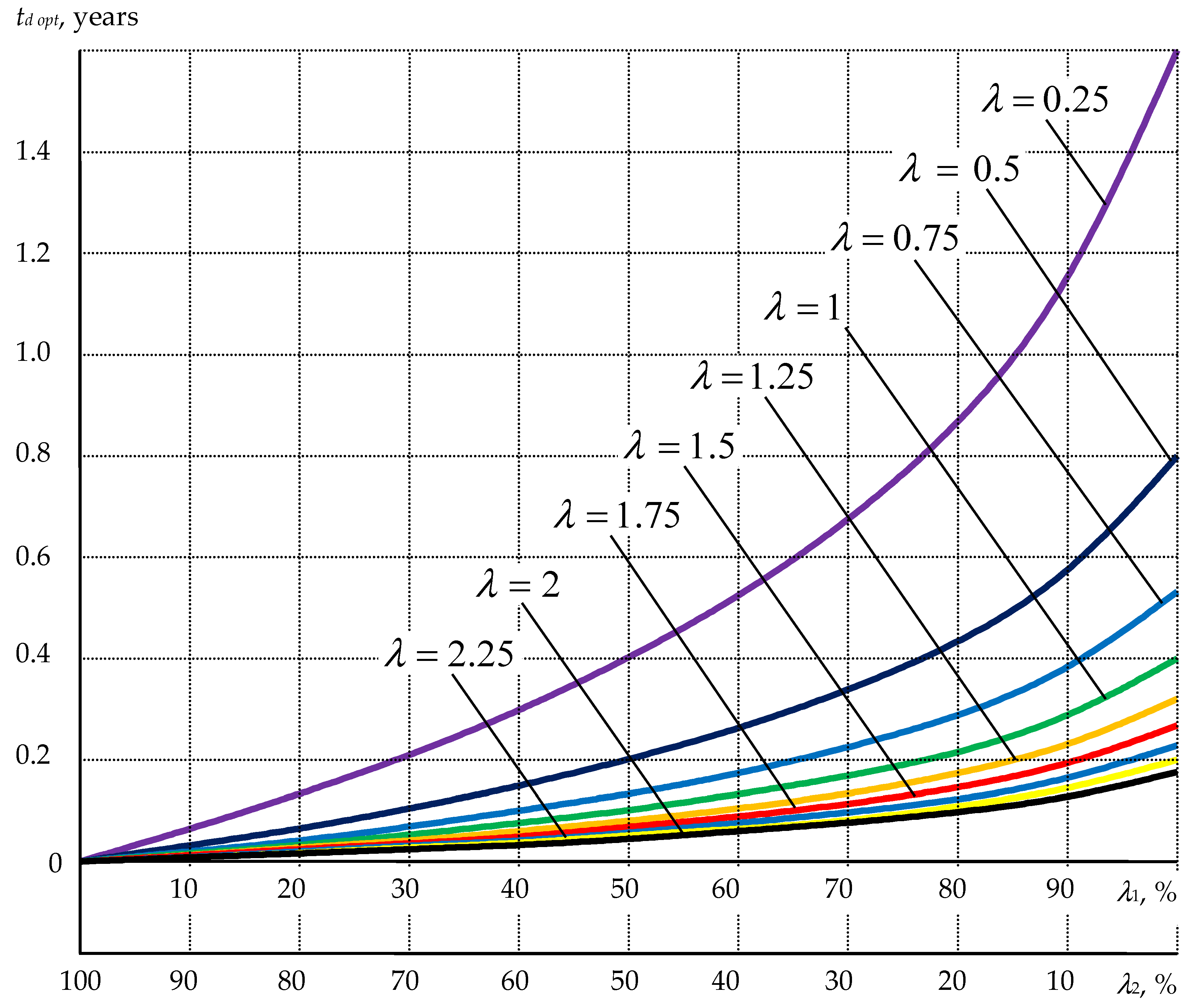
4. Influence of the Balance of Failures and Faults of Electrical Equipment on the Terms of Its Diagnosis

Electrical equipment of a trolleybus can be faulty, defective and failed (Figure 1). The average intensity of fault occurrence λ₁ and failure occurrence λ₂ are related to the average times T₁ and T₂, respectively, by the expressions

$${\lambda }_1=\frac{1}{T_1}, {\lambda }_2=\frac{1}{T_2}.$$

(16)

During the analysis we used the statistical material, which characterizes the intensity of failures and malfunctions. The occurrence of malfunctions was taken as a delay in the release of the trolleybus. Further on, this assumption means that the reliability of fault detection during preventive maintenance is not required above the one accepted for the monitoring of the vehicles leaving the line. The cases of returns from the line and cases of downtime on the line were taken as failures. Then, the time T₂—the time of transition of the fault to failure, will be determined as follows

$$T_2=\frac{\mathit{number} \mathit{of} \mathit{working} \mathit{days}}{\mathit{number} \mathit{of} \mathit{failures}}-\frac{\mathit{number} \mathit{of} \mathit{working} \mathit{days}}{\mathit{number} \mathit{of} \mathit{failures}+\mathit{number} \mathit{of} malfunction}.$$

(17)

If the intensity of failures and faults (which was taken as λ₁, since every failure is preceded by a fault) is much higher than the intensity of failures λ₂, then we can assume that the statistics of faults weakly affects the statistics of failures, that is, the correlation between T₁ and T₂ is weak. Otherwise, the correlation between T₁ and T₂ is large and must be taken into account. The characteristic of the relationship is the ratio

$$\rho =\frac{{\lambda }_1}{{\lambda }_2}.$$

(18)

With the exponential character, the reliability function P(t) point t_{d opt} is determined from Equation (18)

$$t_{d opt}=\frac{\mathit{ln}{\lambda }_1-\mathit{ln}{\lambda }_2}{{\lambda }_1-{\lambda }_2}=\frac{\varphi \left(\rho \right)}{{\lambda }_2},$$

(19)

where φ(ρ) is a tabulated function [36]. Expression (19) in the presence of a linear relationship between T₁ and T₂ (ρ < 2) according to (18) can be refined by replacing the function

$${\varphi }_1\left(\rho \right)=\frac{\left(\rho +1\right)\cdot \ln \left(\rho +1\right)}{{\rho }^2}.$$

(20)

Using the above expressions (16)–(20) according to the statistical data, the calculation of the optimal inter-diagnostic period for each month of the year for the trolleybus TED was determined (

Table 4. Calculation of trolleybus traction motor inter-diagnostic periods.

Month	td opt, Days	td opt max, Days	td opt min, Days
January	8.1	8.9	7.5
February	8.5	9.3	7.9
March	6.1	6.7	5.6
April	5.1	5.6	4.7
May	5.1	5.7	4.7
June	6.7	7.3	6.1
July	11.0	12.0	10.0
August	7.3	8.0	6.7
September	9.0	10.5	8.8
October	9.3	10.0	8.5
November	9.8	9.8	8.7
December	9.7	9.3	8.9

). In the calculation, the relationship between the times T₁ and T₂ was considered weak. The confidence approximation interval at confidence probability α = 0.9 has boundaries from +9 to −8% of the optimum.

In fact, there is a connection between the times T₁ and T₂. However, in the case of such a complicated electrical complex as a trolleybus EE, in general, this relationship can be neglected in order to simplify the calculations. If this relationship is taken into account, the inter-protective period according to Table 3 will be somewhat longer. For example, if the relationship between T₁ and T₂ is considered linear, then t_{d opt} increases by 5–10%.

Thus, as follows from Table 3, if the repair work, regular maintenance work and the level of control of the machines when they go on the line remain unchanged, then the methodology adopted by [27] for determining the optimal timing of preventive maintenance (diagnosis and partial adjustment) of electrical equipment leads to an increase relative to the existing timing.

The effect of increasing the efficiency of EE monitoring before going to the line, i.e., the effect of fault detection efficiency, was estimated as follows. Let us say, for example, that in August when the line was released there were not 63 faults, but 76 (an increase of 20%). The number of faults on the line will correspondingly be 13 less.

According to the adopted method of optimizing the time t_d, the new optimal time t_d will be 8.5 days instead of 7.3 days, that is, there is an opportunity to increase the inter-diagnostic period by 20%.

The given distributions and calculations allow us to make conclusions about useful diagnostic terms. The diagnostics terms differ from the regulation ones; this is explained by the fact that the calculation of diagnostics terms (Table 3) is aimed at optimizing the inter-diagnostic period at a given intensity of failures (or flow of failures, which is the same at λ(t) = const), but not at achieving the maximum given level of reliability of trolleybus electrical equipment.

The paper obtained the dependence between the optimal diagnostic time t_{d opt} on the intensity of failures of electrical equipment λ₁ and the intensity of its failures λ₂. According to (19)

$$t_{d opt}=\frac{\mathit{ln}{\lambda }_1-\mathit{ln}{\lambda }_2}{{\lambda }_1-{\lambda }_2}=\frac{\mathit{ln}\left(\frac{{\lambda }_1}{{\lambda }_2}\right)}{{\lambda }_2\cdot \left(\frac{{\lambda }_1}{{\lambda }_2}-1\right)}.$$

(21)

Denoting $z=\frac{{\lambda }_1}{{\lambda }_1+{\lambda }_2}$, we obtain

$$t_{d opt}=\frac{2\cdot z-1}{\mathit{ln}\left(\frac{z}{1-z}\right)\cdot \lambda },$$

(22)

where λ = λ₁ + λ₂.

Obviously, at λ = 0.5 the function z(λ) has uncertainty. Using the theory of limits to find uncertain values of functions [37], we obtain a value of the function equal to 0.5 at λ = 0.5.

The graph in Figure 11 shows the dependence between the parameter z and the failure rate λ for determining the optimal diagnostic time for trolleybus electrical equipment. So, having λ = 1/3, we get z = 0.481. That is, at failure of electrical equipment, equal to the third part of the total number of its failures (λ₁ = 0.3λ), (λ₂ = 0.7λ), the optimal time of diagnostics of trolleybus electrical equipment will be defined as

$$t_{d opt}=\frac{0.481}{\lambda }.$$

(23)

Dependence z(λ) (Figure 11) also allows you to estimate the diagnostic time of electrical equipment in the case where only the total number of equipment failures is determined without differentiating these failures into soft failures (eliminated before operation) and hard failures (leading to line downtime and returns to the depot for unscheduled repairs) [38].

Let’s determine the optimal diagnostic time t_{d opt} using the laws of distribution of the probability of occurrence of a failure and failure in the interventional period [39,40,41,42].

The probability of failure (together with the failure) is determined by the expression depending on the inter-protective time

$$P_f=1-{\displaystyle \underset{0}{\overset{t_d}{\int }}{f}_1\left(\tau \right)\cdot d\tau },$$

(24)

where f₁(τ) is the probability density of occurrence of failure. The probability of occurrence of a failure during the inter-protective period is equal to

$$P_m={\displaystyle \underset{0}{\overset{t_d}{\int }}{f}_0\left(\tau \right)\cdot d\tau }.$$

(25)

Since the general state of the object corresponds to unit probability (ΣP = 1), the probability that a failure will occur before the next preventive maintenance, but no failure will occur (return from the line or idle time on the line) is defined as the difference

$$P_{fm}=1-P_f\left(t_d\right)-P_m\left(t_d\right).$$

(26)

The general view of the dependencies P_fm(t_d), P_f(t_d), P_m(t_d) for trolleybus EE under the exponential law of reliability change is shown in Figure 12.

The function P_f(t_d) determines the probability that neither failures nor malfunctions will occur (sum of neither); P_m(t_d) is the probability of failure; 1 − P_f(t_d) − P_m(t_d) is the probability of malfunction; 1 − P_f(t_d) is the probability of both failure and malfunction (sum of both); P(t_d).

The function P_f (t_d) is decreasing and together with P_fm(t_d) form the reliability function, which was adopted earlier as an exponential law of reliability. The function P_m is non-decreasing. The intensity of failures of the object (the parameter of the flow of failures of the repaired object) will be minimal, if it is possible to use the maximum “resource of faulty operation” [43,44].

In this case, of course, the amount of works on preventive maintenance can increase, but relative to the failures per unit time will achieve a minimum, which for a long period will give a reduction in the total number of failures. If the quality of preventive work, despite some increase in the volume of work, will not change, then the inter-diagnostic period t_d, corresponding to the maximum, will be optimal. Both the decrease in t_d, relative to it, and the increase will give the increase in the total number of failures for the longer period [45,46,47].

Depending on the nature of the reliability function P(t), the point t_{d opt} is defined as the maximum of the function P_fm(t_d) (Figure 12).

Thus, the optimum time between adjustments of the node is

$$t_{d opt}=\frac{P_{\mathit{max}}}{\lambda }.$$

(27)

Figure 13 shows the dependences P_fm(t_d), P_f(t_d), P_m(t_d) for determining the optimal time between adjustments of EE at λ = 0.647 and different fractions of faults in the sum of faults and failures.

It has been determined that depending on the number of failures detected during preventive inspection or repair, λ₁ is the optimum time between adjustments of the unit t_{d opt}, with t_{d opt} not depending on the intensity of failures λ, but only on the balance of failures λ₁ and failures λ₁.

Table 5. Calculation of optimal inter-diagnostic periods of trolleybus electrical equipment t_{d opt} with different balances of faults and failures.

Malfunction λ1, %		0	10	20	30	40	50	60	70	80	90	100
Failures λ2, %		100	90	80	70	60	50	40	30	20	10	0
λ = 0.05	Pmax, r.u.	0	0.04	0.08	0.13	0.19	0.25	0.33	0.42	0.53	0.70	1
	td opt, years	0	0.33	0.64	0.98	1.11	1.3	1.72	2.31	3.01	3.9	8
λ = 0.25	Pmax, r.u.	0	0.04	0.08	0.13	0.19	0.25	0.33	0.42	0.53	0.70	1
	td opt, years	0	0.16	0.33	0.52	0.74	1	1.30	1.67	2.14	2.79	4
λ = 0.5	Pmax, r.u.	0	0.04	0.08	0.13	0.19	0.25	0.33	0.42	0.53	0.70	1
	td opt, years	0	0.08	0.16	0.26	0.37	0.5	0.65	0.84	1.07	1.39	2
λ = 0.75	Pmax, r.u.	0	0.04	0.08	0.13	0.19	0.25	0.33	0.42	0.53	0.70	1
	td opt, years	0	0.05	0.1	0.17	0.25	0.33	0.43	0.56	0.71	0.93	1.33
λ = 1	Pmax, r.u.	0	0.04	0.08	0.13	0.19	0.25	0.33	0.42	0.53	0.70	1
	td opt, years	0	0.04	0.08	0.13	0.19	0.25	0.33	0.42	0.53	0.70	1
λ = 1.25	Pmax, r.u.	0	0.04	0.08	0.13	0.19	0.25	0.33	0.42	0.53	0.70	1
	td opt, years	0	0.03	0.07	0.10	0.15	0.20	0.26	0.33	0.43	0.56	0.8
λ = 1.5	Pmax, r.u.	0	0.04	0.08	0.13	0.19	0.25	0.33	0.42	0.53	0.70	1
	td opt, years	0	0.03	0.06	0.09	0.12	0.17	0.22	0.28	0.36	0.47	0.67
λ = 1.75	Pmax, r.u.	0	0.04	0.08	0.13	0.19	0.25	0.33	0.42	0.53	0.70	1
	td opt, years	0	0.02	0.05	0.08	0.10	0.14	0.19	0.24	0.30	0.40	0.57
λ = 2	Pmax, r.u.	0	0.04	0.08	0.13	0.19	0.25	0.33	0.42	0.53	0.70	1
	td opt, years	0	0.02	0.04	0.07	0.09	0.13	0.16	0.20	0.27	0.35	0.5
λ = 2.25	Pmax, r.u.	0	0.04	0.08	0.13	0.19	0.25	0.33	0.42	0.53	0.70	1
	td opt, years	0	0.02	0.04	0.06	0.08	0.11	0.15	0.19	0.24	0.31	0.44

shows the calculation of optimal inter-diagnostic periods of trolleybus electrical equipment t_{d opt} at different balance of faults and failures and intensity of failures λ, 1/year. Plots of dependences t_{d opt}(λ₁) and t_{d opt}(λ₂) for trolleybus electrical equipment failure intensity range λ = [0.25 … 2.25] are shown in Figure 14.

It is easy to see that with the increase in faults (defects, minor failures, eliminated directly at the release of rolling stock) in relation to failures (severe forms of failure, leading to the derailment of the rolling stock from the line) diagnostic time increases and vice versa [48,49,50,51,52].

Thus, having detailed statistical information on EE failures (including information about the significance of the failure, the degree of consequence of the failure for further operation of the rolling stock), you can find the optimal value of both the preventive period and the diagnostic period for each type of trolleybus EE [53].

It should be noted that according to the proposed methodology it is possible to determine the preventive maintenance period and diagnostic terms both for the EE unit as a whole and for its individual element (unit, node), which contributes to the optimization of diagnostic work on labor intensity and cost-effectiveness.

The results of the calculation of t_{d opt} in the most typical case, when the faults detected during the preventive inspection or repair are λ₁ = 30%, and the failures are λ₂ = 70% are presented in Table 1 for each type of EE.

The quality of existing diagnostics is indirectly represented by the share of rolling units returned from the line of the total number of defective machines. The higher this share, the more imperfect are the existing methods of initial defect detection. The data on the return rate k_returns are presented in Table 1. According to the given evaluation, the following elements are characterized as fault-tolerant elements: starting and shunt resistance, insulation resistance of the trolleybus (leakage current), auxiliary motor of the door drive, accumulator, traction motor, relay-regulator, motor-compressor. The coefficient k_returns in addition to diagnostic imperfection characterizes the degree of influence of line conditions on the object (Figure 13) and the degree of refinement of the trolleybus EE design.

Due to the analysis performed, a number of EE units were identified for which, first of all, it is necessary to ensure quick and correct fault diagnosis in order to perform as few breakdowns disturbing the running-in process as possible during repair. In order to reduce the effect of running-in, the following units should be selected from the list in Table 1: control circuit, controller and reverser, traction motor, contactor, auxiliary motor.

In this paper we managed to identify failures that do not lead to failures, and they can be promptly eliminated, and failures of electrical complexes that lead to irregular removal of electric rolling stock from the line and their repair at a time when the electric bus should have been on the line. We have highlighted that inter-repair failures are the most undesirable equipment failures. Additionally, the presented model makes it possible to analyze the fact that when the equipment is restored during the maintenance of the system units, the recovery of the whole system is not 100%, and each subsequent restoration of the system worsens its reliability indicators. Here the parameter of the resource recovery factor is used. By the coefficient of restoration of the resource of an element is understood the probability of how much the restoration of the resource correlates with a new element that has a probability of failure-free operation (Figure 2). Thus, it allows the estimation of the time of the trolleybus EE diagnostics more precisely and allows the refining of it in comparison with the existing one. The authors made proposals to change the preventive maintenance regulations, the main task of which became the detection of a malfunction that can lead to total failure. In this case, preventive maintenance turns into combined preventive maintenance for the applied rolling stock units.

Since the proposed method is based on the theory of probability and mathematical statistics, the limitations of the presented method can be considered to be the accepted independence of failures of electrical equipment elements from each other. At the same time, taking into account that in trolleybuses and electric buses there are hundreds of systems with the total number of subsystems, units, elements and parts exceeding ten thousand, it is very important to take into account the mutual influence of these components on each other when determining the reliability of the entire system (Figure 3). For example, the authors have experimentally established that failures of mechanical equipment of electric buses (transmission, gearbox, cardan shafts, etc.) can cause malfunctions and failures of the traction motor. Taking into account these mutual influences not only qualitatively, but also quantitatively by means of mathematical analysis can improve the accuracy of determining and predicting the reliability of electrical equipment of modern trolleybuses and electric buses.

5. Conclusions

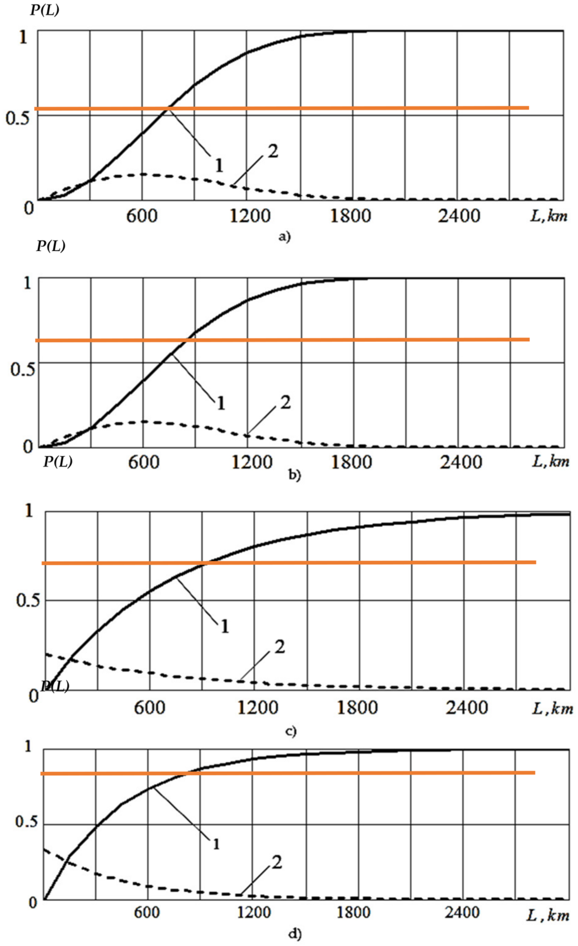
• As a result of processing statistical information on failures, it was found that for trolleybus electrical equipment after a number of repair actions, the maximum failure density occurs at lower mileage, and the probability of failure-free operation can vary depending on the degree of wear of the equipment, i.e., on the number of previous failures. In addition, Gauss’s law is valid for brand new electrical equipment. In all other cases, Rayleigh’s uniform and exponential law is more valid. This analysis allows us to say that the recovery of technical reliability of trolleybus and electric bus subsystems is not complete and it is necessary to take into account the recovery factor of the whole system, which will be the subject of future research.
• The dependence of switching equipment run-in on time has been clarified, which served as a prerequisite for specifying the inter-repair period for each type of trolleybus electrical equipment. The method of adjustment of the inter-repair time for the electrical equipment of trolleybuses is proposed.
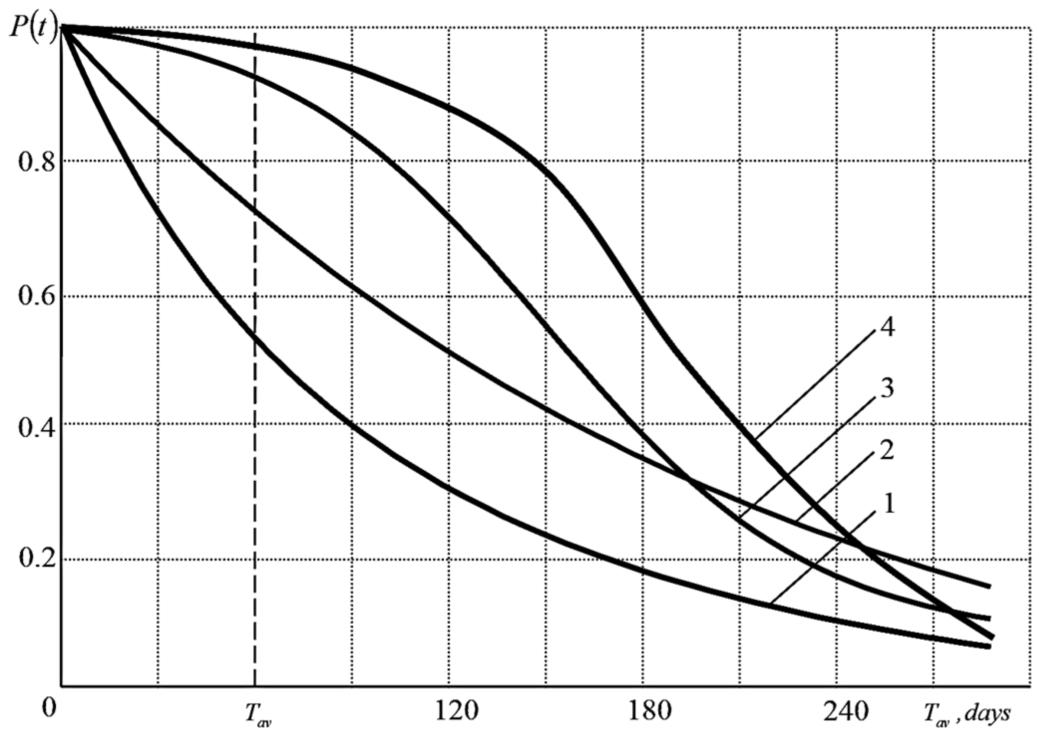
• It is theoretically substantiated and experimentally confirmed that the reliability of electrical equipment of trolleybuses in operation changes according to the exponential law. It has been established that the real average diagnostics terms regulated by instructions are not optimal in most cases and differ several times from those defined in the work. Thus, it is necessary to switch from the planned preventive repair system to the system of repairs according to need (according to the current technical condition).
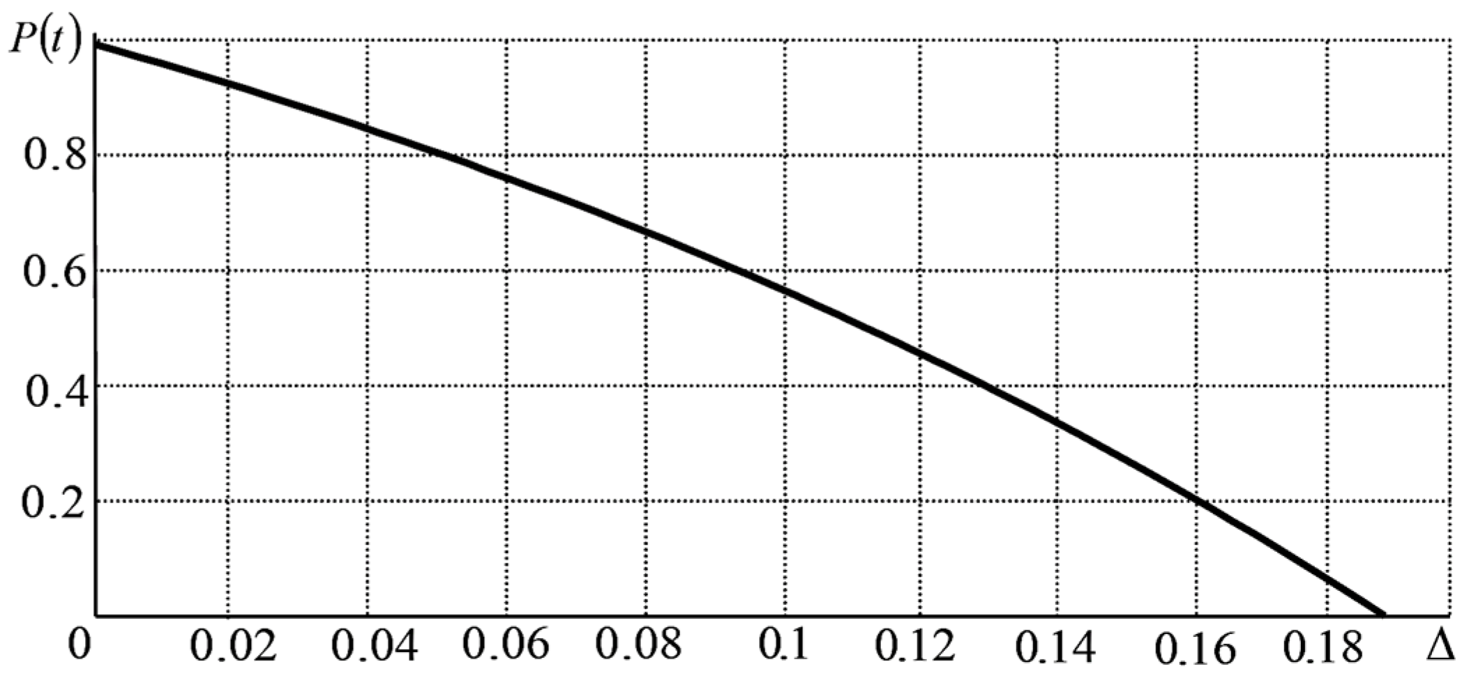
• On the basis of reliability theory, probability theory and mathematical statistics, numerical methods of nonlinear and transcendental equations solution, the terms of diagnostics t_d depending on failure intensity λ(t) and given probability of equipment no-failure operation P(t) are determined. The inverse problem of determining the current reliability of electrical engineering systems depending on the diagnostic time t_d and the failure rate λ (t) is also solved.
• The effect of fault balance λ₁ and failures λ₂ in the sum of faults and failures λ on the optimal time between adjustments t_{d opt} of electrical equipment is investigated. It is concluded that t_{d opt} depends on the balance of faults λ₁ and failures λ₂. The calculation of optimum between-diagnostic periods of t trolleybus electrical equipment t_{d opt} with different balance of failures λ₁ and failures λ₂ was achieved.

References

1. Campbell, R.J. CRS Report for Congress: Weather-Related Power Outages and Electric System Resiliency. 2012. Available online: https://sgp.fas.org/crs/misc/R42696.pdf (accessed on 3 December 2021).
2. Wang, Y.; Chen, C.; Wang, J.; Baldick, R. Research on Resilience of Power Systems under Natural Disasters—A Review. IEEE Trans. Power Syst. 2016, 31, 1604–1613. [Google Scholar] [CrossRef]
3. Martyushev, N.V.; Malozyomov, B.V.; Sorokova, S.N.; Efremenkov, E.A.; Qi, M. Mathematical Modeling the Performance of an Electric Vehicle Considering Various Driving Cycles. Mathematics 2023, 11, 2586. [Google Scholar] [CrossRef]
4. Ehsani, M.; Wang, F.-Y.; Brosch, G.L. (Eds.) Transportation Technologies for Sustainability; Springer: New York, NY, USA, 2013. [Google Scholar]
5. Chan, C.C.; Bouscayrol, A.; Chen, K. Electric, Hybrid, and Fuel-Cell Vehicles: Architectures and Modeling. IEEE Trans. Veh. Technol. 2010, 59, 589–598. [Google Scholar] [CrossRef]
6. Colvile, R.N.; Hutchinson, E.J.; Mindell, J.S.; Warren, R.F. The transport sector as a source of air pollution. Atmos. Environ. 2001, 35, 1537–1565. [Google Scholar] [CrossRef] [Green Version]
7. Wang, Q.; Wu, Z. Structural System Reliability Analysis Based on Improved Explicit Connectivity BNs. KSCE J. Civ. Eng. 2018, 22, 916–927. [Google Scholar] [CrossRef]
8. Malozyomov, B.V.; Martyushev, N.V.; Sorokova, S.N.; Efremenkov, E.A.; Qi, M. Mathematical Modeling of Mechanical Forces and Power Balance in Electromechanical Energy Converter. Mathematics 2023, 11, 2394. [Google Scholar] [CrossRef]
9. Xia, Q.; Wang, Z.; Ren, Y.; Sun, B.; Yang, D.; Feng, Q. A reliability design method for a lithium-ion battery pack considering the thermal disequilibrium in electric vehicles. J. Power Sources 2018, 386, 10–20. [Google Scholar] [CrossRef]
10. Mingers, J. A critique of statistical modelling from a critical realist perspective. In Proceedings of the 11th European Conference on Information Systems, ECIS 2003, Naples, Italy, 16–21 June 2003; pp. 1277–1288. [Google Scholar]
11. Wang, Q.A.; Zhang, C.; Ma, Z.G.; Ni, Y.Q. Modelling and forecasting of SHM strain measurement for a large-scale suspension bridge during typhoon events using variational heteroscedastic Gaussian process. Eng. Struct. 2022, 251, 113554. [Google Scholar] [CrossRef]
12. Balagurusamy, E. Reliability Engineering, First. P-24, Green Park Extension; McGraw Hill Education (India) Private Limited: New Delhi, India, 2002. [Google Scholar]
13. Oluwasuji, O.I.; Malik, O.; Zhang, J.; Ramchurn, S.D. Solving the fair electric load shedding problem in developing countries. Auton. Agents Multi-Agent Syst. 2019, 34, 12. [Google Scholar] [CrossRef] [Green Version]
14. Malozyomov, B.V.; Golik, V.I.; Brigida, V.; Kukartsev, V.V.; Tynchenko, Y.A.; Boyko, A.A.; Tynchenko, S.V. Substantiation of Drilling Parameters for Undermined Drainage Boreholes for Increasing Methane Production from Unconventional Coal-Gas Collectors. Energies 2023, 16, 4276. [Google Scholar] [CrossRef]
15. Lacey, G.; Putrus, G.; Bentley, E. Smart EV charging schedules: Supporting the grid and protecting battery life. IET Electr. Syst. Transp. 2017, 7, 84–91. [Google Scholar] [CrossRef]
16. Aggarwal, K.K. Maintainability and Availability, Topics in Safety Reliability and Quality; Springer: Dordrecht, The Netherlands, 1993. [Google Scholar]
17. Shu, X.; Guo, Y.; Yang, W.; Wei, K.; Zhu, Y.; Zou, H. A Detailed Reliability Study of the Motor System in Pure Electric Vans by the Approach of Fault Tree Analysis. IEEE Access 2020, 8, 5295–5307. [Google Scholar] [CrossRef]
18. Shchurov, N.I.; Myatezh, S.V.; Malozyomov, B.V.; Shtang, A.A.; Martyushev, N.V.; Klyuev, R.V.; Dedov, S.I. Determination of Inactive Powers in a Single-Phase AC Network. Energies 2021, 14, 4814. [Google Scholar] [CrossRef]
19. Shchurov, N.I.; Dedov, S.I.; Malozyomov, B.V.; Shtang, A.A.; Martyushev, N.V.; Klyuev, R.V.; Andriashin, S.N. Degradation of Lithium-Ion Batteries in an Electric Transport Complex. Energies 2021, 14, 8072. [Google Scholar] [CrossRef]
20. Malozyomov, B.V.; Martyushev, N.V.; Kukartsev, V.A.; Kukartsev, V.V.; Tynchenko, S.V.; Klyuev, R.V.; Zagorodnii, N.A.; Tynchenko, Y.A. Study of Supercapacitors Built in the Start-Up System of the Main Diesel Locomotive. Energies 2023, 16, 3909. [Google Scholar] [CrossRef]
21. Xia, Q.; Wang, Z.; Ren, Y.; Tao, L.; Lu, C.; Tian, J.; Hu, D.; Wang, Y.; Su, Y.; Chong, J.; et al. A modified reliability model for lithium-ion battery packs based on the stochastic capacity degradation and dynamic response impedance. J. Power Sources 2019, 423, 40–51. [Google Scholar] [CrossRef]
22. Isametova, M.E.; Nussipali, R.; Martyushev, N.V.; Malozyomov, B.V.; Efremenkov, E.A.; Isametov, A. Mathematical Modeling of the Reliability of Polymer Composite Materials. Mathematics 2022, 10, 3978. [Google Scholar] [CrossRef]
23. Bolvashenkov, I.; Herzog, H.-G. Approach to predictive evaluation of the reliability of electric drive train based on a stochastic model. In Proceedings of the 2015 International Conference on Clean Electrical Power (ICCEP), Taormina, Italy, 16–18 June 2015; pp. 486–492. [Google Scholar]
24. Ammaiyappan, B.S.; Ramalingam, S. Reliability investigation of electric vehicles. Life Cycle Reliab. Saf. Eng. 2019, 8, 141–149. [Google Scholar] [CrossRef]
25. Alberta Utilities Commission. Waterton Battery Energy Storage System. 2021. Available online: https://efiling-webapi.auc.ab.ca/Document/Get/683303 (accessed on 3 December 2021).
26. Li, J.; Niu, D.; Wu, M.; Wang, Y.; Li, F.; Dong, H. Research on Battery Energy Storage as Backup Power in the Operation Optimization of a Regional Integrated Energy System. Energies 2018, 11, 2990. [Google Scholar] [CrossRef] [Green Version]
27. HSB. Maintaining Emergency and Standby Engine-Generator Sets. 2020. Available online: https://www.munichre.com/content/dam/munichre/global/content-pieces/documents/447-Recommended-Practice-for-Maintaining-Emergency-and-StandbyEngine-Generator-Sets.pdf/_jcr_content/renditions/original.media_file.download_attachment.file/447-RecommendedPractice-for-Maintainig-Emergency-and-Standby-Engine-Generator-Sets.pdf (accessed on 13 January 2022).
28. International Energy Agency. Global EV Outlook 2021 Overview; International Energy Agency: Paris, France, 2021.
29. Electric Vehicle Database Useable Battery Capacity of Fully Electric Vehicles Cheatsheet—EV Database. Available online: https://ev-database.org/cheatsheet/useable-battery-capacity-electric-car (accessed on 3 December 2021).
30. Salvatti, G.A.; Carati, E.G.; Cardoso, R.; da Costa, J.P.; Stein, C.M.D.O. Electric Vehicles Energy Management with V2G/G2V Multifactor Optimization of Smart Grids. Energies 2020, 13, 1191. [Google Scholar] [CrossRef] [Green Version]
31. Kasturi, K.; Nayak, C.K.; Nayak, M.R. Electric vehicles management enabling G2V and V2G in smart distribution system for maximizing profits using MOMVO. Int. Trans. Electr. Energy Syst. 2019, 29, e12013. [Google Scholar] [CrossRef]
32. Billinton, R.; Allan, R.N. Reliability Evaluation of Engineering Systems; Springer: Boston, MA, USA, 1992. [Google Scholar]
33. Malozyomov, B.V.; Kukartsev, V.V.; Martyushev, N.V.; Kondratiev, V.V.; Klyuev, R.V.; Karlina, A.I. Improvement of Hybrid Electrode Material Synthesis for Energy Accumulators Based on Carbon Nanotubes and Porous Structures. Micromachines 2023, 14, 1288. [Google Scholar] [CrossRef]
34. Malozyomov, B.V.; Martyushev, N.V.; Kukartsev, V.V.; Tynchenko, V.S.; Bukhtoyarov, V.V.; Wu, X.; Tyncheko, Y.A.; Kukartsev, V.A. Overview of Methods for Enhanced Oil Recovery from Conventional and Unconventional Reservoirs. Energies 2023, 16, 4907. [Google Scholar] [CrossRef]
35. Billinton, R.; Allan, R.N. Reliability Evaluation of Power Systems, 2nd ed.; Springer: Boston, MA, USA, 1996. [Google Scholar]
36. Martyushev, N.V.; Malozyomov, B.V.; Khalikov, I.H.; Kukartsev, V.A.; Kukartsev, V.V.; Tynchenko, V.S.; Tynchenko, Y.A.; Qi, M. Review of Methods for Improving the Energy Efficiency of Electrified Ground Transport by Optimizing Battery Consumption. Energies 2023, 16, 729. [Google Scholar] [CrossRef]
37. Li, X.; Tan, Y.; Liu, X.; Liao, Q.; Sun, B.; Cao, G.; Li, C.; Yang, X.; Wang, Z. A cost-benefit analysis of V2G electric vehicles supporting peak shaving in Shanghai. Electr. Power Syst. Res. 2020, 179, 106058. [Google Scholar] [CrossRef]
38. Yoo, Y.; Al-Shawesh, Y.; Tchagang, A. Coordinated control strategy and validation of vehicle-to-grid for frequency control. Energies 2021, 14, 2530. [Google Scholar] [CrossRef]
39. Haghi, H.V.; Qu, Z. A Kernel-Based Predictive Model of EV Capacity for Distributed Voltage Control and Demand Response. IEEE Trans. Smart Grid 2018, 9, 3180–3190. [Google Scholar] [CrossRef]
40. Agarwal, L.; Peng, W.; Goel, L. Using EV battery packs for vehicle-to-grid applications: An economic analysis. In Proceedings of the 2014 IEEE Innovative Smart Grid Technologies—Asia (ISGT ASIA), Kuala Lumpur, Malaysia, 20–23 May 2014; IEEE Computer Society: Piscataway Township, NJ, USA, 2014; pp. 663–668. [Google Scholar]
41. Kataoka, R.; Ogimoto, K.; Iwafune, Y. Marginal Value of Vehicle-to-Grid Ancillary Service in a Power System with Variable Renewable Energy Penetration and Grid Side Flexibility. Energies 2021, 14, 7577. [Google Scholar] [CrossRef]
42. Martyushev, N.V.; Malozyomov, B.V.; Sorokova, S.N.; Efremenkov, E.A.; Qi, M. Mathematical Modeling of the State of the Battery of Cargo Electric Vehicles. Mathematics 2023, 11, 536. [Google Scholar] [CrossRef]
43. Młyńczak, M.; Nowakowski, T.; Restel, F.; Werbin´ska-Wojciechowska, S. Problems of Reliability Analysis of Passenger Transportation Process. In Proceedings of the European Safety and Reliability Conference, Balkema, Leiden, The Netherlands, 2–4 October 2011; pp. 1433–1438. [Google Scholar]
44. Chakrabarti, S. The Demand for Reliable Transit Service: New Evidence Using Stop Level Data from the Los Angeles Metro Bus. System. J. Transp. Geogr. 2015, 48, 154–164. [Google Scholar] [CrossRef]
45. Fricker, J.D.; Whitford, R.K. Fundamentals of Transportation Engineering. A Multimodal Systems Approach; Pearson Education, Inc.: Upper Saddle River, NJ, USA, 2004; pp. 243–276. [Google Scholar]
46. Barabino, B.; Di Francesco, M.; Mozzoni, S. An Offline Framework for the Diagnosis of Time Reliability by Automatic Vehicle Location Data. IEEE Trans. Intell. Transp. Syst. 2016, 18, 583–594. [Google Scholar] [CrossRef]
47. Barabino, B.; Di Francesco, M.; Mozzoni, S. Time Reliability Measures in bus Transport Services from the Accurate use of Automatic Vehicle Location raw Data. Qual. Reliab. Eng. Int. 2017, 33, 969–978. [Google Scholar] [CrossRef]
48. Pulugurtha, S.S.; Imran, M.S. Modeling Basic Freeway Section Level-of-Service Based on Travel Time and Reliability. Case Stud. Transp. Policy 2020, 8, 127–134. [Google Scholar] [CrossRef]
49. Yang, W.; Xiang, Y.; Liu, J.; Gu, C. Agent-Based Modeling for Scale Evolution of Plug-in Electric Vehicles and Charging Demand. IEEE Trans. Power Syst. 2018, 33, 1915–1925. [Google Scholar] [CrossRef]
50. Nie, Y.; Chung, C.Y.; Xu, N.Z. System State Estimation Considering EV Penetration with Unknown Behavior Using Quasi-Newton Method. IEEE Trans. Power Syst. 2016, 31, 4605–4615. [Google Scholar] [CrossRef]
51. Gong, H.; Ionel, D.M. Optimization of aggregated EV power in residential communities with smart homes. In Proceedings of the 2020 IEEE Transportation Electrification Conference and Expo, ITEC 2020, Chicago, IL, USA, 23–26 June 2020; Institute of Electrical and Electronics Engineers Inc.: Piscataway, NJ, USA, 2020; pp. 779–782. [Google Scholar]
52. U.S. Department of Transportation. 2017 NHTS Data User Guide; Federal Highway Administration Office of Policy Information: Washington, DC, USA, 2018.
53. Zhang, P.; Qian, K.; Zhou, C.; Stewart, B.G.; Hepburn, D.M. A methodology for optimization of power systems demand due to electric vehicle charging load. IEEE Trans. Power Syst. 2012, 27, 1628–1636. [Google Scholar] [CrossRef]
Figure 1. Possible technical conditions of trolleybus electrical equipment during operation.
Mathematics 11 03260 g001
Figure 2. Distribution of failure rate—1 and density of distribution—2 of trolleybus traction motors: (a)—first failure; (b)—second failure; (c)—third failure; (d)—fourth failure.
Mathematics 11 03260 g002
Figure 3. Effect of different laws of distribution of trolleybus traction motor failure-free operation time on its reliability function: 1—exponential distribution law; 2—uniform distribution law; 3—Rayleigh distribution law; 4—normal distribution law.
Mathematics 11 03260 g003
Figure 4. Relative error Δ, allowed in the calculation of the reliability function.
Mathematics 11 03260 g004
Figure 5. Variation of failure rate of trolleybus electrical systems over a long period of operation: I—period of running-in, II—long period of operation; III—period before overhaul.
Mathematics 11 03260 g005
Figure 6. Change in object reliability in the system with periodic diagnostics and recovery to P(t) = 1: 1, 2, 3, 3, 4, 5 and are groups of homogeneous EE objects.
Mathematics 11 03260 g006
Figure 7. Graphical determination of the time between failures T with the known average annual reliability P and the period of diagnosis td.
Mathematics 11 03260 g007
Figure 8. Dependence of reliability for one year P ¯ a v and MTBF T at: 1—td = 3.5 days, 2—td = 7 days, 3—td = 14 days, 4—td = 28 days, 5—td = 56 days, 6—td = 112 days, 7—td = 224 days.
Mathematics 11 03260 g008
Figure 9. A three-dimensional surface ( P ¯ a v  , T, td) to determine T given td and P ¯ a v .
Mathematics 11 03260 g009
Figure 10. Dependence between failure rate λ and running-in time Trunning of trolleybus electrical switching equipment.
Mathematics 11 03260 g010
Figure 11. Dependence for determining the optimal diagnostic time of trolleybus electrical equipment between the parameter z and the failure rate λ.
Mathematics 11 03260 g011
Figure 12. General view of dependencies Pfm(td), Pf(td), Pm(td) for trolleybus electrical equipment.
Mathematics 11 03260 g012
Figure 13. Determination of the optimum period of inter-regulated operation of electrical equipment: (a)—at λ = 0.647 and 10% of faults in the sum of faults and failures; (b)—at λ = 0.647 and 50% of faults in the sum of faults and failures.
Mathematics 11 03260 g013
Figure 14. Calculation of optimal inter-diagnostic periods of t trolleybus electrical equipment td opt with different balances of faults λ1 and failures λ2.
Mathematics 11 03260 g014