1. Introduction
Bayesian analysis is a statistical approach that incorporates prior knowledge or beliefs with observed data to make probabilistic inferences and update our knowledge. It is named after the Reverend Thomas Bayes, an 18th-century British statistician, and theologian who developed the foundational principles of this method [
1].
In Bayesian analysis, the main focus is on estimating and updating the posterior probability distribution of parameters of interest, given the observed data and any prior information. This is done using Bayes’ theorem, which mathematically expresses the relationship between the prior probability, likelihood, and posterior probability. The prior probability represents our initial beliefs about the parameters, and the likelihood quantifies the compatibility between the observed data and the parameter values. By combining these elements, Bayesian analysis provides a coherent framework for inference [
1,
2].
One of the key advantages of Bayesian analysis is its ability to incorporate prior knowledge. This is particularly useful when there is limited data available or when expert opinions and historical information are valuable in making predictions or decisions. The use of prior information allows for a more nuanced and flexible analysis, accommodating subjective judgments and external evidence [
3,
4].
Bayesian analysis finds applications in a wide range of fields, including but not limited to:
- (1)
Medicine and Healthcare: Bayesian methods are employed in clinical trials, diagnostic tests, epidemiology, and personalized medicine to quantify uncertainty and make informed decisions.
- (2)
Finance and Economics: Bayesian analysis is used in risk assessment, portfolio optimization, forecasting, and economic modeling to account for uncertainty and update beliefs.
- (3)
Engineering: Bayesian techniques are applied in reliability analysis, optimization, and decision-making under uncertainty in various engineering domains.
- (4)
Machine Learning and Artificial Intelligence: Bayesian inference is used in probabilistic modeling, Bayesian networks, and Bayesian optimization to reason under uncertainty and provide robust predictions.
- (5)
Environmental Science: Bayesian analysis is utilized in environmental modeling, ecological studies, and climate change research to integrate diverse data sources and quantify uncertainty in predictions [
5].
In social and behavioral sciences, Bayesian data analysis has been more frequently used since software packages popular among social scientists supported model fitting for Bayesian models and Markov chain Monte Carlo simulations (MCMC). These developments are facilitated by the availability of tutorials, software programs, and introductory textbooks on practical analytic skills [
6,
7].
1.1. Bayesian Latent Variable Modeling
Bayesian latent variable modeling refers to a class of statistical modeling techniques that involve unobserved or latent variables. Latent variables are variables that are not directly measured or observed but are inferred based on observed data. Bayesian methods are particularly well-suited for latent variable modeling because they allow for the incorporation of prior beliefs and uncertainty in estimating the latent variables and their relationships with the observed variables [
1,
8,
9].
In Bayesian latent variable modeling, the goal is to estimate the values of the latent variables and their associated parameters, given the observed data and any prior knowledge. This is typically done by specifying a probabilistic model that describes the relationships between the latent variables and the observed variables. The model parameters are then estimated using Bayesian inference, which involves updating the prior beliefs to obtain the posterior distribution of the parameters given the observed data [
9].
Bayesian latent variable modeling has wide-ranging applications in various fields, including psychology, social sciences, econometrics, and machine learning. It allows researchers to capture and analyze complex relationships, account for measurement errors, handle missing data, and make predictions or inferences about the latent variables [
10,
11].
1.2. Bayesian Factor Analysis
In factor analysis, the Bayesian method is used to uncover latent variables or factors that underlie a set of observed variables. It combines the principles of factor analysis, which aims to identify common patterns or underlying dimensions in observed data, with Bayesian inference, which allows for the incorporation of prior beliefs and uncertainty in parameter estimation [
8,
10,
12].
In Bayesian factor analysis, the goal is to estimate the factor loadings, which represent the relationships between the latent factors and the observed variables, and the factor scores, which indicate the values of the latent factors for each individual. The method assumes that the observed variables are linearly related to the latent factors and that the observed variables are influenced by both specific (unique) factors and common factors shared across variables [
12,
13].
The Bayesian approach to factor analysis allows for the incorporation of prior information about the factor loadings and the factor scores. It also provides posterior distributions for the estimated parameters, which reflect both the observed data and the prior beliefs. This posterior distribution can be used to make inferences about the latent factors and their relationships with the observed variables [
12,
13,
14]
With factor models, Bayes estimation outperformed the mean- and variance-adjusted weighted least squares procedure with ordinal data [
15,
16]. This method incorporates prior information, thus increasing the accuracy of parameter estimates and reducing the number of Heywood solutions [
17,
18,
19].
1.3. Bayesian Latent Class Analysis
Bayesian latent class analysis (BLCA) is a statistical method used to identify unobserved subgroups or latent classes within a population based on observed categorical variables [
20]. It combines the principles of latent class analysis (LCA), which seeks to identify homogeneous subgroups within a population, with Bayesian inference techniques, which allow for the incorporation of prior beliefs and uncertainty in parameter estimation [
12,
20,
21].
In BLCA, the goal is to estimate the latent class membership probabilities and the conditional response probabilities for each observed categorical variable given the latent class membership. The latent class membership probabilities indicate the likelihood of each individual belonging to each latent class, while the conditional response probabilities describe the probability of observing each response category for each variable within each latent class [
20].
The Bayesian approach to latent class analysis allows for the integration of prior information about the latent class membership probabilities and the conditional response probabilities. It also provides posterior distributions for the estimated parameters, which reflect both the observed data and the prior beliefs. This posterior distribution can be used to make inferences about the latent classes and their relationships with the observed categorical variables [
20,
21,
22,
23]. While several studies investigated the effectiveness of the Bayesian method in factor analysis [
17,
18,
19], few studies examined this estimation procedure’s performance with latent class models.
Specifically, the classification precision of BLCA is an area that has received limited research attention. Despite the growing popularity of Bayesian methods in other areas of statistics, there has been a dearth of studies specifically examining the classification precision of BLCA.
Compared to traditional frequentist approaches, BLCA offers several advantages, such as the ability to incorporate prior information, handle missing data more effectively, and provide uncertainty estimates through posterior distributions. However, the specific performance of BLCA in terms of classification precision, as measured by metrics, such as entropy and average latent class probabilities, remains relatively unexplored.
The lack of research in this area can be attributed to various factors. First, BLCA involves complex modeling and estimation procedures, which require specialized knowledge and computational resources. This complexity may have deterred researchers from exploring the classification precision of BLCA in depth. Second, the focus of previous studies on LCA has predominantly been on model selection, identifying the appropriate number of latent classes, and examining the substantive interpretation of latent classes rather than evaluating classification precision. As a result, the evaluation of classification precision has often taken a backseat. Third, the availability of user-friendly software and computational tools for BLCA has been relatively limited compared to frequentist counterparts. This may have hindered researchers from conducting comprehensive studies on classification precision using Bayesian approaches.
Given the potential advantages of BLCA and the importance of classification precision in understanding latent class membership, there is a need for more research in this area. Future studies could explore the performance of BLCA under various conditions, compare it with frequentist approaches, and investigate the impact of different prior specifications on classification precision. By addressing these gaps in the literature, researchers can gain a deeper understanding of the strengths and limitations of BLCA in accurately classifying individuals into latent classes, ultimately enhancing the quality and applicability of latent class analysis in various fields.
2. Theoretical Framework
Latent Class Analysis (LCA) is a statistical method used to identify unobserved subgroups or latent classes within a population based on observed categorical variables [
24]. It is a form of finite mixture modeling where the population is assumed to be composed of distinct latent classes, and individuals are probabilistically assigned to these classes based on their responses to the observed variables [
21]. LCA is sometimes referred to as “mixture modeling based clustering” [
25], “mixture-likelihood approach to clustering” [
26], or “finite mixture modeling” [
27,
28]. In fact, “finite mixture modeling” is a more general term for latent variable modeling where latent variables are categorical. The latent categories represent a set of sub-populations of individuals, and individuals’ memberships to these sub-populations are inferred based on patterns of variation in the data [
26,
27,
28,
29].
In LCA, the goal is to estimate the latent class membership probabilities and the conditional response probabilities for each observed categorical variable given the latent class membership. The latent class membership probabilities indicate the likelihood of each individual belonging to each latent class, while the conditional response probabilities describe the probability of observing each response category for each variable within each latent class [
30,
31].
The estimation of LCA parameters can be done using maximum likelihood estimation (MLE) or Bayesian methods. MLE involves finding the parameter values that maximize the likelihood of the observed data, while Bayesian methods incorporate prior information and uncertainty in the estimation process, typically using iterative techniques, such as the Expectation-Maximization (EM) algorithm [
31].
LCA has applications in various fields, including psychology, sociology, marketing, and public health. It allows researchers to identify meaningful subgroups within a population, understand the relationships between variables, and examine the predictors or consequences of latent class membership [
21,
27,
31].
2.1. The LCA Model
A mixture model includes a measurement model and a structural model. LCA is the measurement model, which consists of a set of observed variables, also referred to as observed indicators, regressed on a latent categorical variable [
21]. LCA explains the relationships between a set of
r observed indicators
i and an underlying categorical variable
C [
31,
32,
33].
Observed variables can be continuous, counts, ordered categorical, binary, or unordered categorical variables [
31,
32,
33]. When estimating a latent variable
C with
k latent classes (
C = k; k = 1, 2,…
k), the “marginal item probability” for item
ij = 1 can be expressed as:
Assuming that the assumption of local independence is met, the joint probability for all observed variables can be expressed as:
The computation procedures used for estimating model parameters are based on the type of variables used as observed indicators (
Table 1).
2.2. Estimation Procedures
LCA assigns individuals to latent classes using an iterative procedure. Researchers can specify starting values or use automatic, random starts. This process is similar to selecting seed values for the
k-means clustering algorithm. Estimation iterates until the exact solution results from multiple sets of starting values, at which point parameters are considered most likely representative of a latent class [
34].
Estimated model parameters include item means and variances by latent class. Results also include, for each case, the probability of membership to each class. These probabilities add up to one across latent classes and are referred to as “posterior probabilities” [
31]. Latent class memberships result from a modal assignment, consisting of placing each person in the latent class for which the probability of membership is the highest [
35].
The robust maximum likelihood (MLR) estimation procedure uses “log-likelihood functions derived from the probability density function underlying the latent class model” [
29]. The statistical software employed in the current study was M
plus. This software allows users to use other estimation procedures, such as the Bayesian estimation, which can be specified using the ESTIMATOR = BAYES option of the ANALYSIS command. Although MLR corrects standard errors and test statistics, it would be reasonable to hypothesize that other estimators, such as BAYES, may provide more accurate results with small sample sizes, ordinal data, and non-normal continuous variables [
36,
37].
2.3. The Bayesian Approach
Traditionally, LCA models were estimated using the maximum likelihood procedure using the expectation-maximization (EM) algorithm [
38]. The new developments in statistical software now allow researchers to employ estimation procedures that are computationally more complex and used to take an extended amount of time [
15,
39]. For instance, Asparouhov and Muthen [
40] developed an algorithm that permits the computation of a correlation matrix using Bayesian estimation. Using this correlation matrix, the LCA model can be estimated with more flexibility because the estimation procedure no longer requires within-class indicators to be independent [
40] and allows researchers to increase estimation precision by taking into account prior information [
15].
The Bayes estimation allows the use of both informative and non-informative priors. Informative priors are used when researchers have prior information about model parameters based on theory, expert opinion, or previous research [
6]. The Bayes theorem for continuous parameters specifies that “the posterior is proportional to the prior times the likelihood” [
41]. This statement very clearly explains how the Bayes approach inverts the likelihood function to estimate the probability
p of a parameter θ given and observed distribution of a variable
y, as indicated in the following formula:
Bayes estimation also allows non-informative or diffuse priors when researchers do not have sufficient information about the parameters of interest [
6]. Nevertheless, as the amount of information about parameters increases through repeated applications of the data generation process, the precision of the posterior distributions continues to grow. Eventually, it overwhelms the effect of the non-informative priors [
41].
Frequentist procedures such as ML estimate model parameters by deriving point estimates that have asymptotic properties. ML estimation assumes that point estimates have an asymptotic normal distribution and are consistent and efficient [
36,
42]. In contrast, Bayesian inference focuses on estimating the model parameter’s posterior distribution features, such as point estimates and posterior probability intervals. Summarizing posterior distributions requires the calculation of expectations. Such computations become very complex with high-dimensional problems which require multiple integrals. For this reason, researchers rely on Monte Carlo integration to draw samples from the posterior distributions and summarize the distribution formed by the extracted samples [
6].
2.4. Bayesian LCA
One of the advantages of employing Bayesian estimation is using information from prior distributions. This allows researchers to use prior knowledge to inform current analyses. In the context of Bayesian LCA (BLCA), researchers could use prior information regarding individuals’ response patterns to help increase estimation accuracy [
43].
In the case of BLCA, two parameters are of special interest. The first one refers to the proportion of observations in the
C latent classes. The proportion of observations in the C latent classes (π
C) has a Dirichlet distribution, which can be notated as:
where parameters
d1…
dC determine the uniformity of the
D distribution. When
d1…
dC have relatively equal values, the identified latent classes are similar in size and have similar probabilities [
43].
The second parameter of interest is the response probability (ρ
v,
rv|C). The Bayesian estimation calculates this parameter in two ways. The response probability can be calculated as a probability as follows:
where
D is the Dirichlet distribution with its parameters
d1…
dC.
Furthermore, response probabilities can be calculated using a probit link function as indicated below:
where
N is the Normal distribution with its mean
µρ and variance
σ2ρ parameters. Depending on the software used for estimation, the variance parameter may be referred to as precision [
43].
The Bayesian approach can be used to increase estimation accuracy and allows for more flexibility in the construction of LCA models [
43]. The frequentist approach relies on the assumption of independent observed indicators within each class and specifies non-correlating indicators in the within-class correlation matrix. Nevertheless, this assumption is rarely met with real data, particularly in social sciences, which may lead to biased parameter estimates, increased classification errors, and poor model fits [
43]. In contrast, the Bayesian estimation relaxes this restriction and only assumes approximate independence [
40,
43]. Asparouhov and Muthen describe near-zero correlations as hybrid parameters, which are not quite fixed nor free parameters [
20]. This flexibility of BLCA may limit the degree of model misspecification which may occur when within-class correlations are fixed to zero [
40].
2.5. Label Switching
Label switching is a potential issue that may pose problems with models relying on Markov Chain Monte Carlo (MCMC) procedures. Label switching occurs when the order of classes arbitrarily changes across the MCMC chains [
44,
45]. Reordering may occur because LCA models do not specify the order of classes. This change may affect the estimated posterior and may lead to convergence issues. Label switching often occurs with mixture models; therefore, it is critical to be aware of its causes and proposed solutions such as reparameterization techniques, relabeling algorithms, and label invariant loss functions [
46,
47].
2.6. Classification Precision
With exploratory LCA, the researcher does not know a priori the number of classes of the latent categorical variable. The selection of the optimal model often relies on criteria, such as (a) the interpretability of the latent class solutions [
35]; (b) measures of model fit (e.g., Bayesian Information Criteria [BIC], the sample-size adjusted BIC, the Akaike Information Criteria, the Lo-Mendell-Rubin (LMR) likelihood ratio test, etc.); and (c) measures of classification precision (e.g., entropy, average latent class probabilities, etc.).
Measures of classification precision help address the issue of class separation. The interpretability of item loadings is a critical criterion in selecting the optimal latent class model. This criterion is essential to ensure a strong theoretical and practical support for the latent class solution. For instance, in the context of an educational psychology study, one group of participants may have very low loadings on extrinsic motivation items and very high loadings on intrinsic motivation items, whereas another group may have the opposite characteristics. In such situations, latent class separation is clear. Nevertheless, as the number of latent classes increases, the separation between groups may not be as clear. For instance, a three-class model may yield another group with slightly above average intrinsic motivation and slightly below average extrinsic motivation. In such situations, the separation between groups is not as clear and using measures of fit and classification precision is essential.
For every observation, LCA calculates the probability of membership to each one of the classes specified in the LCA model. When membership probabilities are close to one for one class and close to zero for all other groups, the model has a high level of classification precision. Membership probabilities for the entire sample are summarized in a k × k table, where k is the number of latent classes specified in the LCA model. The diagonal elements of these tables represent the average probabilities of membership to the assigned class or the proportions of correctly classified cases.
The average probability of membership in Latent Class Analysis (LCA) represents the average likelihood of an individual belonging to each latent class based on their observed categorical responses. It provides information about the strength of membership in each latent class for each individual. The average probability of membership is computed by taking the average of the individual posterior probabilities across all individuals and classes. Hagenaars and McCutcheon [
44] specified the formula for calculating the average probability of membership in LCA is as follows:
where
N represents the total number of individuals in the sample,
P(
k|
i) represents the posterior probability of belonging to class
k given the observed responses for individual
i, and the summation is taken over all individuals in the sample. This formula computes the average across all individuals for each latent class, providing a measure of the overall probability of membership in each class. The specific formula for calculating the average probability of membership may vary slightly depending on the software or algorithm used for LCA estimation; therefore, it is always recommended to consult the software documentation or specific references provided by the software developers for accurate formulas and implementation details. Average probabilities of membership are considered indices of classification certainty and should be close to one [
35]. The off-diagonal elements of the
k ×
k table represent the proportions of misclassified cases and should be close to zero [
35]. For instance, in a well-fitting model with four latent classes may have the
k ×
k table represented in
Table 2.
Another indicator of classification certainty is entropy. In LCA, entropy is a commonly used measure to assess the quality of classification or the uncertainty in assigning individuals to latent classes. Entropy provides an indication of how well the latent classes differentiate individuals based on their observed responses. It is an omnibus index of classification certainty, which relies on the class posterior probabilities reported in the
k ×
k table. This index shows the degree to which the entire LCA model accurately predicts individual class memberships [
48], or the extent to which latent classes are distinct [
49]. Higher entropy values indicate a better separation between classes, whereas lower entropy values suggest a more ambiguous or overlapping classification. The formula for calculating entropy in LCA is as follows:
where
P(
k|
i) represents the posterior probability of belonging to class
k given the observed responses for individual
i, and the summation is taken over all individuals in the sample [
34]. This formula computes the entropy for each individual and class and sums the contributions across all individuals. The negative sign is used to ensure that entropy values are positive. Entropy values can range from zero to one, where values closer to one indicate superior classification precision [
29].
4. Simulation Study
Using a population with a known structure allows researchers to investigate the performance of an estimation method under different conditions. In other words, researchers can determine whether an estimation procedure can identify the underlying latent class memberships.
The Monte Carlo technique is a mathematical procedure that uses multiple probability simulation to estimate the outcome of uncertain events. This computational algorithm predicts a set of outcomes using an estimated range of values instead of a given series of fixed values. Therefore, this technique yields a model of plausible results by using a specified probability distribution (e.g., Normal distribution, Uniform distribution, etc.) of a variable with an uncertain outcome. Numerous sets of randomly generated values that follow the specified distribution are used to repeatedly estimate likely outcomes. This procedure consists of three steps:
A Markov chain is a model that describes a series of likely events, where the probability of one event depends on the probability of the antecedent event [
51]. Markov chain Monte Carlo (MCMC) procedures rely on computer simulations of Markov chains. Markov chains are specified so that the posterior distribution of the inferred parameters is the asymptotic distribution.
In applied statistics, MCMC simulations can be used for several purposes, including (1) comparing statistics across samples given a set of realistic conditions, and (2) provide random samples for posterior Bayesian distributions [
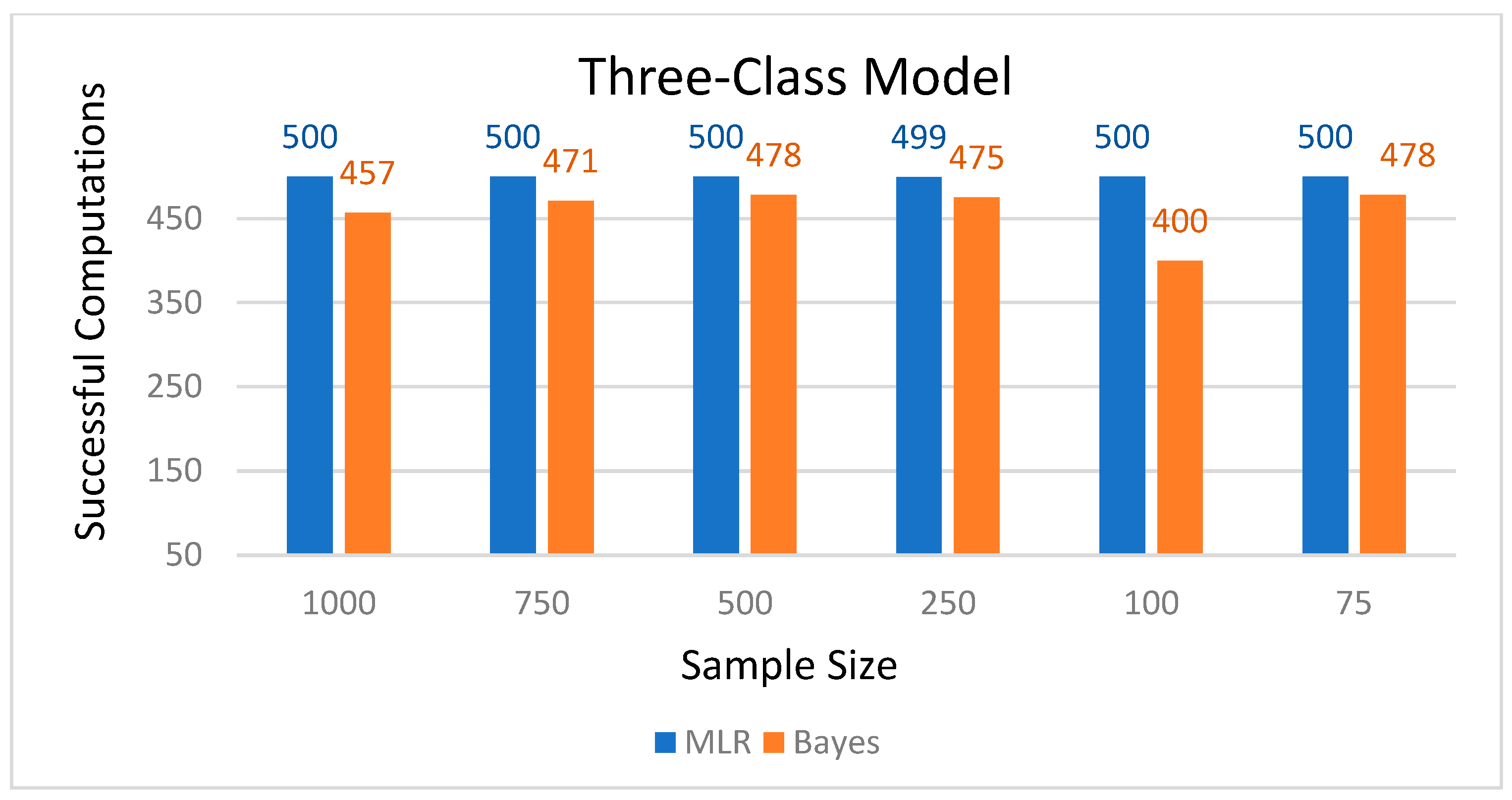
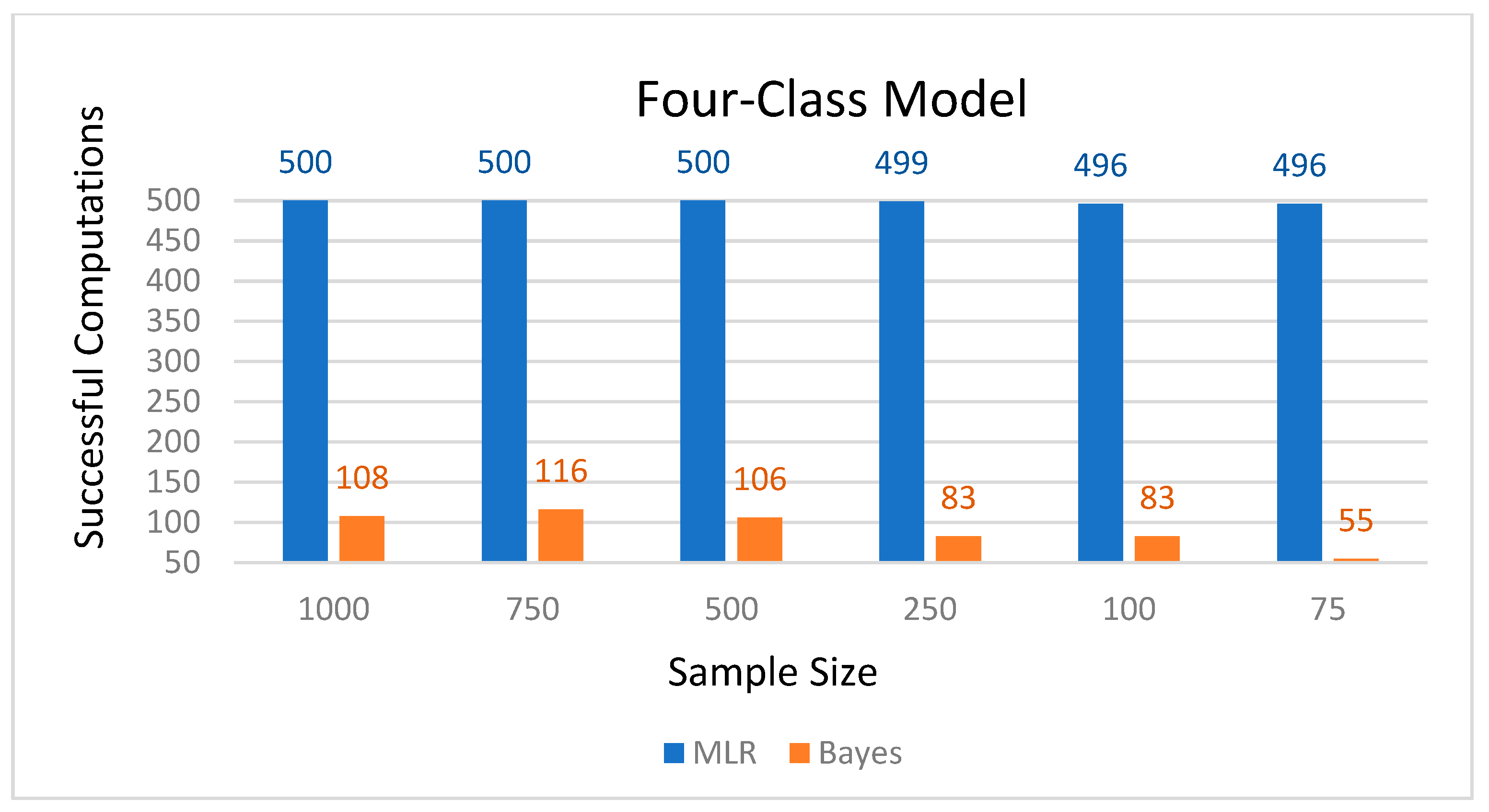
52]. The present study used MCMC simulations to compare Bayes and MLR classification precision under the same conditions. Specifically, the researcher compared three LCA models (with 2, 3, and 4 latent classes) measured by four binary observed indicators. The three LCA models were estimated using the Bayes with non-informative priors and the MLR procedures using samples of 1000, 750, 500, 250, 100, and 75 observations (3 × 2 × 6) with 500 replications. Entropy and average latent class probabilities were recorded and compared for each condition. The researcher used the M
plus 8.0 statistical package to conduct all analyses. The code for Monte Carlo simulations followed example 7.3 from the M
plus User’s Guide [
37] for generating a categorical latent variable with binary indicators. The example was modified to vary the sample sizes, the estimation method, and the number of classes. A sample code for the two-class model with Bayes estimation and a sample of 500 observations is included below:
Title:
Example of LCA model with binary;
latent class indicators using automatic;
starting values with random starts;
Montecarlo:
NAMES = u1-u4;
generate = u1-u4(1);
categorical = u1-u4;
genclasses = c(2);
classes = c(2);
nobs = 500;
seed = 3454367;
nrep = 500;
save = resultsfile.dat;
Analysis:
type = mixture;
estimator bayes;
Model population:
%overall%
[c#1*1];
%c#1%
[u1$1*2 u2$1*2 u3$1*-2 u4$1*-2];
%c#2%
[u1$1*-2 u2$1*-2 u3$1*2 u4$1*2];
Model:
%overall%
[c#1*1];
%c#1%
[u1$1*2 u2$1*2 u3$1*-2 u4$1*-2];
%c#2%
[u1$1*-2 u2$1*-2 u3$1*2 u4$1*2];
Output:
tech8 tech9;
6. Discussion and Conclusions
There is a noticeable gap in the existing research literature when it comes to studying the classification precision of BLCA. Despite the growing popularity of Bayesian methods in various fields, such as psychology, sociology, and marketing, there has been relatively limited attention given to the evaluation and comparison of classification accuracy specifically within the context of BLCA.
While LCA itself has been extensively studied and applied, much of the existing research has focused on traditional frequentist estimation methods, such as maximum likelihood estimation. BLCA offers unique advantages, such as the ability to incorporate prior knowledge, handle missing data, and provide probabilistic inferences. However, there is a lack of comprehensive empirical studies that directly investigate the classification precision of BLCA and compare it to other estimation approaches.
The limited research in this area may be attributed to several factors. First, Bayesian methods, including B LCA, often require advanced statistical knowledge and specialized software, which may deter some researchers from exploring these techniques. Second, there may be a perception that the computational complexity and longer execution times associated with Bayesian estimation hinder the feasibility of large-scale studies. Additionally, the absence of standardized guidelines or benchmarks for assessing the classification precision of BLCA further contributes to the scarcity of research in this domain.
As a result, more empirical studies are needed to address this gap in the literature. Such studies could compare the classification accuracy of BLCA with other popular estimation methods, evaluate its performance across different sample sizes and data characteristics, and provide insights into the factors that may influence the precision of BLCA classifications. These investigations would not only enhance our understanding of the strengths and limitations of BLCA but also provide researchers and practitioners with valuable guidance for selecting appropriate estimation methods in latent class analysis.
The primary objective of this study was to address this gap in the literature by investigating and comparing the accuracy of classification between two existing estimation methods: MLR and Bayes. MLR is the default Mplus estimation procedure for categorical variables. Despite its assumed benefits, the Bayes option, which is also available, is less frequently used and needs to be specified in the Mplus code. The current study aimed to determine whether using the default estimation settings, as most users do, may impact LCA classification precision.
Evaluating the classification precision of Bayes and MLR was based on the measurement of entropy and the average latent class probabilities for the most likely latent class membership. The study used binary observed indicators and included samples of different sizes and models with two–four latent classes.
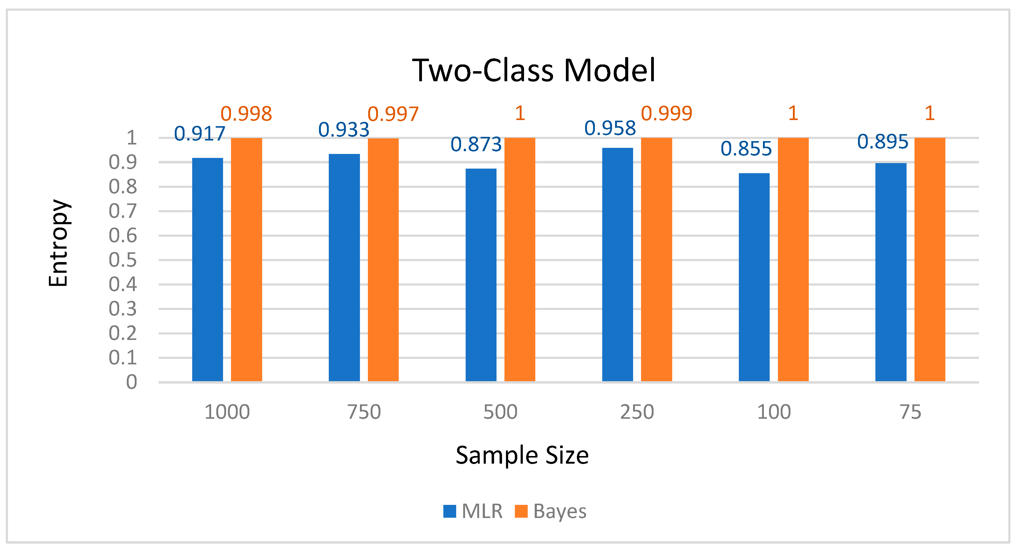
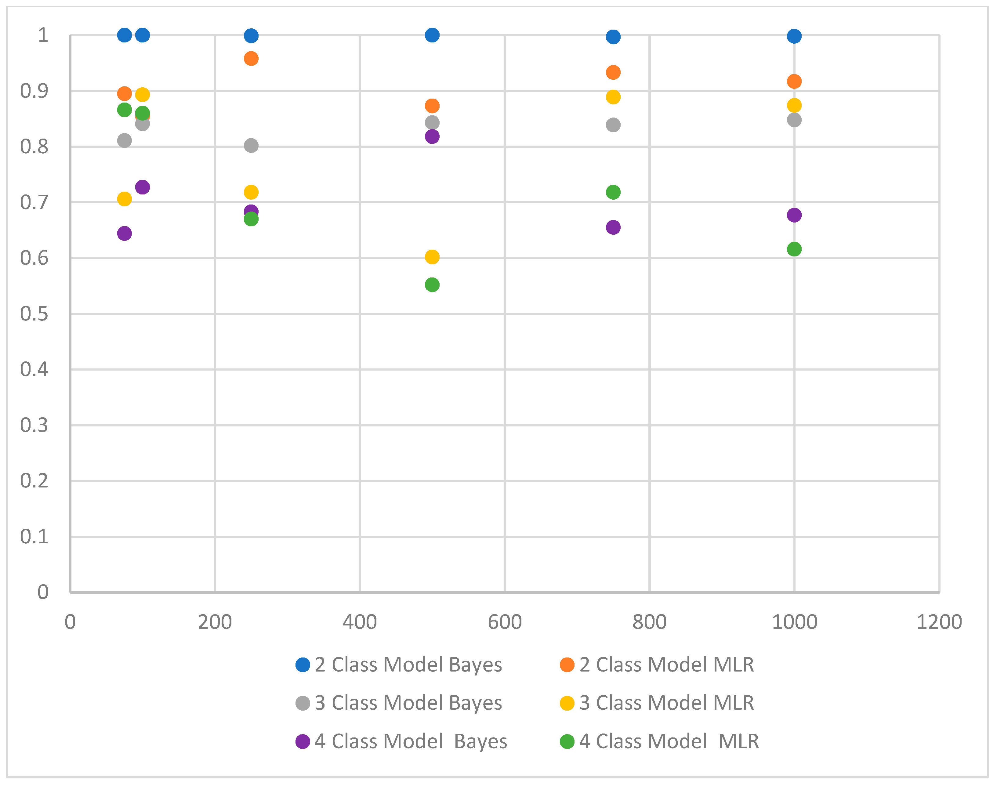
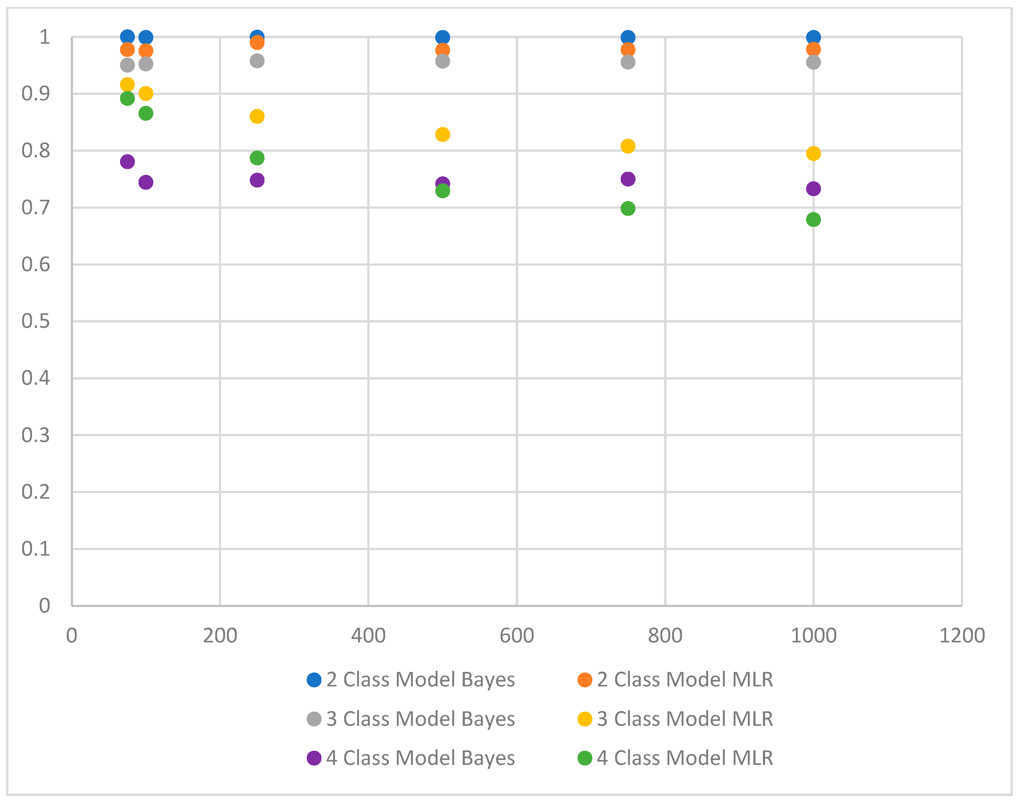
Results suggest that for models with two latent classes, regardless of sample size, the Bayes method consistently outperforms the MLR procedure. Specifically, Bayesian entropy values ranged between 0.997 and 1, whereas MLR entropy values ranged between 0.855 and 0.958. Similarly, Bayesian average latent class probabilities for latent class memberships ranged between 0.999 and 1, whereas and MLR average latent class probabilities ranged between 0.974 and 0.993.
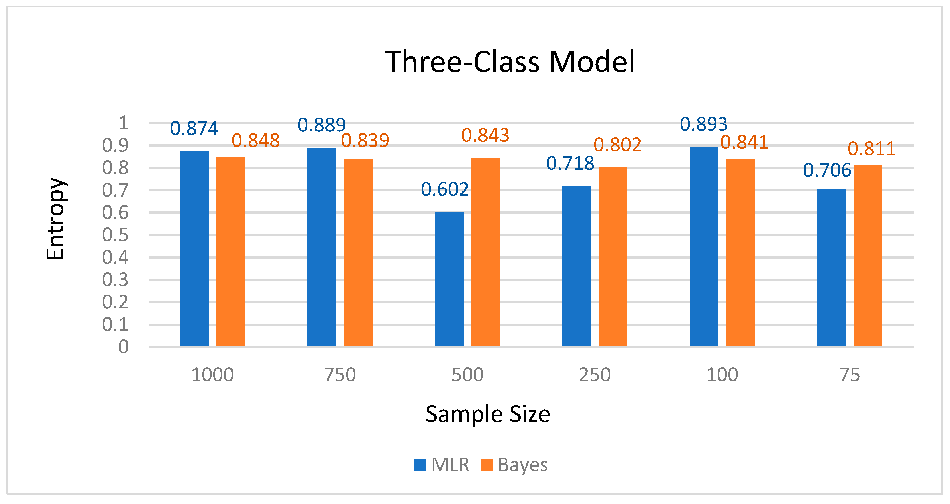
With three-class models, the Bayes method showed higher overall levels of classification precision with the sample of 75 (Bayesian entropy = 0.811, Bayes average latent class probabilities between 0.910 and 0.993; MLR entropy = 0.706, MLR average latent class probabilities between 0.905 and 0.922) and 500 samples (Bayesian entropy = 0.843, Bayesian average latent class probabilities between 0.940 and 0.993; MLR entropy = 0.602, MLR average latent class probabilities between 0.735 and 0.882). Nevertheless, the MLR procedure had slightly higher overall levels of classification precision with the larger samples (n = 750 and n = 1000). With the 750-sample size, the MLR entropy value was 0.889, whereas the Bayes entropy was 0.839; similarly, with the 1000-sample size, the MLR entropy was 0.874, whereas the Bayes entropy was 0.848.
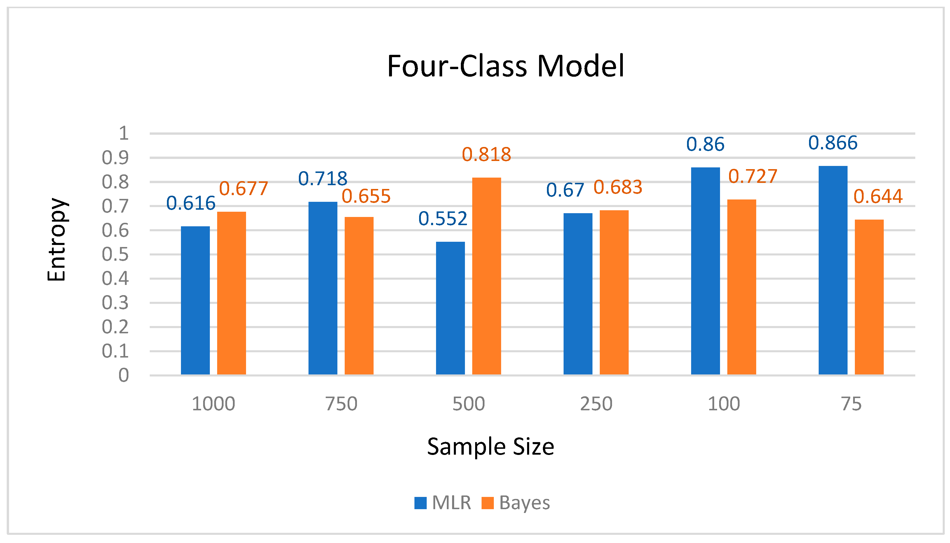
When the model included four classes, MLR outperformed Bayes estimation with smaller samples (n = 100 and n = 75). With the 75-sample size, MLR entropy was 0.866, and MLR average latent class probabilities ranged between 0.868 and 0.911, whereas the Bayes entropy was only 0.664 and Bayes average latent class probabilities ranged between 0.574 and 0.925. Similarly, with the 100-sample size, MLR entropy was 0.860, and average latent class probabilities ranged between 0.835 and 0.891, whereas Bayes entropy was 0.727, and average latent class probabilities ranged between 0.528 and 0.913.
Although some researchers suggest that the Bayes method may be more effective with smaller sample sizes [
43], results from the current study showed that this was only true for the smaller models, and classification precision varied mostly by model size than sample size. Overall, Bayes estimation provided more stable results, whereas MLR showed greater variations in average latent class probabilities for most likely latent class membership and entropy estimates. Nevertheless, the Bayes estimation had a much smaller number of successful computations than the four-class model. Furthermore, the Bayes estimation took extended time (days) with the four-class model. These computational difficulties may pose practical issues in using the Bayes procedure for applied research projects.
Based on these results, when working with binary observed indicators, researchers are advised to avoid deferring to the default Mplus settings and select an appropriate estimation procedure based on both sample size and model size. Specifically, with smaller models, users are advised to use the Bayes estimation, which seems to have greater classification precision even with very small samples. In contrast, as the number of classes specified in the LCA model increases, users can defer to MLR, particularly with smaller sample sizes. In these conditions, the Bayes method does not seem to yield the same level of classification precision as MLR and yields an increased number of unsuccessful computations.
In conclusion, the Bayesian procedure can benefit the classification precision of mixture models when models have fewer classes. Additionally, non-reliance on the assumption of independence may reduce estimation bias. Furthermore, the option to specify informative prior may increase estimation accuracy [
43]. Nevertheless, Bayesian estimation may encounter issues related to label switching [
4], lead to unsuccessful computations, and take extended time.
The essential contribution of this study is providing information on the classification precision LCA models with binary indicators using the Bayes and MLR estimation methods. Although some research in exploratory factor analysis indicates that this estimation method is effective with small sample sizes and ordinal data [
36], no research has assessed the precision of Bayes estimation for latent class models. Furthermore, the current study considered the complexity of the model by comparing models with different numbers of latent classes.
Although this information is helpful to applied researchers, this study is only a first step in comparing the effectiveness of the Bayes and MLR estimation procedures in latent class modeling. Additional simulation studies are needed to investigate the effectiveness of Bayes estimation compared to other estimators, such as maximum likelihood, and under other conditions, such as different types of observed indicators (ordered categorical, continuous, etc.), correctly specified versus miss-specified models, classes with varying prevalence, and with informative versus non-informative priors. Furthermore, we also encourage researchers to use BLCA with real data, particularly when estimating smaller LCA models.


