Statistical Inference of Burr–Hatke Exponential Distribution with Partially Accelerated Life Test under Progressively Type II Censoring

Abstract

In this paper, estimations of the parameter and acceleration factor of the Burr–Hatke exponential distribution in partially accelerated life tests under progressively type II censoring are investigated. By using typical maximum likelihood methods and the Bayesian method, point estimations of the distribution parameter and the acceleration factor are obtained. Based on the asymptotic normality and Delta method, approximate confidence intervals are established using the Fisher information matrix. The confidence intervals of the percentile bootstrap method are also evaluated. Comprehensive simulation tests are conducted to evaluate the estimations effects. A real dataset is studied by constructing a Burr–Hatke exponential model and analyzing the practicality and utility of parameter estimation.

1. Introduction

Life testing is an important approach to analyzing and evaluating the lifetime of a product which implicates the durability of the product. Life testing holds a significant position in reliability testing. The purpose of the life test can be generally categorized into three types:

(1) To find the life distribution of the product; (2) To obtain the statistical characteristics of the product’s life distribution; (3) To study the failure mechanism of the product.

The life test reveals the characteristics of the lifetime and failure mechanism of the product, which can be applied to make further reliability predictions and to improve the quality of the product. Therefore, life testing is crucial in modern industrial research.

According to the applied stress level, life tests can be classified into normal stress life tests and accelerated life stress tests. Normal stress life tests, namely, the traditional life test, collect data on the failure of the experimental object under normal conditions of use. For many reasons, such as the automation in the modern industry, the life span of products grows longer and it is hard to observe a sufficient number of product failures in a short period. Researchers accelerate the failure of the test object by changing the experimental conditions. Some common techniques include increasing the voltage and increasing the applied pressure.

The accelerated life stress test can be subdivided into a partially accelerated life test (PALT) and a fully accelerated life test (FALT). The difference between the two tests is whether all products are under increased stress. In a FALT, all products are under increased stress, which is also called the accelerated condition. During an accelerated life test, the experimenter would gather more failed units compared with the normal stress condition in a given amount of time. The researcher can extrapolate the lifetime characteristics of the product under normal stress from the lifetime and failure information of failed units under increased stress. To achieve this, it is necessary to find an index that reflects the magnitude of acceleration, called the acceleration factor, and then further build a physical model to describe the relationship between the acceleration factor and product life. Since the value of the acceleration factor is immeasurable and the life-stress model is not readily available in most cases, the partially accelerated life test (PALT) has a broader application than the fully accelerated life test (FALT). In PALT, experimental units were treated either under normal use stress conditions or accelerated stress conditions. Ref.  [1] divided the common life stress models into two categories: the step stress (SS) model and the constant stress (CS) model. In the CS life test, the units stay under a stabilized stress level, while in the SS life test, the pressure applied to the units increases step by step until the units break down.

The life test has two subcategories, one is called constant stress partial accelerated life test (CSPALT) and the other is called stepped stress partial accelerated life test (SSPALT). CSPALT and SSPALT are by far the most frequently used experimental methods in life testing. In CSPALT, units are always at normal use stress levels or fixed increased stress levels. This means that the stress level to which the sample is subjected does not change from the beginning of the test to the end of the test. Many studies on CSPALT have been conducted by scholars in recent years. Ref. [2] designed CSPALTs to estimate the parameters of the Burr XII distribution with multiple sets of type I and type II censored data. Ref. [3] assessed the superiority of estimates for CSPALTs using type I and type II censored data following Weibull distribution.

Censoring is a situation where an event occurs that is not observed or is not observable to the extent that the survival time cannot be accurately recorded. Censoring often needs to be factored into life tests. Right censoring usually occurs when a product survives longer than the observation time and is a frequent occurrence in lifespan tests. There are many different censoring schemes, and when the observation start time is the same, there are two types of censoring depending on the observation end time. For type I censoring, the observations of the remaining experimental subjects are uniformly cut off at a fixed time point, excluding the products that have failed. Type II censoring is that the observations are terminated when a predetermined amount of failure of the products is observed, and the percentage of censoring can be assumed to be predetermined. Due to the high reliability and long life of modern industrial products, a new censoring scheme, progressively type II censoring, is proposed. Consider a life test containing n units and a predetermined censoring ratio $S=\left(S_{j1},S_{j2},\dots ,S_{j{m}_j}\right)$. When the first product fails, $S_1$ units are randomly selected from the residual $n-1$ units and the observation on them is terminated; when the second product fails, $S_2$ units are randomly selected from the remaining $n-2-S_1$ units and the observation on them is terminated; and when the i product fails, $S_i$ units are randomly selected from the residual $n-i-S_1-S_2-\dots -S_{i-1}$ units and the observation on them is terminated. This censoring scheme can improve the efficiency of the experiment and reduce the cost, which can be seen in the case of [4,5].

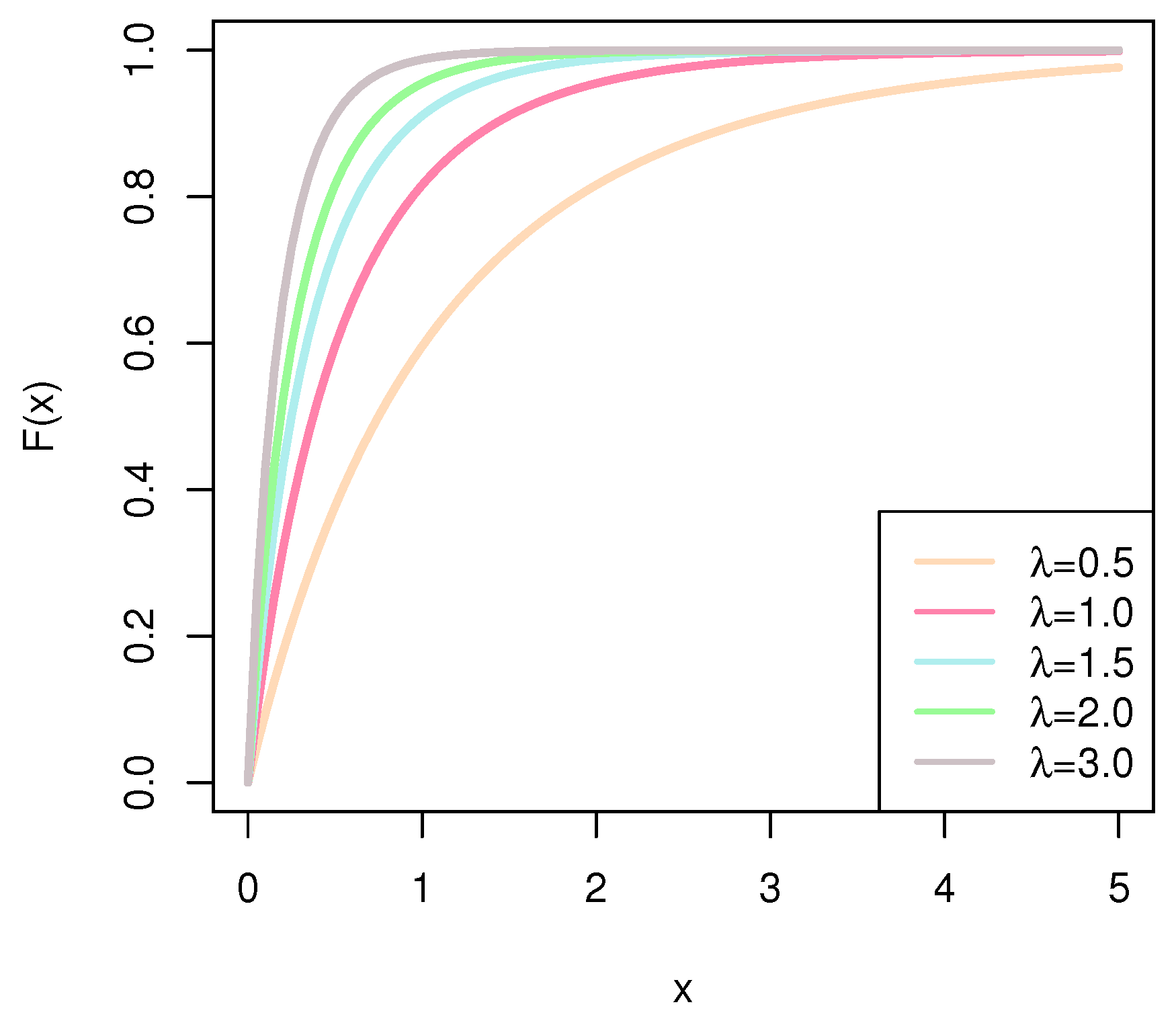
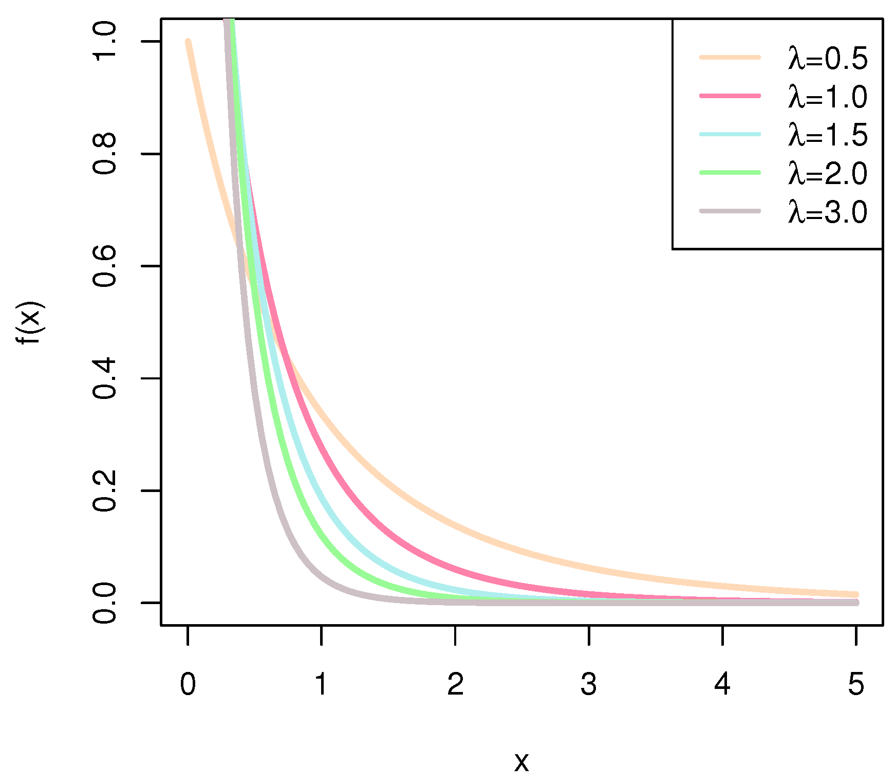
The exponential distribution is often used to establish models about life due to its memory-less property. Assume that X is an exponentially distributed random variable; then, the cumulative distribution function (CDF) and probability density function (PDF) are

$$\begin{array}{c}\hfill f\left(x\right)=\lambda e^{-\lambda x},\lambda >0,x>0\end{array}$$

(1)

$$\begin{array}{c}\hfill F\left(x\right)=1-e^{-\lambda x},\lambda >0,x>0\end{array}$$

(2)

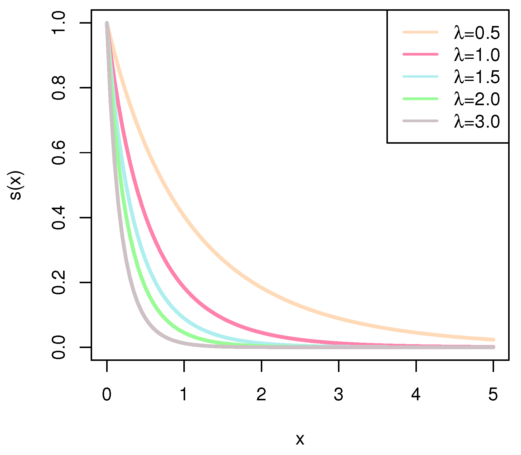
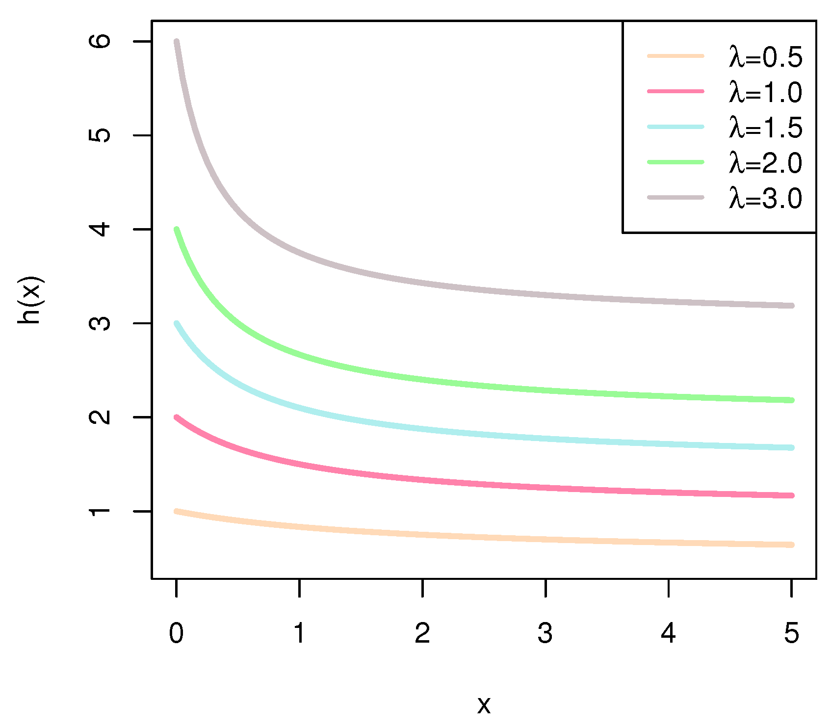
For the reliability analysis, the hazard rate function (HRF) describes the law of failure time and reflects the intensity of the probability of an individual’s instantaneous death at a point in time. The corresponding survival function (SF) represents the probability of an individual surviving. The HRF and SF are important tools for studying accelerated life tests and censored data. The expressions of the HRF and the SF of the exponential distribution are given by

$$\begin{array}{c}\hfill h\left(x\right)=\lambda ,\lambda >0,x>0\end{array}$$

(3)

$$\begin{array}{c}\hfill s\left(x\right)=e^{-\lambda x},\lambda >0,x>0.\end{array}$$

(4)

The HRF of the exponential distribution is a constant value function with the value $\lambda$.

Scholars have worked on mining other distributions as expanded extensions of the exponential distribution that can serve as models for simulating lifetimes. Ref. [6] generalized an exponentiated exponential distribution to develop a transmuted exponentiated exponential distribution. Ref. [7] introduced the Burr–Hatke–G family to simulate lifetimes.

The Burr–Hatke–G distribution family was constructed on the basis of the Burr–Hatke differential equation, which is given by

$$\begin{array}{c}\hfill \frac{dF}{dx}=g(x,F)F(1-F)\end{array}$$

(5)

$F\left(x\right)$ is a CDF of a continous random variable X, while $g\left(x,F\right)$ is any non-negative function. The Burr–Hatke–G family has attracted a lot of attention from scholars, such as [8,9]. Inspired by them, the authors of [10] proposed and analyzed a new lifetime distribution with one parameter, called the Burr–Hatke exponential (BHE) distribution, as an extension of the exponential distribution. Consider X as a random variable obeying Burr–Hatke exponential distribution. The cumulative distribution function, and probability density function, survival function, and hazard rate function of X can be formulated, respectively, as

$$\begin{array}{c}\hfill F_1\left(x\right)=1-\frac{e^{-\lambda x}}{1+\lambda x},\lambda >0,x>0\end{array}$$

(6)

$$\begin{array}{c}\hfill f_1\left(x\right)=\lambda e^{-\lambda x}\frac{2+\lambda x}{{(1+\lambda x)}^2},\lambda >0,x>0\end{array}$$

(7)

$$\begin{array}{c}\hfill S_1\left(x\right)=\frac{e^{-\lambda x}}{1+\lambda x},\lambda >0,x>0\end{array}$$

(8)

$$\begin{array}{c}\hfill H_1\left(x\right)=\lambda \frac{2+\lambda x}{1+\lambda x},\lambda >0,x>0\end{array}$$

(9)

The following Figure 1, Figure 2, Figure 3 and Figure 4 present the different images of CDF (6), PDF (7), SF (8), and HRF (9) when the parameter $\lambda$ takes different values.

The Burr–Hatke exponential distribution has good properties. Firstly, the moments of BHE are discussed. The first-order moment, mathematical expectation, and second-order moment are calculated as follows:

$$\begin{array}{c}\hfill E\left(X\right)=\mu =\frac{-\left(ϵe\right)}{\lambda }\end{array}$$

(10)

$$\begin{array}{c}\hfill E\left(X^2\right)=\frac{2\left(ϵe+1\right)}{{\lambda }^2}\end{array}$$

(11)

where

$$\begin{array}{c}\hfill ϵ={\int }_{-\infty }^{-1}{e}^t/tdt\end{array}$$

(12)

The variance (13) in BHE is easy to obtain.

$$\begin{array}{c}\hfill Var\left(X\right)=\frac{ϵe\left(2+ϵe\right)+2}{{\lambda }^2}\end{array}$$

(13)

Secondly, consider the asymptotics of BHE distribution. Let $a=inf\left\{x|F\left(x\right)>0\right\}$, when $x\to a$, the CDF, PDF, and HRF of BHE show the following convergence:

$$\begin{array}{c}\hfill F_{\lambda }\left(x\right)\sim 1-\left(-\lambda x\right)\end{array}$$

(14)

$$\begin{array}{c}\hfill f_{\lambda }\left(x\right)\sim \lambda e^{-\lambda x}\end{array}$$

(15)

$$\begin{array}{c}\hfill h_{\lambda }\left(x\right)\sim e^{-\lambda x}\end{array}$$

(16)

when $x\to \infty$, the asymptotics shows

$$\begin{array}{c}\hfill \left[1-F_{\lambda }\left(x\right)\right]\sim \frac{e^{-\lambda x}}{\lambda x}\end{array}$$

(17)

$$\begin{array}{c}\hfill f_{\lambda }\left(x\right)\sim \frac{\lambda \left(1-\lambda x\right)e^{-\lambda x}}{{\left(\lambda x\right)}^2}\end{array}$$

(18)

$$\begin{array}{c}\hfill h_{\lambda }\left(x\right)\sim \frac{\lambda \left(1-\lambda x\right)}{\lambda x}\end{array}$$

(19)

Notably, the HRF of BHE is a decreasing function, which can be seen in (9). The descending function describes the probability of breakdown reducing over time, which means improvement exists during the living time. Ref. [10] takes the opinion that it describes a situation where the probability of early death is high, and as time passes, the factors that could have caused the death initially reduce or disappear. In other words, there is some improvement in the sample that survives the initial period. Therefore, it may serve as a valuable model when analyzing data from reliability tests or medical fields that follow the decreasing pattern of HRF. Recently, much research on BHE has been conducted. Ref. [10] used the classical likelihood and Bayesian method to estimate a BHE model’s parameter, based on data under hybrid censoring, and confirmed that the BHE model fits both datasets well relative to other distributions. Ref. [11] estimated the BHE model parameter using the maximum likelihood method and considered BHE as an appropriate model for the right-skewed data. Ref. [12] considered a Burr–Hatke exponential distribution for a model of software development cost and analyzed the model by applying software failure time data. Ref. [9] using two real datasets illustrated that the BHE models fitted best compared with other models simulating lifetime empirically. Ref. [13] concluded that the BHE model is suitable in the field of software reliability analysis. Ref. [14] introduced the discrete BHE distribution and investigated its statistical properties insightfully.

In summary, this study of the Burr–Hatke exponential distribution has significant implications in practice. Studies of the Burr–Hatke exponential distribution on both accelerated life testing and under type II censoring are missing. The parameter of the BHE distribution under CSPALT with progressive type II censoring is estimated in this article. The maximum likelihood estimates (MLEs) and their approximate confidence intervals (ACIs) of the parameter and accelerated factor have been concluded. Interval estimates based on the Bootstrap method and point estimates calculated using the Bayesian method are also given.

The study in this paper fills the gap of BHE distribution in CSPALT, extends CSPALT to more applicable situations in life tests, and provides a new model for life test samples with reduced hazard rate functions.

This paper is organized as follows. In Section 2, the notation of the censored schemes and CSPALT is explained. In Section 3, the procedures to obtain maximum likelihood estimates and the Fisher information matrix are shown. The approximate confidence intervals using the delta method are built up. In Section 4, Boot-p confidence intervals based on Bootstrap methods are discussed. In Section 5, Bayesian point estimates are presented, using the Metropolis–Hasting algorithm for sampling. In Section 6, a Monte Carlo simulation study is performed to compare the implementation of the results of different estimates. In Section 7, a real dataset of oil breakdown times is analyzed to investigate the estimations of the parameters. In Section 8, the structure of the article is summarized and an outlook on the future work is provided.

2. Model Description

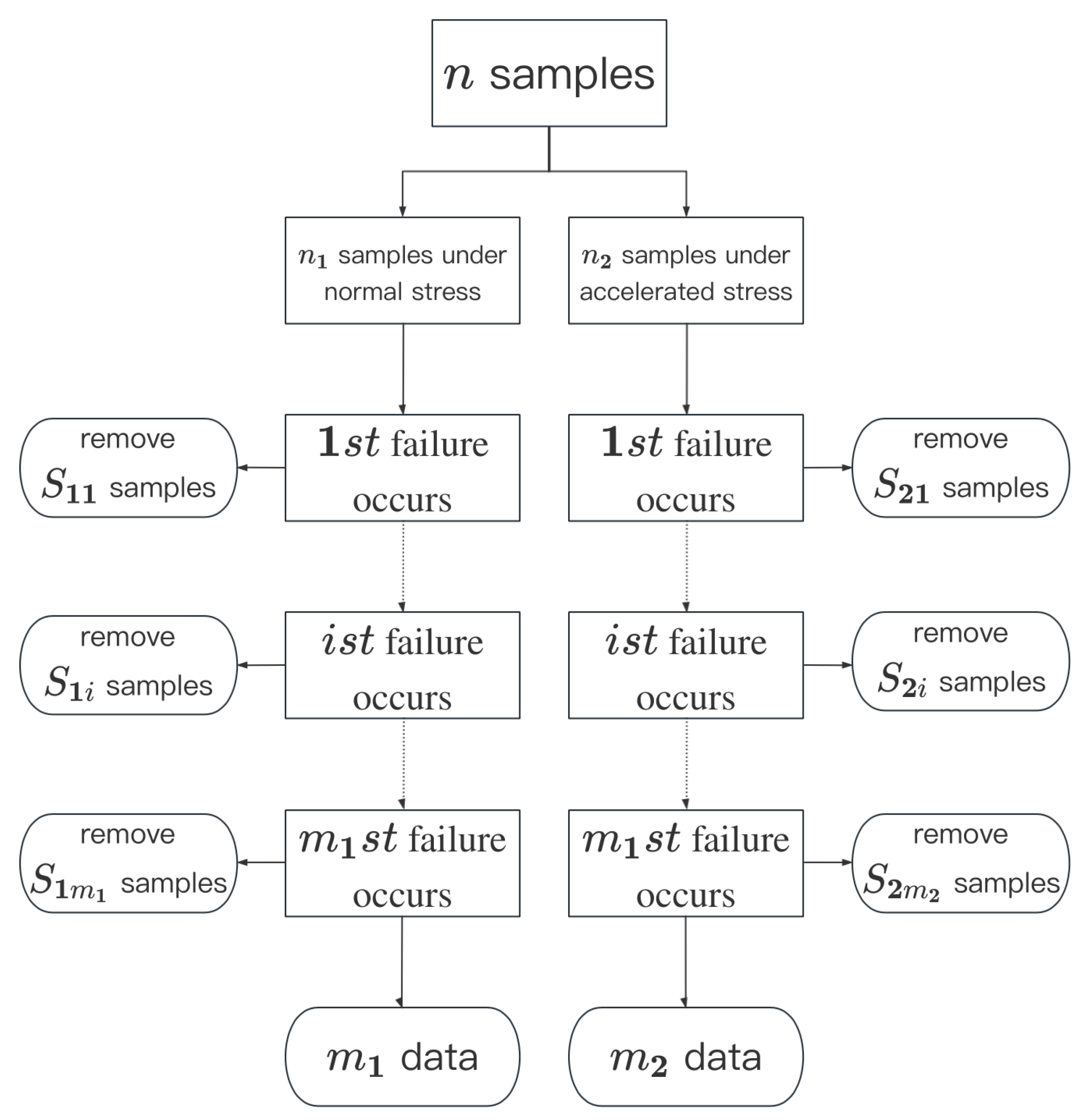
As a basis for subsequent estimation, the experimental approach to CSPALT under progressive type II censoring and the underlying assumptions about the model are as follows (Figure 5):

Assume that the total amount of samples is n. To build up a CSPALT test, randomly select an $n_1$ sample as test group 1, which is under normal stress, and the residual $n_2$, as group 2, is under the accelerated condition. Take progressively type II censoring into consideration, and set a sample size of $\left(n_j,m_j\right)$, where $j=1,2$ for each test group; then, $m_j$ is the observed number of failures for each test group. The prefixed censoring scheme is $(S_{j1},S_{j2},\dots ,S_{j{m}_j})$, which means that when the ith failure is observed, remove randomly selected $S_{ji}$ samples from the testing group.

Then, the observation is given by $\left(X_{j1},X_{j2},\dots ,X_{j{m}_j}\right),j=1,2$.

Several key assumptions are made as follows:

(1)

The lifetime of units in test group 1, under normal stress, follows a Burr–Hatke exponential distribution with CDF in (6), PDF in (7), SF in (8), and HRF in (9).

(2)

The HRF of units in test group 2, under the accelerated condition is given by $H_2\left(x\right)=\beta H_1\left(x\right)$, and $\beta$ is the acceleration factor that satisfies $\beta >1$.

Considering the above assumptions together, the HRF, SF, CDF, and PDF of the sample lifetime under accelerated stress conditions can be deduced with the following results.

$$\begin{array}{c}\hfill H_2\left(x\right)=\beta \lambda \frac{2+\lambda x}{1+\lambda x}\end{array}$$

(20)

$$\begin{array}{c}\hfill S_2\left(x\right)={\left(\frac{e^{-\lambda x}}{1+\lambda x}\right)}^{\beta }\end{array}$$

(21)

$$\begin{array}{c}\hfill F_2\left(x\right)=1-{\left(\frac{e^{-\lambda x}}{1+\lambda x}\right)}^{\beta }\end{array}$$

(22)

$$\begin{array}{c}\hfill f_2\left(x\right)=\beta \lambda e^{-\beta \lambda x}\frac{2+\lambda x}{{\left(1+\lambda x\right)}^{\beta +1}}\end{array}$$

(23)

The joint PDF of the observation $\left(X_{j1},X_{j2},\dots ,X_{j{m}_j}\right),j=1,2$ is the following.

$$\begin{array}{c}\hfill L\left(x\right)=\prod _{j=1}^2{A}_j\left\{\prod _{i=1}^{m_j}{f}_j\left(x_{ji}\right){\left[1-F_j\left(x_{ji}\right)\right]}^{S_{ji}}\right\}\end{array}$$

(24)

where

$$\begin{array}{c}\hfill A_j=n_j\left(n_j-1-S_{j1}\right)\left(n_j-2-S_{j1}-S_{j2}\right)\dots (n_j-m_j-\sum _{k=1}^{m_j-1}{S}_{jk}).\end{array}$$

(25)

3. Classical Inference

3.1. Maximum Likelihood Estimation

From the logarithm of the above joint density, neglecting the constant term and substituting the CDFs and PDFs, the log-likelihood function is defined to be

$$\begin{array}{ccc}\hfill l\left(\beta ,\lambda \right)& =& mlog\lambda +m_{2}log\beta -\sum _{i=1}^{m_1}\lambda \left(S_{1i}+1\right)x_{1i}+\sum _{i=1}^{m_1}\left[log\left(2+\lambda x_{1i}\right)-\left(S_{1i}+2\right)log\left(1+\lambda x_{1i}\right)\right]\hfill \\ & & -\sum _{i=1}^{m_2}\beta \lambda \left(S_{2i}+1\right)x_{2i}+\sum _{i=1}^{m_2}\left[log\left(2+\lambda x_{2i}\right)-\left(\beta S_{2i}+1+\beta \right)log\left(1+\lambda x_{2i}\right)\right]\hfill \end{array}$$

(26)

where $m=m_1+m_2$.

The MLEs of $\beta$ and $\lambda$ can be obtained by finding the partial derivatives of the log-likelihood function for $\beta$ and $\lambda$.

For a fixed $\lambda$, the MLE of $\beta$ is as follows:

$$\begin{array}{c}\hfill \widehat{\beta }\left(\lambda \right)=\frac{m_2}{{\sum }_{i=1}^{m_2}\lambda S_{2i}{x}_{2i}+{\sum }_{i=1}^{m_2}{S}_{2i}log\left(1+\lambda x_{2i}\right)}\end{array}$$

(27)

For a fixed $\beta$, the MLE of $\lambda$ can be derived from the following equation:

$$\begin{array}{ccc}\hfill \sum _{i=1}^{m_1}\left(S_{1i}+1\right)x_{1i}& +& \sum _{i=1}^{m_2}\left({\widehat{\beta }S}_{2i}+1\right)x_{2i}-\sum _{i=1}^{m_1}\left[\frac{x_{1i}}{2+\lambda x_{1i}}-\frac{\left(S_{1i}+2\right)x_{1i}}{1+\lambda x_{1i}}\right]\hfill \\ & & -\sum _{i=1}^{m_2}\left[\frac{x_{2i}}{2+\lambda x_{2i}}-\frac{\left({\widehat{\beta }S}_{2i}+2\right)x_{2i}}{1+\lambda x_{2i}}\right]=\frac{m}{\lambda }\hfill \end{array}$$

(28)

Proposition 1.

The solution of the equation about λ exists when and only when $m_1>0,m_2>0$.

To prove the existence of the solution of this equation, consider Function (29).

$$\begin{array}{ccc}\hfill G\left(\lambda \right)& =& \sum _{i=1}^{m_1}\left(S_{1i}+1\right)x_{1i}+\sum _{i=1}^{m_2}\left(\widehat{\beta }{S}_{2i}+1\right)x_{2i}-\sum _{i=1}^{m_1}\left[\frac{x_{1i}}{2+\lambda x_{1i}}-\frac{\left(S_{1i}+2\right)x_{1i}}{1+\lambda x_{1i}}\right]\hfill \\ & & -\sum _{i=1}^{m_2}\left[\frac{x_{2i}}{2+\lambda x_{2i}}-\frac{\left(\widehat{\beta }{S}_{2i}+2\right)x_{2i}}{1+\lambda x_{2i}}\right]-\frac{m}{\lambda }\hfill \end{array}$$

(29)

Consider first the continuity of $G\left(\lambda \right)$. Taking the derivative of $G\left(\lambda \right)$ with respect to $\lambda$, we have

$$\begin{array}{c}\hfill G\prime \left(\lambda \right)=\sum _{i=1}^{m_1}\left[\frac{{x_{1i}}^2}{{(2+\lambda x_{1i})}^2}-\frac{\left(S_{1i}+2\right){x_{1i}}^2}{{(1+\lambda x_{1i})}^2}\right]+\sum _{i=1}^{m_2}\left[\frac{{x_{2i}}^2}{{(2+\lambda x_{2i})}^2}-\frac{\left(\widehat{\beta }{S}_{2i}+2\right){x_{2i}}^2}{{(1+\lambda x_{2i})}^2}\right]+\frac{m}{{\lambda }^2}\end{array}$$

(30)

It can be concluded that $G\left(\lambda \right)$ is continuous when $\lambda >0$. Furthermore, observe the endpoint values of $G\left(\lambda \right)$.

As $\lambda \to 0$, we have

$$\begin{array}{ccc}\hfill G\left(\lambda \right)\to & & \sum _{i=1}^{m_1}\left(S_{1i}+1\right)x_{1i}+\sum _{i=1}^{m_2}\left(\widehat{\beta }{S}_{2i}+1\right)x_{2i}+\sum _{i=1}^{m_1}\left(\frac{3}{2}+S_{1i}\right)x_{1i}+\sum _{i=1}^{m_2}\left(\frac{3}{2}+\widehat{\beta }{S}_{2i}\right)x_{2i}-\frac{m}{\lambda }\hfill \\ & & =-\infty \hfill \end{array}$$

(31)

As $\lambda \to \infty$, we have

$$\begin{array}{c}\hfill G\left(\lambda \right)\to \sum _{i=1}^{m_1}\left(S_{1i}+1\right)x_{1i}+\sum _{i=1}^{m_2}\left(\widehat{\beta }{S}_{2i}+1\right)x_{2i}>0\end{array}$$

(32)

where $G\left(\lambda \right)$ is positive and negative at $\lambda \to 0$ and $\lambda \to \infty$, respectively. From the mid-value theorem, it can be seen that there exists $\lambda >0$ such that $G\left(\lambda \right)=0$ has a root. The existence of the estimate of $\lambda$ is proved.

3.2. Approximate Confidence Interval Estimation

Theorem 1.

Suppose that $x_1,\dots ,x_n$ are independent identically distributed samples from $f_{\theta }\left(x\right)$ and $\widehat{\theta }$ is the MLE of θ. Then,

$$\begin{array}{c}\hfill \widehat{\theta }\sim N(\theta ,\frac{I^{-1}\left(\theta \right)}{n})\end{array}$$

(33)

where $I\left(\theta \right)$ is the Fisher information matrix of θ.

Then, $\widehat{\lambda }$ and $\widehat{\beta }$ have the following asymptotic normal distribution.

$$\begin{array}{c}\hfill \widehat{\lambda }\sim N\left(\lambda ,var\left(\widehat{\lambda }\right)\right)\end{array}$$

(34)

$$\begin{array}{c}\hfill \widehat{\beta }\sim N\left(\beta ,var\left(\widehat{\beta }\right)\right)\end{array}$$

(35)

The approximate confidence intervals (ACIs) of the parameters can then be constructed, while a sufficiently large sample size is necessary.

The second-order partial derivatives of the maximum likelihood function are calculated and all partial second derivatives are obtained as follows.

$$\begin{array}{c}\hfill \frac{{\partial }^{2}l}{\partial {\beta }^2}=-\frac{m_2}{{\beta }^2}\end{array}$$

(36)

$$\begin{array}{c}\hfill \frac{{\partial }^{2}l}{\partial \beta \partial \lambda }=\frac{{\partial }^{2}l}{\partial \lambda \partial \beta }=-\sum _{i=1}^{m_2}(S_{2i}+1)x_{2i}\frac{2+\lambda x_{2i}}{1+\lambda x_{2i}}\end{array}$$

(37)

$$\begin{array}{c}\hfill \frac{{\partial }^{2}l}{\partial {\lambda }^2}=-\frac{m}{{\lambda }^2}+\sum _{i=1}^{m_1}\left[\frac{{-x_{1i}}^2}{{\left(2+\lambda x_{1i}\right)}^2}+\frac{\left(S_{1i}+2\right){x_{1i}}^2}{{(1+\lambda x_{1i})}^2}\right]+\sum _{i=1}^{m_2}\left[\frac{{-x_{2i}}^2}{{\left(2+\lambda x_{2i}\right)}^2}+\frac{\left(\beta S_{2i}+1+\beta \right){x_{2i}}^2}{{(1+\lambda x_{2i})}^2}\right]\end{array}$$

(38)

The variance–covariance matrix can be obtained from the Fisher information matrix, and their relationship equation is presented below.

$$\begin{array}{c}\hfill {I\left(\theta \right)}^{-1}=-{\left(\begin{array}{cc}\frac{{\partial }^{2}l}{\partial {\beta }^2}& \frac{{\partial }^{2}l}{\partial \beta \partial \lambda }\\ \frac{{\partial }^{2}l}{\partial \lambda \partial \beta }& \frac{{\partial }^{2}l}{\partial {\lambda }^2}\end{array}\right)}^{-1}=\left(\begin{array}{cc}var\left(\widehat{\beta }\right)& cov\left(\widehat{\beta },\widehat{\lambda }\right)\\ cov\left(\widehat{\lambda },\widehat{\beta }\right)& var\left(\widehat{\lambda }\right)\end{array}\right)\end{array}$$

(39)

Substituting the partial derivatives (36)–(38) into (39), the variances of $\widehat{\lambda }$ and $\widehat{\beta }$ are easily obtained.

Via the central limit theorem and the law of large numbers, the approximate 100$(1-\tau )\%$ confidence interval for parameter $\beta$, $\lambda$ is specified as

$$\begin{array}{c}\hfill \widehat{\beta }\pm Z_{\frac{\tau }{2}}\sqrt{var\left(\widehat{\beta }\right)}\end{array}$$

(40)

$$\begin{array}{c}\hfill \widehat{\lambda }\pm Z_{\frac{\tau }{2}}\sqrt{var\left(\widehat{\lambda }\right)}\end{array}$$

(41)

$Z_{\frac{\tau }{2}}$ is the $\frac{\tau }{2}$ quantile of the standard normal distribution.

Noting that the lower bound of the interval may be less than 0, the delta method proposed by [15] is adopted to construct more objective ACIs.

Proposition 2.

When a variable $\widehat{\beta }$ obeys the normal distribution, its function $g\left(\widehat{\beta }\right)$ obtained after the derivative transformation still obeys the normal distribution.

To ensure the non-negativity of the lower bound of ACI, let

$$\begin{array}{c}\hfill g\left(\beta \right)=log\left(\beta \right)\end{array}$$

(42)

It can be assumed that $g\left(\widehat{\beta }\right)$ obeys normal distribution according to the proposition (2). The expectation and variance in the new normal distribution can be derived by subjecting g to a Taylor expansion (43) on $\widehat{\beta }$.

$$\begin{array}{c}\hfill g\left(\widehat{\beta }\right)\approx g\left(\beta \right)+g\prime \left(\beta \right)(\widehat{\beta }-\beta )\end{array}$$

(43)

Substituting the functional expression of g into (43), we have the following:

$$\begin{array}{c}\hfill log\widehat{\beta }\sim Z\left(\beta ,\frac{var\left(\widehat{\beta }\right)}{{\beta }^2}\right)\end{array}$$

(44)

The $100(1-\tau )\%$ ACI for function $g\left(\widehat{\beta }\right)$ is presented as

$$\begin{array}{c}\hfill log\widehat{\beta }\pm Z_{\frac{\tau }{2}}\sqrt{\frac{var\left(\widehat{\beta }\right)}{{\beta }^2}}\end{array}$$

(45)

The new $100(1-\tau )\%$ ACI for parameter $\beta$ is given by

$$\begin{array}{c}\hfill (\widehat{\beta }{e}^{-Z_{\frac{\tau }{2}}\sqrt{\frac{var\left(\widehat{\beta }\right)}{{\beta }^2}}},\widehat{\beta }{e}^{Z_{\frac{\tau }{2}}\sqrt{\frac{var\left(\widehat{\beta }\right)}{{\beta }^2}}})\end{array}$$

(46)

Similarly, a more precise $100(1-\tau )\%$ ACI for $\lambda$ can be calculated, with the expression following.

$$\begin{array}{c}\hfill (\widehat{\lambda }{e}^{-Z_{\frac{\tau }{2}}\sqrt{\frac{var\left(\widehat{\lambda }\right)}{{\lambda }^2}}},\widehat{\lambda }{e}^{Z_{\frac{\tau }{2}}\sqrt{\frac{var\left(\widehat{\lambda }\right)}{{\lambda }^2}}})\end{array}$$

(47)

4. Bootstrap Confidence Intervals

The ACI is accurate only if the number of samples is large enough. When the number of samples is comparatively small, the accuracy of ACI may be lower and the bootstrap confidence interval (BCI) may have better results. Ref. [16] proposed a percentile bootstrap confidence interval (PBCI). To achieve both methods under progressively type II censoring, a simulation algorithm is needed. Ref. [4] proposed a simulation algorithm for generating a progressively type II censored sample from any continuous distribution. According to the type II censored generation algorithm, the specific steps to acquire the PBCI of parameters are as follows (Algorithm 1).

Algorithm 1: Percentile bootstrap confidence interval

1. A set of sample data from the experiment is the original experimental data. The MLEs  $\widehat{\lambda }$, $\widehat{\beta }$ of $\lambda$, $\beta$ are obtained by building the maximum likelihood function from the original experimental data. 2. Generate the progressively type II censored sample based on the MLEs $\widehat{\lambda }$, $\widehat{\beta }$ obtained  in step (1). 3. Establish the likelihood function concerning the progressively type II censored sample generated in step (2), calculate the MLEs ${\widehat{\lambda }}_1$, ${\widehat{\beta }}_1$ of $\lambda$, $\beta$. 4. Duplicate step (2) and step (3) up to B times to get $\left({\widehat{\lambda }}_1,{\widehat{\lambda }}_2,\dots ,{\widehat{\lambda }}_B\right)$, $\left({\widehat{\beta }}_1,{\widehat{\beta }}_2,\dots ,{\widehat{\beta }}_B\right)$. 5. Arrange the estimates of the parameters in step (4) in ascending order, we have $\left({\widehat{\lambda }}_{\left(1\right)},{\widehat{\lambda }}_{\left(2\right)},\dots ,{\widehat{\lambda }}_{\left(B\right)}\right)$, $\left({\widehat{\beta }}_{\left(1\right)},{\widehat{\beta }}_{\left(2\right)},\dots ,{\widehat{\beta }}_{\left(B\right)}\right)$.

    For arbitrary $0<\tau <1$, bilateral $100(1-\tau )\%$ percentile bootstrap confidence intervals for parameter $\lambda$ and $\beta$ can be composed in the following form.

$$\begin{array}{c}\hfill \left({\widehat{\lambda }}_{\left[\frac{B\tau }{2}\right]},{\widehat{\lambda }}_{\left[B\left(1-\frac{\tau }{2}\right)\right]}\right)\end{array}$$

(48)

and

$$\begin{array}{c}\hfill \left({\widehat{\beta }}_{\left[\frac{B\tau }{2}\right]},{\widehat{\beta }}_{\left[B\left(1-\frac{\tau }{2}\right)\right]}\right)\end{array}$$

(49)

where $\left[\frac{B\tau }{2}\right]$ represents the maximum integer less than $\frac{B\tau }{2}$; similarly, $\left[B\left(1-\frac{\tau }{2}\right)\right]$ represents the maximum integer less than $B\left(1-\frac{\tau }{2}\right)$.

5. Bayesian Estimation

Bayesian estimation is another important parameter estimation method. Unlike classical estimation, Bayesian estimation takes into account the randomness of the parameters, treating them as random variables rather than constants. The distribution of the parameters is used as prior information to make further statistical inferences more precise. In this section, point estimates based on the Bayesian theory and the highest posterior density credible intervals are obtained.

5.1. Bayesian Point Estimation

Firstly, consider the prior distribution of $\lambda$ and $\beta$. Due to the flexibility of the gamma distribution, we consider the gamma distribution as the prior distribution of the parameter $lambda$, i.e., $\lambda \sim Gamma\left(a_1,b_1\right)$. The hyperparameters $a_1,b_1$ are known positive constants. Considering the intuitiveness and accuracy of Bayesian estimation, we assume that lambda and beta are independent random variables, each following a distribution possessing the following density function:

$$\begin{array}{c}\hfill g\left(\lambda \right)={\lambda }^{a_1-1}{e}^{-b_1\lambda },\lambda >0\end{array}$$

(50)

$$\begin{array}{c}\hfill g\left(\beta \right)={\beta }^{-1},\beta >1\end{array}$$

(51)

The joint density function of $\lambda$ and $\beta$ is as follows:

$$\begin{array}{c}\hfill g\left(\lambda ,\beta \right)=\frac{{\lambda }^{a_1-1}{e}^{-b_1\lambda }}{\beta }\end{array}$$

(52)

The joint prior density function is thus obtained:

$$\begin{array}{ccc}\hfill & & {\lambda }^{m+a_1-1}{\beta }^{m_2-1}{e}^{-b_1\lambda }\times e^{-\lambda {\sum }_{i=1}^{m_1}(S_{1i}+1)x_{1i}}\prod _{i=1}^{m_1}\frac{(2+\lambda x_{1i})}{{(1+\lambda x_{1i})}^{(S_{1i}+2)}}\hfill \\ & & \times e^{-\lambda \beta {\sum }_{i=1}^{m_2}(S_{2i}+1)x_{2i}}\prod _{i=1}^{m_2}\frac{(2+\lambda x_{2i})}{{(1+\lambda x_{2i})}^{(\beta S_{2i}+S_{2i}+1)}}\hfill \end{array}$$

(53)

Putting forward the term associated with $\lambda$, the conditional posterior distribution is obtained as follows:

$$\begin{array}{c}\hfill {\lambda }^{m+a_1-1}{e}^{-b_1\lambda }{e}^{-\lambda {\sum }_{i=1}^{m_1}(S_{1i}+1)x_{1i}}\prod _{i=1}^{m_1}\frac{(2+\lambda x_{1i})}{{(1+\lambda x_{1i})}^{(S_{1i}+2)}}{e}^{-\lambda \beta {\sum }_{i=1}^{m_2}(S_{2i}+1)x_{2i}}\prod _{i=1}^{m_2}\frac{(2+\lambda x_{2i})}{{(1+\lambda x_{2i})}^{(\beta S_{2i}+S_{2i}+1)}}\end{array}$$

(54)

The conditional posterior distribution is obtained by taking the term related to $\beta$, as follows:

$$\begin{array}{c}\hfill {\beta }^{m_2-1}{e}^{-\beta (\lambda {\sum }_{i=1}^{m_2}(S_{2i}+1)x_{2i}+{\sum }_{i=1}^{m_2}(S_{2i}+1)log(1+\lambda x_{2i}))}\end{array}$$

(55)

It can be found that the posterior distribution of $\beta$ is a gamma distribution with parameters $m_2$ and $\lambda {\sum }_{i=1}^{m_2}(S_{2i}+1)x_{2i}+(S_{2i}+1){\sum }_{i=1}^{m_2}log(1+\lambda x_{2i})$, so the samples of beta can be generated directly using the gamma distribution. The posterior distribution of $\lambda$ is not a common distribution, and after a quick visualization, the figure is found to be similar to that of the normal distribution, so the sample of lambda is generated using the Metropolis–Hastings (MH) algorithm. The samples of $\lambda$ and $\beta$ are generated using the following Algorithm 2.

Algorithm 2: Bayesian estimates of $\lambda$ and $\beta$

1. Set the starting value of the parameter ${\lambda }_0$. 2. Generate $\beta \sim Gamma\left(m_2,\left(\lambda {\sum }_{i=1}^{m_2}\left(S_{2i}+1\right)x_{2i}+\left(S_{2i}+1\right){\sum }_{i=1}^{m_2}log\left(2+\lambda x_{2i}\right)\right)\right)$,  as ${\beta }_1$. 3. Use $N({\lambda }_0,{\sigma }_1^2)$ as the trial cast density, where ${\sigma }_1^2=0.01$, to generate a random  candidate sample $\lambda$, substitute into the joint prior density, compute the proportion of the  function value of the candidate sample to the function value of ${\lambda }_0$ and denote as r, then  accept $\lambda$ as the new sample ${\lambda }_1$ with probabilityr. 4. Duplicate step (2) and step (3) up to M times to obtain ${\lambda }_1,{\lambda }_2,\dots ,{\lambda }_M$, ${\beta }_1,{\beta }_2,\dots ,{\beta }_M$.

    In the Bayesian parameter estimation, the squared error loss function is chosen as the loss function.

The Bayesian estimations of $\lambda$ and $\beta$ are obtained as follows:

$$\begin{array}{c}\hfill \widehat{\lambda }=\frac{{\sum }_{i=N}^M{\lambda }_i}{M-N}\end{array}$$

(56)

$$\begin{array}{c}\hfill \widehat{\beta }=\frac{{\sum }_{i=N}^M{\beta }_i}{M-N}\end{array}$$

(57)

while N is the annealing factor, aiming to eliminate the effect of inaccuracies at the beginning of the iteration.

5.2. Highest Posterior Density Credible Interval

In the previous section for Bayesian point estimation, $M-N$ samples of $\lambda$ and $\beta$ were generated separately through posterior distributions, and by sorting these samples in ascending order, we have $\left({\widehat{\lambda }}_{\left(1\right)},{\widehat{\lambda }}_{\left(2\right)},\dots ,{\widehat{\lambda }}_{\left(M-N\right)}\right)$, $\left({\widehat{\beta }}_{\left(1\right)},{\widehat{\beta }}_{\left(2\right)},\dots ,{\widehat{\beta }}_{\left(M-N\right)}\right)$. For arbitrary $0<\tau <1$, a bilateral $100(1-\tau )\%$ confidence interval for parameter $\lambda$, $\beta$ can be composed in the following form.

$$\begin{array}{c}\hfill \left({\widehat{\lambda }}_{\left[\left(M-N\right)\frac{\tau }{2}\right]},{\widehat{\lambda }}_{\left[\left(M-N\right)\left(1-\frac{\tau }{2}\right)\right]}\right)\end{array}$$

(58)

and

$$\begin{array}{c}\hfill \left({\widehat{\beta }}_{\left[\left(M-N\right)\frac{\tau }{2}\right]},{\widehat{\beta }}_{\left[\left(M-N\right)\left(1-\frac{\tau }{2}\right)\right]}\right)\end{array}$$

(59)

where $\left[\left(M-N\right)\frac{\tau }{2}\right]$ represents the maximum integer less than $\left(M-N\right)\frac{\tau }{2}$; similarly, $[\left(M-N\right)$

$\left(1-\frac{\tau }{2}\right)]$ represents the maximum integer less than $\left(M-N\right)\left(1-\frac{\tau }{2}\right)$.

Repeat the above steps $N^{*}$ times to obtain $N^{*}$ interval estimates with the form above, from which the interval with the smallest length is selected as the highest posterior density credible interval.

6. Simulation Study

In this section, Monte Carlo simulations were conducted to judge the performance of the several methods mentioned above on parameter estimation.

Two sets of parameters are evaluated, as follows:

(1)

$\left(\lambda =1,\beta =2\right)$ with corresponding hyperparameters $\left(a_1=0.5,b_1=0.5\right)$.

(2)

$\left(\lambda =2.5,\beta =3.4\right)$ with corresponding hyperparameters $\left(a_1=1,b_1=0.4\right)$.

The value of the hyperparameter has a negligible effect on the results when the number of tests is large enough, so the value that makes the mean of the prior distribution the same as the original mean is chosen. Based on the theory part of the equation, the two sets of parameters are estimated separately. For all the interval estimates, the significant level is set at $\tau =0.05$.

To ensure the reliability of the test, six distinct sets of censoring schemes and sample sizes are selected:

(1)

$n_j=15,m_j=10,S_{j1}=5,S_{j2}=\dots =S_{j5}=0$

(2)

$n_j=15,m_j=10,S_{j1}=\dots =S_{j4}=0,S_{j5}=5$

(3)

$n_j=30,m_j=20,S_{j1}=10,S_{j2}=\dots =S_{j10}=0$

(4)

$n_j=30,m_j=20,S_{j1}=\dots =S_{j9}=0,S_{j10}=10$

(5)

$n_j=60,m_j=40,S_{j1}=20,S_{j2}=\dots =S_{j40}=0$

(6)

$n_j=60,m_j=40,S_{j1}=\dots =S_{j39}=0,S_{j40}=20$

In the process of algorithm implementation, data following the BHE distribution under progressively type II censoring need to be generated as samples. Progressively type II censored data are generated via the following Algorithm 3 proposed by [4].

Algorithm 3: Progressively type II censored data

1. Generate m independent samples $U_1,U_2,\dots ,U_m$ from $Uniform\left(0,1\right)$. 2. Set $Y_i={U_i}^{1/\left(i+S_m+S_{m-1}+\dots +S_{m-i+1}\right)}$, where $i=1,2,\dots ,m$.  $S=(S_1,S_2,\dots ,S_m)$ is  the censored scheme. 3. Set $Z_i=1-Y_m{Y}_{m-1}\dots Y_{m-i+1}$, where $i=1,2,\dots ,m$. Then $Z_1,Z_2,\dots ,Z_m$ are the progressively type II censored samples from $Uniform\left(0,1\right)$. 4. Calculate $X_i=F^{-1}\left(Z_i\right)$, where $i=1,2,\dots ,m$.  $F^{-1}\left(•\right)$ is the inverse of the aimed distribution function. Then $X_1,X_2,\dots ,X_m$ are the progressively type II censored samples derived from the distribution with $F\left(•\right)$.

Applying the expressions for the CDF under normal stress (6) and under accelerated stress (22) to the above algorithm, progressively type II censored data under normal use stress and accelerated stress conditions are produced. The complete experimental data of the simulated CSPALT are available and used to compare the superiority and inferiority of the parameter estimation methods.

The performance of the proposed methods for estimates of the BHE distribution based on the CSPALT under progressively type II censoring is verified via Monte Carlo simulation using the R-package. In the framework of classical maximum likelihood, the maximum likelihood function is solved using the Newton–Raphson method, and the Hessian matrix is used to obtain the maximum likelihood estimates. In the optimization process, the beginning value of the parameters is a random selection. The matrix is inverted to obtain the variance in the estimates and to construct asymptotic interval estimates by combining asymptotic normality. The Bayesian estimators are obtained using the gamma prior of $\lambda$ and the non-informative prior of $\beta$. The MH algorithm and the Gibbs sampling are applied due to the posterior distribution being difficult to obtain.

Using maximum likelihood and the Bayesian method, estimates of $\lambda$ and $\beta$ are obtained in the form of point estimates. The interval estimates are calculated using the maximum likelihood method and the bootstrap method. For each method of estimation, 5000 simulations were executed.

The criteria for judging the estimation effectiveness are as follows. For point estimation, there are two evaluation criteria, as follows:

(1)

Mean square error (MSE), calculated as

$$\begin{array}{c}\hfill \frac{{\sum }_{i=1}^N{\left(\widehat{\lambda }-\lambda \right)}^2}{N}\end{array}$$

(60)

$$\begin{array}{c}\hfill \frac{{\sum }_{i=1}^N{\left(\widehat{\beta }-\beta \right)}^2}{N}\end{array}$$

(61)

(2)

Average bias (AB), which is calculated as

$$\begin{array}{c}\hfill \frac{{\sum }_{i=1}^N\left|\widehat{\lambda }-\lambda \right|}{N}\end{array}$$

(62)

$$\begin{array}{c}\hfill \frac{{\sum }_{i=1}^N\left|\widehat{\beta }-\beta \right|}{N}\end{array}$$

(63)

For interval estimation, the judgment criteria are as follows:

(1)

Coverage probability (CP), namely, the proportion of intervals containing the true values of parameters to all intervals;

(2)

Average length (AL), that is, the distance from the maximum value to the minimum value of the interval.

The results of point and interval estimation are reported in the following tables.

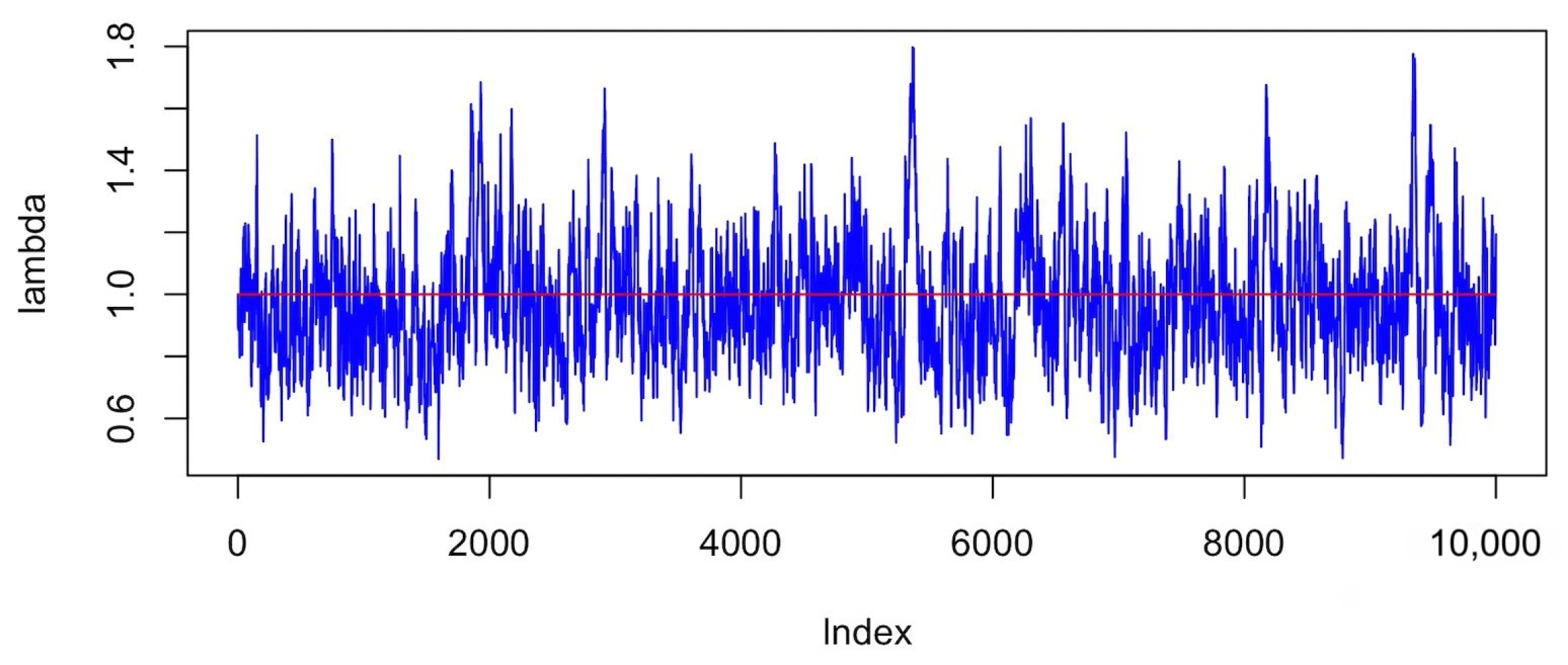
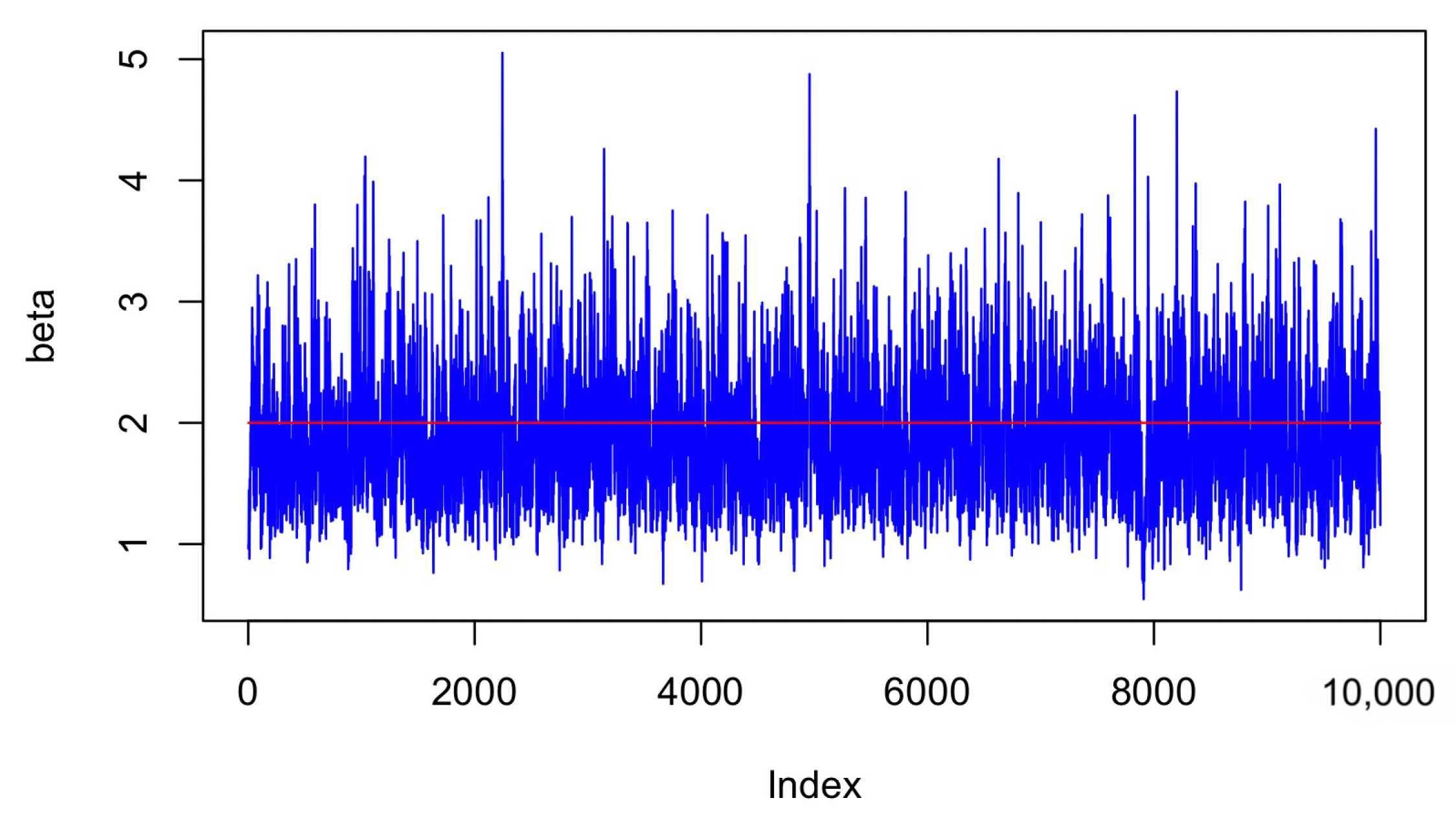
To represent the coverage of the intervals more intuitively, the BCI and PBCI are plotted separately as follows (Figure 6 and Figure 7), and it can be seen that both BCI and PBCL are good interval estimations.The red lines show the true values of the parameters.

From

Table 1. ABs and MSEs of unknown parameter and acceleration factor with ($\lambda$, $\beta$) = (1, 2).

	MLE		BE
CS	$\mathit{\lambda }$	$\mathit{\beta }$	$\mathit{\lambda }$	$\mathit{\beta }$
[1]	0.2683[0.1375]	0.7811[1.1713]	0.3725[0.2029]	0.8345[1.0440]
[2]	0.3155[0.1762]	0.8312[1.4896]	0.3498[0.1457]	1.2643[3.0430]
[3]	0.2117[0.0791]	0.5044[0.4055]	0.2525[0.0966]	0.5584[0.4499]
[4]	0.2043[0.0672]	0.5542[0.5871]	0.2259[0.0763]	0.6009[0.5706]
[5]	0.1473[0.0441]	0.4295[0.3270]	0.2242[0.0760]	0.4677[0.3278]
[6]	0.1662[0.0444]	0.4578[0.3512]	0.1814[0.0465]	0.4621[0.2914]

and

Table 2. ABs and MSEs of unknown parameter and acceleration factor with ($\lambda$, $\beta$) = (2.5, 3.4).

	MLE		BE
CS	$\mathit{\lambda }$	$\mathit{\beta }$	$\mathit{\lambda }$	$\mathit{\beta }$
[1]	0.7876[1.2247]	1.4158[4.2459]	1.8116[3.0753]	3.0276[8.3606]
[2]	0.7803[1.2886]	1.3835[3.8128]	1.7927[2.9894]	2.0089[7.3854]
[3]	0.5271[0.4971]	0.9560[1.6084]	1.7561[2.8364]	2.4469[5.5591]
[4]	0.5145[0.4817]	0.8967[1.4013]	1.9421[3.4317]	2.5794[6.1211]
[5]	0.4187[0.2997]	0.7512[0.9597]	1.8138[2.9991]	2.5852[6.1047]
[6]	0.3937[0.2780]	0.7817[1.0447]	1.5501[2.2273]	2.8741[3.7581]

, it can be seen that as the sample size $\left(n,m\right)$ increases, the values of MSEs and ABs, the statistics reflecting the centrality of MLEs and BEs, decrease, respectively. It can be assumed that the estimation has good consistency. The classical MLE estimation outperforms the Bayesian estimation when the censored scheme is fixed. For a fixed number of units $\left(n,m\right)$, the estimates of the censored scheme [1], [3], [5] are superior to the estimates of [2], [4], [6], namely, The censoring that happens following the initial observed failure provides more precise estimates compared with the others, which is consistent with the findings of [17].

From

Table 3. ALs and CPs of unknown parameter and acceleration factor with ($\lambda$, $\beta$) = (1, 2) with $\tau =0.05$.

	ACI		PBCI		HPD
CS	$\mathit{\lambda }$	$\mathit{\beta }$	$\mathit{\lambda }$	$\mathit{\beta }$	$\mathit{\lambda }$	$\mathit{\beta }$
[1]	1.5016[0.9510]	4.1679[0.9289]	1.5638[0.9424]	4.5314[0.9778]	[0.8190]	[0.9308]
[2]	1.5119[0.9540]	4.0603[0.9469]	1.5180[0.9424]	4.6190[0.9700]	[0.8712]	[0.9462]
[3]	1.0087[0.9560]	2.6996[0.9409]	1.0461[0.9388]	2.8309[0.9438]	[0.7658]	[0.9016]
[4]	1.0045[0.9540]	2.6503[0.9159]	1.0363[0.9360]	2.8157[0.9601]	[0.8710]	[0.9414]
[5]	0.8256[0.9479]	2.1376[0.9459]	0.8438[0.9470]	2.2186[0.9522]	[0.6284]	[0.8434]
[6]	0.7990[0.9459]	2.1728[0.9520]	0.8364[0.9480]	2.2241[0.9462]	[0.8368]	[0.9218]

For the HPD confidence intervals, we only present the coverage probability.

and

Table 4. ALs and CPs of unknown parameter and acceleration factor with ($\lambda$, $\beta$) = (2.5, 3.4) with $\tau =0.05$.

	ACI		PBCI
CS	$\mathit{\lambda }$	$\mathit{\beta }$	$\mathit{\lambda }$	$\mathit{\beta }$
[1]	1.5016[0.9510]	4.1679[0.9289]	4.0899[0.8560]	6.9612[0.8918]
[2]	1.5119[0.9540]	4.0603[0.9469]	3.9360[0.8588]	6.9319[0.8942]
[3]	1.0087[0.9560]	2.6996[0.9409]	2.7121[0.9272]	4.8121[0.9422]
[4]	1.0045[0.9540]	2.6503[0.9159]	2.6881[0.9220]	4.7897[0.9414]
[5]	0.8256[0.9479]	2.1376[0.9459]	2.1739[0.9418]	3.8547[0.9528]
[6]	0.7990[0.9459]	2.1728[0.9520]	2.1346[0.9528]	3.8671[0.9450]

, it can be seen that as the number of samples $\left(n,m\right)$ increases, the values of ALs of both ACIs and PBCIs decrease, respectively. The CPs of ACIs and PBCIs increase slightly, showing a tendency to converge to 95%, the values of the confidence interval.

In summary, both point estimates—the maximum likelihood estimate and the Bayesian estimate—show excellent performance, indicating the stability of both methods. The results of PBCI are poorer, and the estimation is also inefficient, requiring a long time to complete the iterations. The performance of ACI is much better than that of PBCI.

7. Real Data Analysis

In this section, real-time CSPALT life data are analyzed to further elaborate the estimation method described above. For additional clarification, we analyzed a real-time dataset of the oil breakdown time of insulating liquids. The life of many industrial components depends on the lifetime of electrical insulation. Accelerating conditions, such as turning up the voltage, can improve the efficiency of the life test. Ref. [1] studied accelerated tests based on this background, applying different magnitudes of voltage to different experimental groups for the tests. The data for the empirical analysis in this paper are derived from this study. Ref. [17], using this dataset and applying progressively type II censoring, compared the performance of several parameter estimations of Nadarajah–Haghighi distribution under CSPALT.

In the empirical analysis, the sample at 30 kV was used as data under the constant stress condition, and the sample at 32 kV was used as data under the accelerated stress condition. The data are presented as follows

Table 5. Real data set of oil breakdown times of insulating fluid under CSPALT recorded by [1].

Constant Stress Condition
194.902, 175.880, 144.120, 139.070, 47.300, 43.400, 22.660, 21.020, 20.460, 17.050, 7.740
Accelerated Stress Condition
215.10, 100.58, 89.29, 82.85, 53.24, 27.80, 15.93, 13.95, 9.88, 3.91, 2.75, 0.79, 0.69, 0.40 0.27

.

Before the estimation of parameters, the goodness-of-fit of the dataset to the BHE distribution was verified. Firstly, the Kolmogorov–Smirnov test (KS test) was used to measure the distance of the data from the distribution. 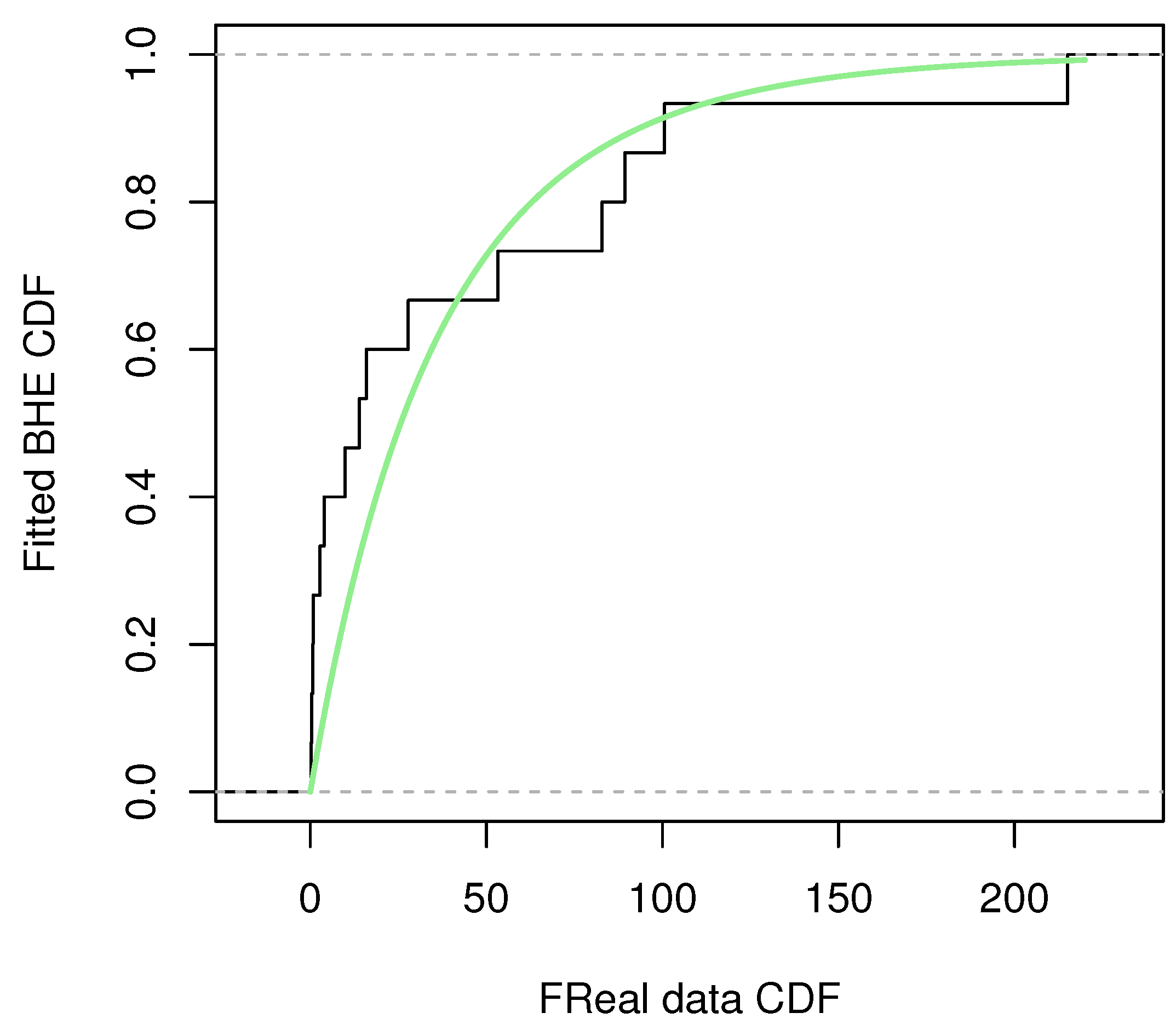The KS distance and p-value of data under the constant stress condition were calculated to be 0.2167 and 0.6062, respectively, and the KS distance and p-value of data under the accelerated stress condition were 0.2959 and 0.1167, respectively; at the significance level $\tau =0.05$, the dataset is considered suitable for fitting with the BHE distribution. 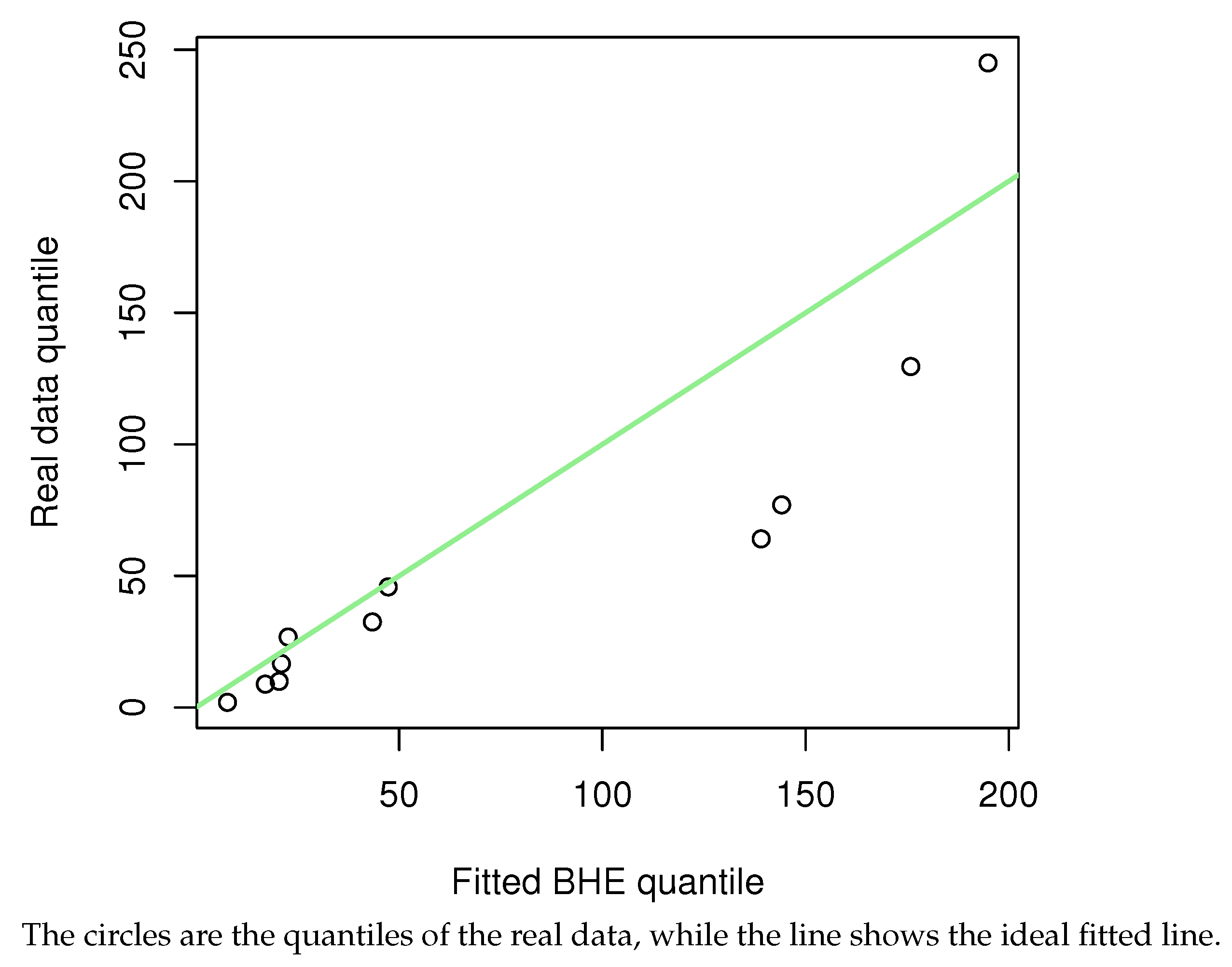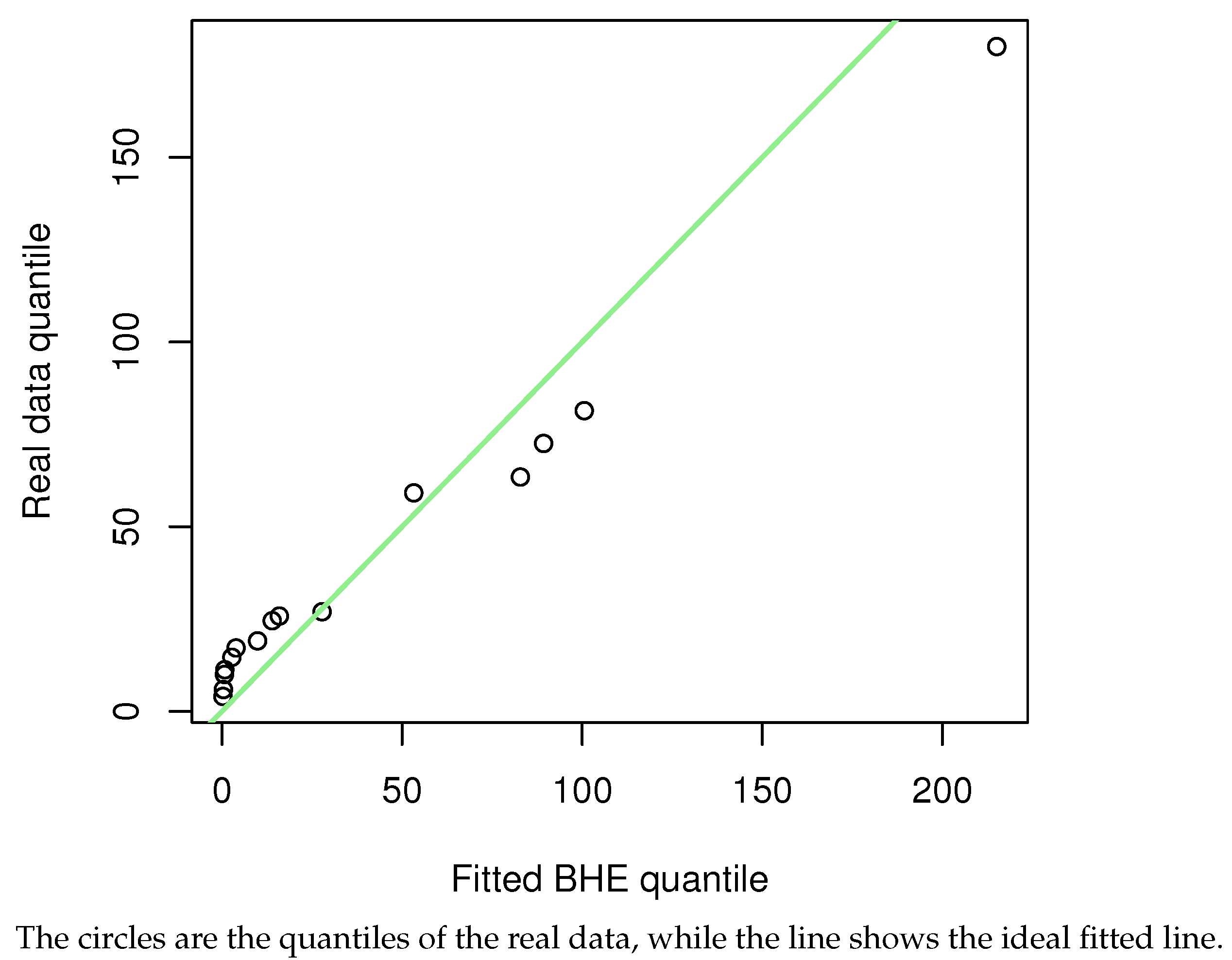To visualize how precisely this dataset fits the BHE distribution, a plot of the dataset‘s cumulative distribution with the CDF of BHE is shown in Figure 8 and Figure 9. The green line shows the CDF of BHE distribution. 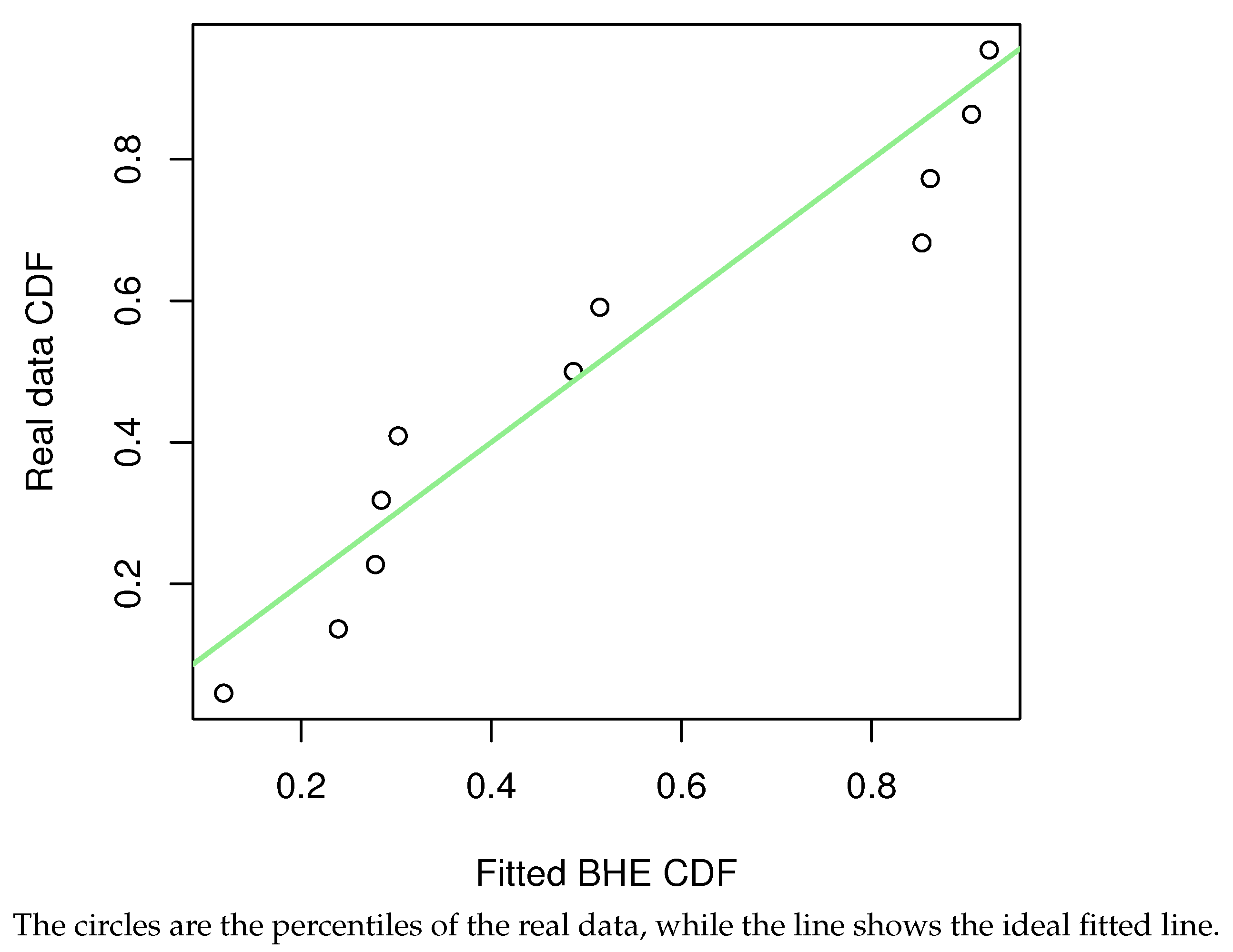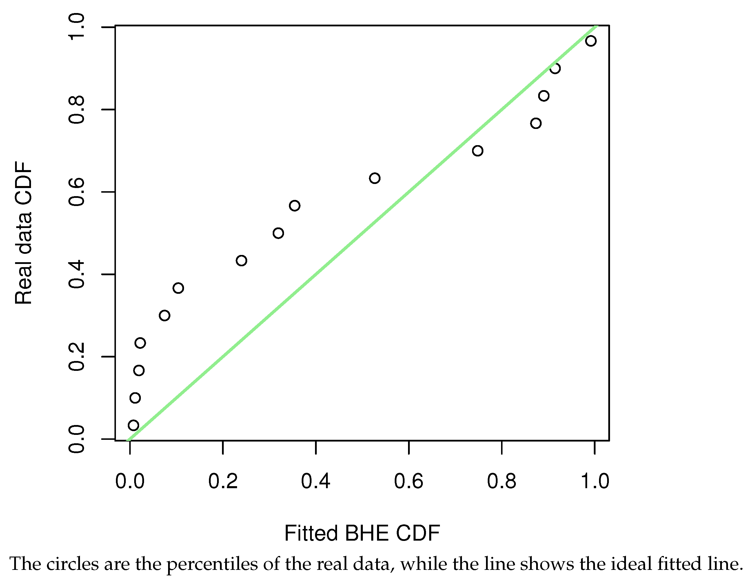Quantile–quantile plots (QQ plots) (Figure 10 and Figure 11) were further plotted, and the results were obtained as follows. The percentage–percentage plot (PP plot) (Figure 12 and Figure 13) are also presented. The conclusion is the same as the result of the KS test, that is, the model can be fitted using the BHE distribution for this dataset.

Considering the small sample size, a progressively type II censored scheme is selected with a small amount of censoring. The censored data are obtained as follows

Table 6. Censored data set of oil breakdown times of insulating fluid under CSPALT.

Constant Stress Condition $\left({\mathit{n}}_1,{\mathit{m}}_1\right)=\left(11,10\right){\mathit{S}}_1=\left(1,0,\mathit{\dots },0\right)$
7.74, 17.05, 20.46, 21.02, 43.40, 47.30, 139.07, 144.12, 175.88, 194.902
Accelerated Stress Condition $\left({\mathit{n}}_{\mathbf{2}},{\mathit{m}}_{\mathbf{2}}\right)=\left(\mathbf{15},\mathbf{14}\right){\mathit{S}}_{\mathbf{1}}=\left(\mathbf{1},\mathbf{0},\dots ,\mathbf{0}\right)$
0.27, 0.40, 0.69, 0.79, 2.75, 3.91, 9.88, 13.95, 15.93, 27.80, 53.24, 89.29, 100.58, 215.10

:

Under this assumption, point and interval estimates of the acceleration factor and the unknown parameter are obtained using the principles and algorithms in Section 3, Section 4 and Section 5. The results of parameter estimation are shown in the following

Table 7. Estimation of parameters of oil breakdown times of insulating fluid under CSPALT and progressively type II censoring.

	$\mathit{\lambda }$	$\mathit{\beta }$
MLE	0.0077	1.9802
BE	0.0076	1.9955
ACI	(0.0026,0.0127)[0.0101]	(0.4142,3.5462)[3.1320]
PBCI	(0.1980,3.3534)[3.1553]	(1.0000,3.4717)[2.4717]

.

In the Bayesian estimation, the parameter of the trial cast density normal distribution is chosen to be 0.001, and the hyperparameter of the gamma prior distribution is $\left(a_1,b_1\right)=\left(0.02,1\right)$, which matches the sample characteristics. The following conclusions can be obtained:

(1)

The results of MLE and BE are similar, indicating that the BHE model is consistent with the data.

(2)

The ACI of parameters $\lambda$ and $\beta$ contains the results of MLE and BE, and the length of the interval is small.

(3)

The results of PBCI with $\lambda$ illustrate the instability of PBCI, which is consistent with the conclusions in the Simulation Study section.

8. Conclusions

In the setting of Burr–Hatke exponential distribution, this paper investigates the process of parameter estimation for data from the partially accelerated life test (constant stress) after progressively type II censoring. The hazard function for the accelerated condition is derived from the fixed acceleration model, and the probability density function and cumulative distribution function are further derived. The joint density function of the data under constant stress condition and the data under accelerated stress condition are obtained, and the m likelihood estimates are obtained via the optimization theory. The approximate confidence intervals are constructed with the solution of the Fisher information matrix, while using percentiles in the bootstrap method, the bootstrap confidence intervals are obtained. The joint prior density was obtained by constructing the prior distribution of the parameters. The posterior distributions of the parameters were observed and the Bayesian point estimates were obtained using the Metropolis–Hastings algorithm. In the simulation test, constant stress partially conforming to the Burr–Hatke exponential distribution was generated from accelerated life test data and underwent progressively type-II censoring. The comparison shows that both maximum likelihood estimates and Bayesian estimates work well. It was also found that the approximate confidence interval outperformed the percentile bootstrap confidence intervals. Illustrative examples also confirm these conclusions. In future studies, more reasonable bootstrap confidence intervals will be explored. Interval estimation using the Bayesian method may show good results. It is also hoped that the parameter estimation can be extended to more distributions.

References

1. Nelson, W.B. Accelerated Testing: Statistical Models, Test Plans, and Data Analysis; John Wiley & Sons: Hoboken, NJ, USA, 2009. [Google Scholar]
2. Cheng, Y.F.; Wang, F.K. Estimating the Burr XII Parameters in Constant-Stress Partially Accelerated Life Tests under Multiple Censored Data. Commun. Stat.—Simul. Comput. 2012, 41, 1711–1727. [Google Scholar] [CrossRef]
3. Hassan, A.S.; Nassr, S.G.; Pramanik, S.; Maiti, S.S. Estimation in constant stress partially accelerated life tests for Weibull distribution based on censored competing risks data. Ann. Data Sci. 2020, 7, 45–62. [Google Scholar] [CrossRef]
4. Balakrishnan, N.; Sandhu, R.A. A Simple Simulational Algorithm for Generating Progressive Type-II Censored Samples. Am. Stat. 1995, 49, 229–230. [Google Scholar]
5. Balakrishnan, N.; Kannan, N.; Lin, C.T.; Wu, S.J.S. Inference for the extreme value distribution under progressive Type-II censoring. J. Stat. Comput. Simul. 2004, 74, 25–45. [Google Scholar] [CrossRef]
6. Merovci, F. Transmuted exponentiated exponential distribution. Math. Sci. Appl. Notes 2013, 1, 112–122. [Google Scholar]
7. Yousof, H.M.; Altun, E.; Ramires, T.G.; Alizadeh, M.; Rasekhi, M. A new family of distributions with properties, regression models and applications. J. Stat. Manag. Syst. 2018, 21, 163–188. [Google Scholar] [CrossRef]
8. Afify, A.; Aljohani, H.; Alghamdi, A.; Gemeay, A.; Sarg, A. A New Two-Parameter Burr-Hatke Distribution: Properties and Bayesian and Non-Bayesian Inference with Applications. J. Math. 2021, 2021, 1061083. [Google Scholar] [CrossRef]
9. El-Morshedy, M.; Aljohani, H.M.; Eliwa, M.S.; Nassar, M.; Shakhatreh, M.K.; Afify, A.Z. The Exponentiated Burr–Hatke Distribution and Its Discrete Version: Reliability Properties with CSALT Model, Inference and Applications. Mathematics 2021, 9, 2277. [Google Scholar] [CrossRef]
10. Yadav, A.S.; Altun, E.; Yousof, H.M. Burr–Hatke Exponential Distribution: A Decreasing Failure Rate Model, Statistical Inference and Applications. Ann. Data Sci. 2019, 8, 241–260. [Google Scholar] [CrossRef]
11. Abouelmagd, T. The logarithmic burr hatke exponential distribution for modeling reliability and medical data. Int. J. Stat. Probab. 2018, 7, 73–85. [Google Scholar] [CrossRef]
12. Kim, H.C. A Comparative Study on the Cost of Software Development Model Based on Burr–Hatke-Exponential Distribution. Int. J. Eng. Res. Technol. 2019, 12, 2036–2040. [Google Scholar]
13. Kyurkchiev, N. A Note on the Burr-Hatke-exponential Model. Some Applications. Compt. Rend. Acad. Bulg. Sci. 2021, 74, 488–495. [Google Scholar]
14. Pandey, A.; Singh, R.P.; Tyagi, A. An Inferential Study of Discrete Burr-Hatke Exponential Distribution under Complete and Censored Data. Reliab. Theory Appl. 2022, 17, 109–122. [Google Scholar] [CrossRef]
15. Cox, C. Encyclopedia of Environmetrics; John Wiley and Sons: Hoboken, NJ, USA, 2006. [Google Scholar]
16. Efron, B. The Jackknife, the Bootstrap and Other Resampling Plans; SIAM: Philadelphia, PA, USA, 1982. [Google Scholar]
17. Dey, S.; Wang, L.; Nassar, M. Inference on Nadarajah–Haghighi distribution with constant stress partially accelerated life tests under progressive type-II censoring. J. Appl. Stat. 2022, 49, 2891–2912. [Google Scholar] [CrossRef] [PubMed]
Figure 1. CDF of BHE.
Mathematics 11 02939 g001
Figure 2. PDF of BHE.
Mathematics 11 02939 g002
Figure 3. SF of BHE.
Mathematics 11 02939 g003
Figure 4. HRF of BHE.
Mathematics 11 02939 g004
Figure 5. CSPALT process.
Mathematics 11 02939 g005
Figure 6. Convergence of Bayesian estimation- λ .
Mathematics 11 02939 g006
Figure 7. Convergence of Bayesian estimation- β .
Mathematics 11 02939 g007
Figure 8. Constant stress condition.
Mathematics 11 02939 g008
Figure 9. Accelerated stress condition.
Mathematics 11 02939 g009
Figure 10. Constant stress condition.
Mathematics 11 02939 g010
Figure 11. Accelerated stress condition.
Mathematics 11 02939 g011
Figure 12. Constant stress condition.
Mathematics 11 02939 g012
Figure 13. Accelerated stress condition.
Mathematics 11 02939 g013