
An Ensemble Deep Learning Model for Provincial Load Forecasting Based on Reduced Dimensional Clustering and Decomposition Strategies

Abstract
:1. Introduction
2. Methodology
2.1. An Ensemble Forecasting Model Based on an Improved Load Clustering and Decomposition Strategy
2.2. Load Characteristic Dimensionality Reduction Based on Singular Value Decomposition (SVD)
2.3. K-Means Clustering Algorithm
- (1)
- Determine the number of clusters k according to the clustering validity index SSE.
- (2)
- Randomly select the initial k clustering centres u1, u2,……uk ∈ Rs. Calculate for each data sample the class lables it belongs to.
- (3)
- For each class j, recalculate the cluster centre of that class:where is the number of clustering centres recalculated for the t-th time for class i.
- (4)
- Update the class centre with the class mean.
- (5)
- Repeat (3) and (4) until the class centres are unchanged.
- (6)
- Output the clustering results.
2.4. Load Decomposition Based on VMD Algorithm
2.5. LSTM
2.6. CNN-GRU
2.6.1. CNN
2.6.2. GRU
2.7. Performance Evaluation
3. Case Analysis
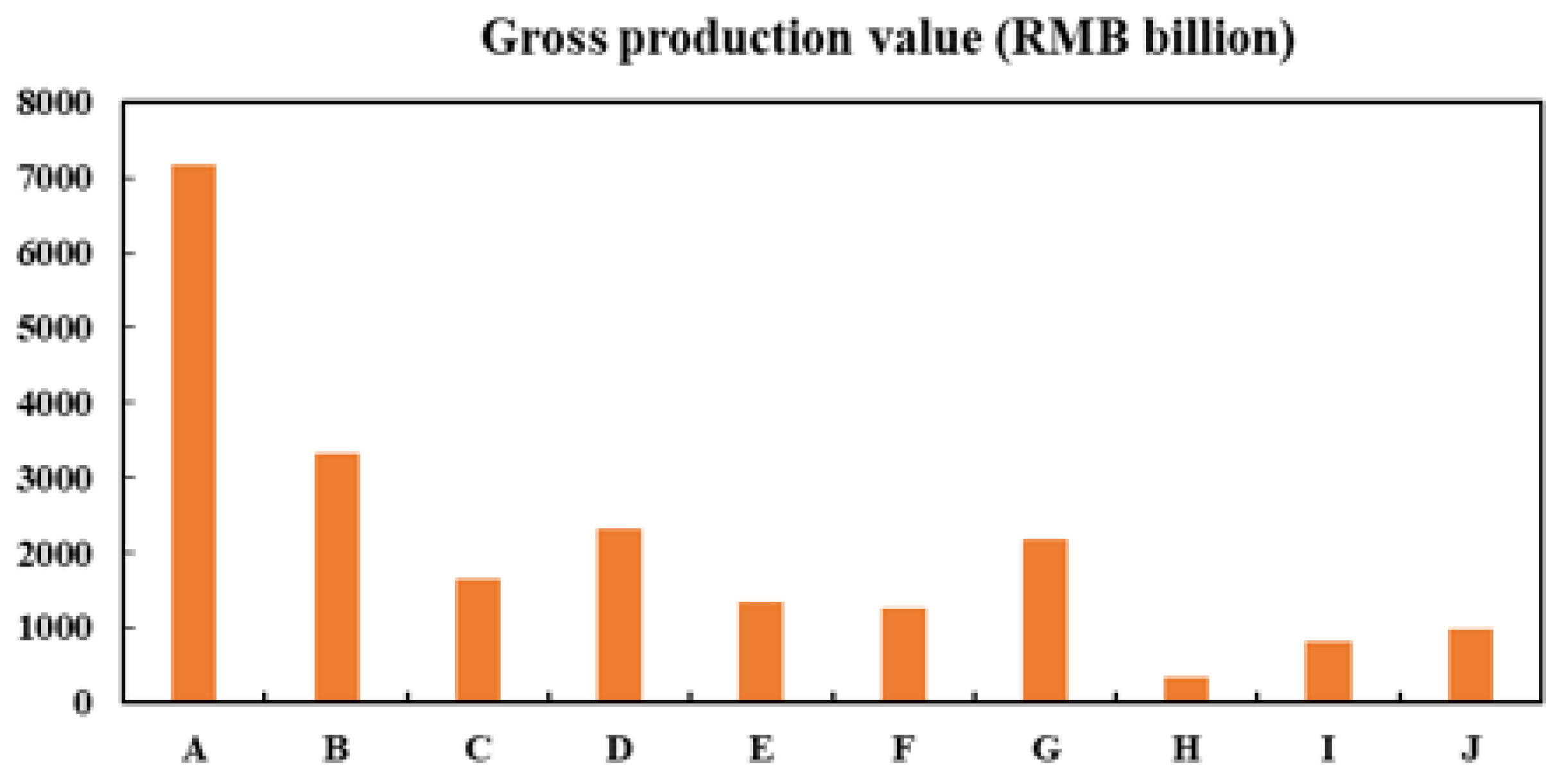
3.1. Load Characteristic Extraction
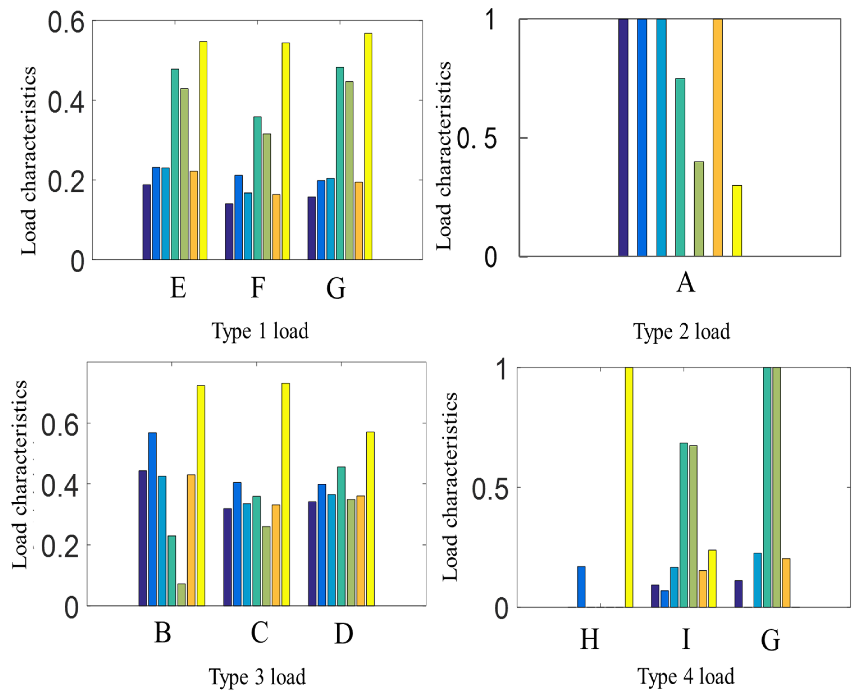
3.2. Analysis of Clustering Results for Ten City Loads
3.3. Analysis of the Results of the Frequency Domain Decomposition of the Load
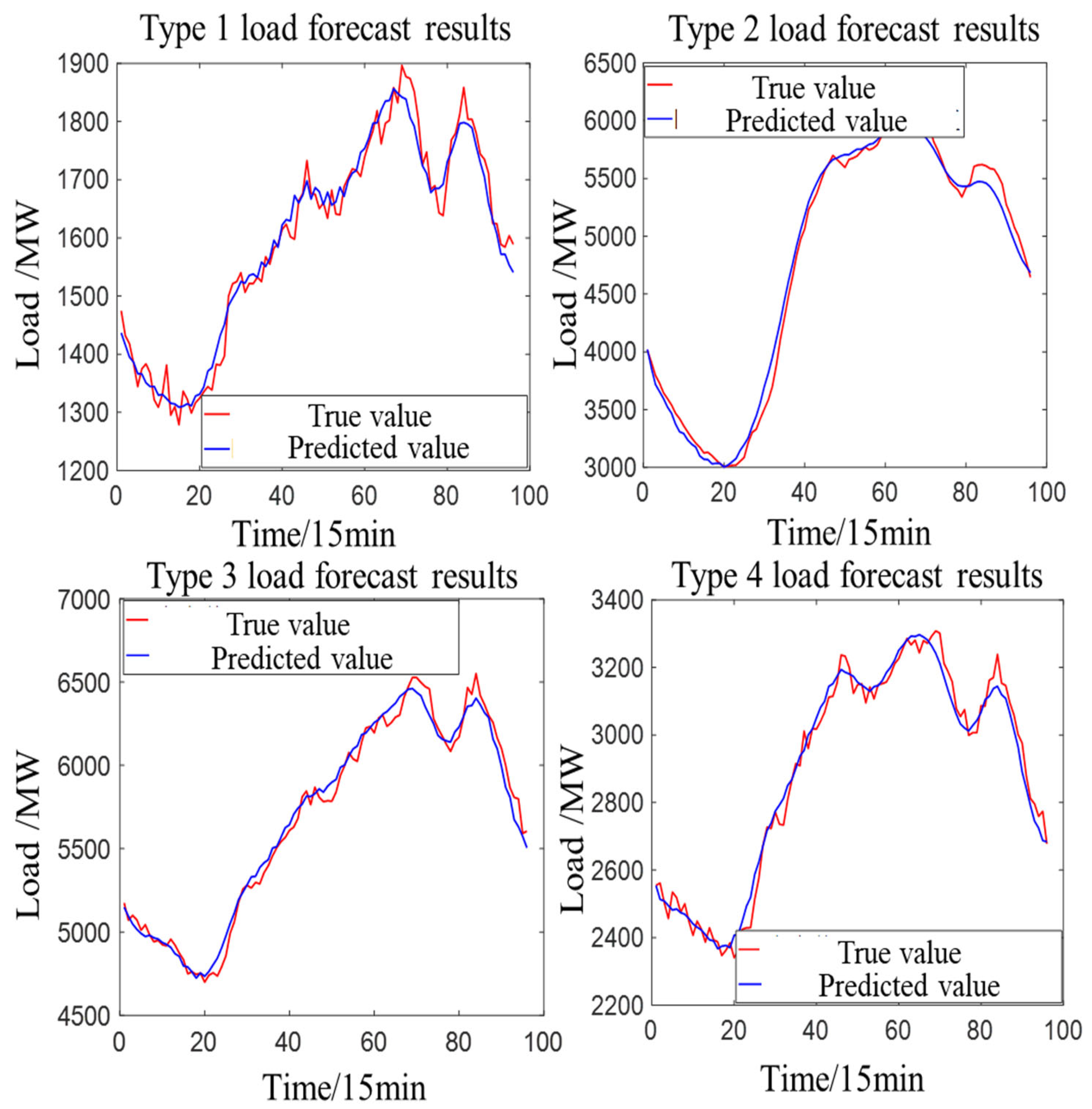
3.4. Analysis of Prediction Results Based on a Proposed Ensemble Model
3.5. Comparison of the Proposed Forecast and Baseline Schemes
3.5.1. Five Comparative Baseline Schemes
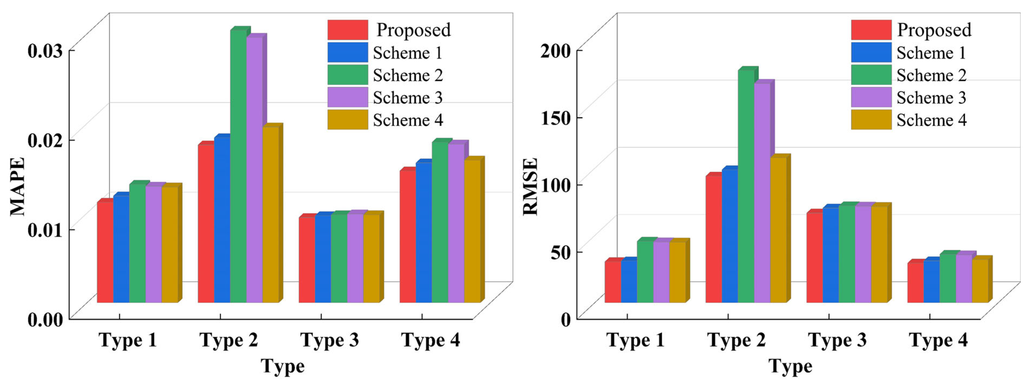
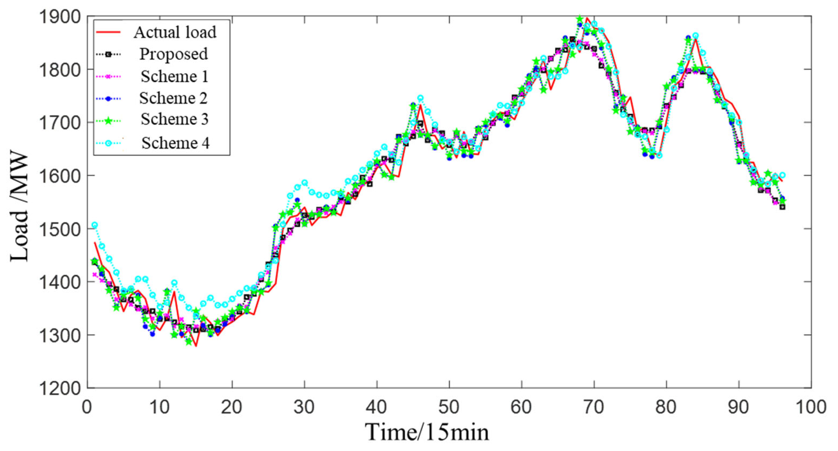
3.5.2. Comparison of Predictive Results for Various Types of Loads (Proposed Scheme and Schemes 1–4)
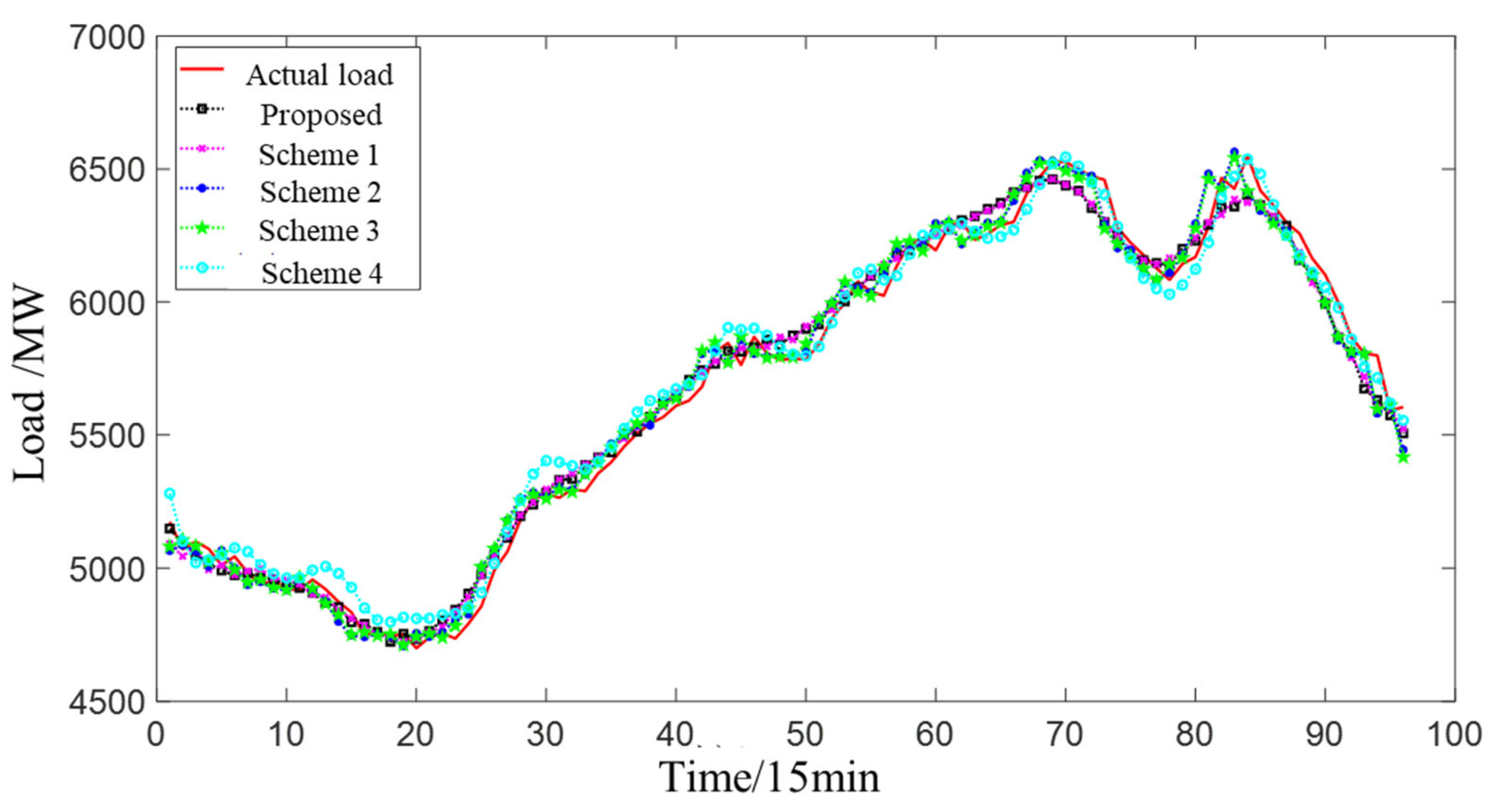
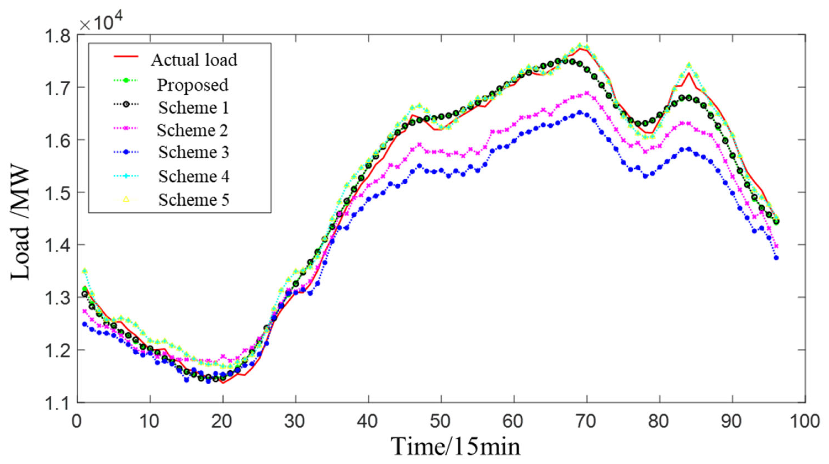
3.5.3. Comparison of the Predicted Results of the Total Provincial Load (Proposed Scheme and Schemes 1–5)
4. Conclusions
- (1)
- The proposed load clustering based on principal characteristic extraction improves the efficiency and quality of clustering. At the same time, the randomness of the load sequence for each class of users is reduced, as users with similar load characteristics are clustered into the same class. This reduces the complexity of load prediction and facilitates the improvement of prediction accuracy.
- (2)
- After VMD, the load sequence has a single frequency and is not prone to modal confusion. The VMD method can fully exploit the implicit features of the data and avoid the mutual interference between different local features. It lays the foundation for the accurate prediction of load sequences.
- (3)
- The proposed prediction model fully considers the fluctuation characteristics of high-frequency components and low-frequency components and fully utilizes the respective advantages of the LSTM and CNN-GRU models. At the same time, the total prediction error after the superposition of each class of load can offset the prediction error of each class to a certain extent, so that the prediction error after superposition can be further reduced. The results show that the proposed model can achieve better prediction results, and the proposed model can not only predict the change trend of electric load but also predict the local details. The forecast error (RMSE) of the proposed scheme is 0.23%, 63.49%, 75.84%, 1.59%, and 9.10% lower than that of the benchmark scheme.
- (4)
- The CNN-GRU component in the proposed model can better extract the local features of the high-frequency component, which ensures that the proposed model can track the load trend more accurately. Compared with the scheme that only uses LSTM to predict each frequency component, the proposed model increases the complexity of the model, but the prediction accuracy is improved.
Author Contributions
Funding
Data Availability Statement
Conflicts of Interest
References
- Wu, Z.; Mu, Y.; Deng, S.; Li, Y. Spatial–temporal short-term load forecasting framework via K-shape time series clustering method and graph convolutional networks. Energy Rep. 2022, 8, 8752–8766. [Google Scholar] [CrossRef]
- Yang, Y.; Zhou, H.; Wu, J.; Liu, C.-J.; Wang, Y.-G. A novel decompose-cluster-feedback algorithm for load forecasting with hierarchical structure. Int. J. Electr. Power Energy Syst. 2022, 142, 108249. [Google Scholar] [CrossRef]
- Yang, Y.; Wang, Z.; Gao, Y.; Wu, J.; Zhao, S.; Ding, Z. An effective dimensionality reduction approach for short-term load forecasting. Electr. Power Syst. Res. 2022, 210, 108150. [Google Scholar] [CrossRef]
- Haque, A.; Rahman, S. Short-term electrical load forecasting through heuristic configuration of regularized deep neural network. Appl. Soft Comput. 2022, 122, 108877. [Google Scholar] [CrossRef]
- Deng, X.; Ye, A.; Zhong, J.; Xu, D.; Yang, W.; Song, Z.; Zhang, Z.; Guo, J.; Wang, T.; Tian, Y.; et al. Bagging–XGBoost algorithm based extreme weather identification and short-term load forecasting model. Energy Rep. 2022, 8, 8661–8674. [Google Scholar] [CrossRef]
- Han, X.; Su, J.; Hong, Y.; Gong, P.; Zhu, D. Mid- to Long-Term Electric Load Forecasting Based on the EMD–Isomap–Adaboost Model. Sustainability 2022, 14, 7608. [Google Scholar] [CrossRef]
- Lee, G.-C. Regression-Based Methods for Daily Peak Load Forecasting in South Korea. Sustainability 2022, 14, 3984. [Google Scholar] [CrossRef]
- Zhao, X.; Shen, B.; Lin, L.; Liu, D.; Yan, M.; Li, G. Residential Electricity Load Forecasting Based on Fuzzy Cluster Analysis and LSSVM with Optimization by the Fireworks Algorithm. Sustainability 2022, 14, 1312. [Google Scholar] [CrossRef]
- Li, M.; Xie, X.; Zhang, D. Improved Deep Learning Model Based on Self-Paced Learning for Multiscale Short-Term Electricity Load Forecasting. Sustainability 2022, 14, 188. [Google Scholar] [CrossRef]
- Son, N. Comparison of the Deep Learning Performance for Short-Term Power Load Forecasting. Sustainability 2022, 13, 12493. [Google Scholar] [CrossRef]
- Aslam, S.; Ayub, N.; Farooq, U.; Alvi, M.J.; Albogamy, F.R.; Rukh, G.; Haider, S.I.; Azar, A.T.; Bukhsh, R. Towards Electric Price and Load Forecasting Using CNN-Based Ensembler in Smart Grid. Sustainability 2021, 13, 12653. [Google Scholar] [CrossRef]
- Wang, H.; Zhang, N.; Du, E.; Yan, J.; Han, S.; Liu, Y. A comprehensive review for wind, solar, and electrical load forecasting methods. Glob. Energy Interconnect. 2022, 5, 9–30. [Google Scholar] [CrossRef]
- Yang, D.; Guo, J.-E.; Li, Y.; Sun, S.; Wang, S. Short-term load forecasting with an improved dynamic decomposition-reconstruction-ensemble approach. Energy 2023, 263, 125609. [Google Scholar] [CrossRef]
- Geng, G.; He, Y.; Zhang, J.; Qin, T.; Yang, B. Short-Term Power Load Forecasting Based on PSO-Optimized VMD-TCN-Attention Mechanism. Energies 2023, 16, 4616. [Google Scholar] [CrossRef]
- Matrenin, P.; Safaraliev, M.; Dmitriev, S.; Kokin, S.; Ghulomzoda, A.; Mitrofanov, S. Medium-term load forecasting in isolated power systems based on ensemble machine learning models. Energy Rep. 2022, 8, 612–618. [Google Scholar] [CrossRef]
- Wang, S.; Wang, S.; Wang, D. Combined probability density model for medium term load forecasting based on quantile regression and kernel density estimation. Energy Procedia 2019, 158, 6446–6451. [Google Scholar] [CrossRef]
- Ahmad, T.; Zhang, H. Novel deep supervised ML models with feature selection approach for large-scale utilities and buildings short and medium-term load requirement forecasts. Energy 2020, 209, 118477. [Google Scholar] [CrossRef]
- Kalhori, M.R.N.; Emami, I.T.; Fallahi, F.; Tabarzadi, M. A data-driven knowledge-based system with reasoning under uncertain evidence for regional long-term hourly load forecasting. Appl. Energy 2022, 314, 118975. [Google Scholar] [CrossRef]
- Xiang, W.; Xu, P.; Fang, J.; Zhao, Q.; Gu, Z.; Zhang, Q. Multi-dimensional data-based medium- and long-term power-load forecasting using double-layer CatBoost. Energy Rep. 2022, 8, 8511–8522. [Google Scholar] [CrossRef]
- Guan, Y.; Li, D.; Xue, S.; Xi, Y. Feature-fusion-kernel-based Gaussian process model for probabilistic long-term load forecasting. Neurocomputing 2021, 426, 174–184. [Google Scholar] [CrossRef]
- Wen, Z.; Xie, L.; Fan, Q.; Feng, H. Long term electric load forecasting based on TS-type recurrent fuzzy neural network model. Electr. Power Syst. Res. 2020, 179, 106106. [Google Scholar] [CrossRef]
- Xie, J.; Zhong, Y.; Xiao, T.; Wang, Z.; Zhang, J.; Wang, T.; Schuller, B.W. A multi-information fusion model for short term load forecasting of an architectural complex considering spatio-temporal characteristics. Energy Build. 2022, 277, 112566. [Google Scholar] [CrossRef]
- Deng, S.; Chen, F.; Wu, D.; He, Y.; Ge, H.; Ge, Y. Quantitative combination load forecasting model based on forecasting error optimization. Comput. Electr. Eng. 2022, 101, 108125. [Google Scholar] [CrossRef]
- Ning, Y.; Zhao, R.; Wang, S.; Yuan, B.; Wang, Y.; Zheng, D. Probabilistic short-term power load forecasting based on B-SCN. Energy Rep. 2022, 8, 646–655. [Google Scholar] [CrossRef]
- Kim, H.; Jeong, J.; Kim, C. Daily Peak-Electricity-Demand Forecasting Based on Residual Long Short-Term Network. Mathematics 2022, 10, 4486. [Google Scholar] [CrossRef]
- Yang, W.; Shi, J.; Li, S.; Song, Z.; Zhang, Z.; Chen, Z. A combined deep learning load forecasting model of single household resident user considering multi-time scale electricity consumption behavior. Appl. Energy 2022, 307, 118197. [Google Scholar] [CrossRef]
- Nie, Y.; Jiang, P.; Zhang, H. A novel hybrid model based on combined preprocessing method and advanced optimization algorithm for power load forecasting. Appl. Soft Comput. 2020, 97, 106809. [Google Scholar] [CrossRef]
- Xiao, L.; Shao, W.; Yu, M.; Ma, J.; Jin, C. Research and application of a combined model based on multi-objective optimization for electrical load forecasting. Energy 2017, 119, 1057–1074. [Google Scholar] [CrossRef]
- Wang, B.; Tai, N.-L.; Zhai, H.-Q.; Ye, J.; Zhu, J.-D.; Qi, L.-B. A new ARMAX model based on evolutionary algorithm and particle swarm optimization for short-term load forecasting. Electr. Power Syst. Res. 2008, 78, 1679–1685. [Google Scholar] [CrossRef]
- Amaral, L.F.; Souza, R.C.; Stevenson, M. A smooth transition periodic autoregressive (STPAR) model for short-term load forecasting. Int. J. Forecast. 2008, 24, 603–615. [Google Scholar] [CrossRef]
- Ibrahim, B.; Rabelo, L.; Gutierrez-Franco, E.; Clavijo-Buritica, N. Machine Learning for Short-Term Load Forecasting in Smart Grids. Energies 2022, 15, 8079. [Google Scholar] [CrossRef]
- Ma, D.; Wu, R.; Li, Z.; Cen, K.; Gao, J.; Zhang, Z. A new method to forecast multi-time scale load of natural gas based on augmentation data-machine learning model. Chin. J. Chem. Eng. 2022, 48, 166–175. [Google Scholar] [CrossRef]
- Nguyen, V.H.; Besanger, Y.; Tran, Q.T. Self-updating machine learning system for building load forecasting—Method, implementation and case-study on COVID-19 impact. Sustain. Energy Grids Netw. 2022, 32, 100873. [Google Scholar] [CrossRef]
- Zhang, W.; Chen, Q.; Yan, J.; Zhang, S.; Xu, J. A novel asynchronous deep reinforcement learning model with adaptive early forecasting method and reward incentive mechanism for short-term load forecasting. Energy 2021, 236, 121492. [Google Scholar] [CrossRef]
- Bian, H.; Wang, Q.; Xu, G.; Zhao, X. Load forecasting of hybrid deep learning model considering accumulated temperature effect. Energy Rep. 2022, 8, 205–215. [Google Scholar] [CrossRef]
- Deepanraj, B.; Senthilkumar, N.; Jarin, T.; Gurel, A.E.; Sundar, L.S.; Anand, A.V. Intelligent wild geese algorithm with deep learning driven short term load forecasting for sustainable energy management in microgrids. Sustain. Comput. Informatics Syst. 2022, 36, 100813. [Google Scholar] [CrossRef]
- Luo, J.; Hong, T.; Gao, Z.; Fang, S.-C. A robust support vector regression model for electric load forecasting. Int. J. Forecast. 2022, 39, 1005–1020. [Google Scholar] [CrossRef]
- Liu, H.; Tang, Y.; Pu, Y.; Mei, F.; Sidorov, D. Short-term Load Forecasting of Multi-Energy in Integrated Energy System Based on Multivariate Phase Space Reconstruction and Support Vector Regression Mode. Electr. Power Syst. Res. 2022, 210, 108066. [Google Scholar] [CrossRef]
- Pham, M.-H.; Nguyen, M.-N.; Wu, Y.-K. A Novel Short-Term Load Forecasting Method by Combining the Deep Learning with Singular Spectrum Analysis. IEEE Access 2021, 9, 73736–73746. [Google Scholar] [CrossRef]
- Hu, Y.; Li, J.; Hong, M.; Ren, J.; Lin, R.; Liu, Y.; Liu, M.; Man, Y. Short term electric load forecasting model and its verification for process industrial enterprises based on hybrid GA-PSO-BPNN algorithm—A case study of papermaking process. Energy 2019, 170, 1215–1227. [Google Scholar] [CrossRef]
- Fazlipour, Z.; Mashhour, E.; Joorabian, M. A deep model for short-term load forecasting applying a stacked autoencoder based on LSTM supported by a multi-stage attention mechanism. Appl. Energy 2022, 327, 120063. [Google Scholar] [CrossRef]
- Ren, H.; Li, Q.; Wu, Q.; Zhang, C.; Dou, Z.; Chen, J. Joint forecasting of multi-energy loads for a university based on copula theory and improved LSTM network. Energy Rep. 2022, 8, 605–612. [Google Scholar] [CrossRef]
- Tang, X.; Chen, H.; Xiang, W.; Yang, J.; Zou, M. Short-Term Load Forecasting Using Channel and Temporal Attention Based Temporal Convolutional Network. Electr. Power Syst. Res. 2022, 205, 107761. [Google Scholar] [CrossRef]
- Xie, K.; Yi, H.; Hu, G.; Li, L.; Fan, Z. Short-term power load forecasting based on Elman neural network with particle swarm optimization. Neurocomputing 2020, 416, 136–142. [Google Scholar] [CrossRef]
- Guo, X.; Zhao, Q.; Zheng, D.; Ning, Y.; Gao, Y. A short-term load forecasting model of multi-scale CNN-LSTM hybrid neural network considering the real-time electricity price. Energy Rep. 2020, 6, 1046–1053. [Google Scholar] [CrossRef]
- Javed, U.; Ijaz, K.; Jawad, M.; Khosa, I.; Ansari, E.A.; Zaidi, K.S.; Rafiq, M.N.; Shabbir, N. A novel short receptive field based dilated causal convolutional network integrated with Bidirectional LSTM for short-term load forecasting. Expert Syst. Appl. 2022, 205, 117689. [Google Scholar] [CrossRef]
- Arastehfar, S.; Matinkia, M.; Jabbarpour, M.R. Short-term residential load forecasting using Graph Convolutional Recurrent Neural Networks. Eng. Appl. Artif. Intell. 2022, 116, 105358. [Google Scholar] [CrossRef]
- Yue, W.; Liu, Q.; Ruan, Y.; Qian, F.; Meng, H. A prediction approach with mode decomposition-recombination technique for short-term load forecasting. Sustain. Cities Soc. 2022, 85, 104034. [Google Scholar] [CrossRef]
- Zhang, Q.; Wu, J.; Ma, Y.; Li, G.; Ma, J.; Wang, C. Short-term load forecasting method with variational mode decomposition and stacking model fusion. Sustain. Energy Grids Netw. 2022, 30, 100622. [Google Scholar] [CrossRef]
- Koivisto, M.; Heine, P.; Mellin, I.; Lehtonen, M. Clustering of Connection Points and Load Modeling in Distribution Systems. IEEE Trans. Power Syst. 2013, 28, 1255–1265. [Google Scholar] [CrossRef]
- Zhong, S.; Tam, K.-S. Hierarchical Classification of Load Profiles Based on Their Characteristic Attributes in Frequency Domain. IEEE Trans. Power Syst. 2015, 30, 2434–2441. [Google Scholar] [CrossRef]
- Falini, A. A review on the selection criteria for the truncated SVD in Data Science applications. J. Comput. Math. Data Sci. 2022, 5, 100064. [Google Scholar] [CrossRef]
- Jenssen, R.; Eltoft, T. A new information theoretic analysis of sum-of-squared-error kernel clustering. Neurocomputing 2008, 72, 23–31. [Google Scholar] [CrossRef]
- Zhao, L.; Li, Z.; Qu, L.; Zhang, J.; Teng, B. A hybrid VMD-LSTM/GRU model to predict non-stationary and irregular waves on the east coast of China. Ocean Eng. 2023, 276, 114136. [Google Scholar] [CrossRef]
- Wang, K.; Du, H.; Jia, R.; Jia, H. Performance Comparison of Bayesian Deep Learning Model and Traditional Bayesian Neural Network in Short-Term PV Interval Prediction. Sustainability 2022, 14, 12683. [Google Scholar] [CrossRef]
- Hu, X.; Li, K.; Li, J.; Zhong, T.; Wu, W.; Zhang, X.; Feng, W. Load forecasting model consisting of data mining based orthogonal greedy algorithm and long short-term memory network. Energy Rep. 2022, 8, 235–242. [Google Scholar] [CrossRef]
- Hu, H.; Xia, X.; Luo, Y.; Zhang, C.; Nazir, M.S.; Peng, T. Development and application of an evolutionary deep learning framework of LSTM based on improved grasshopper optimization algorithm for short-term load forecasting. J. Build. Eng. 2022, 57, 104975. [Google Scholar] [CrossRef]


| Indicators | Calculation Formula |
|---|---|
| Maximum daily load | |
| Minimum daily load | |
| Average daily load | |
| Daily load factor | |
| Minimum daily load factor | |
| Daily peak-to-valley difference | |
| Daily peak-to-valley ratio |
| Error | Type 1 | Type 2 | Type 3 | Type 4 |
|---|---|---|---|---|
| RMSE | 30.50 | 94.12 | 66.69 | 29.41 |
| MAPE | 1.12% | 1.76% | 0.95% | 1.47% |
| Scheme | Whether Reduced Dimensional Clustering Is Adopted | Decomposition Is Adopted or Not | Prediction Model for Each Component | Prediction Models for Various Types of Loads When Decomposition Is Not Used | Prediction Model for the Overall Load of 10 Cities |
|---|---|---|---|---|---|
| Proposed | √ | √ | LSTM, CNN-GRU | - | - |
| Scheme 1 | √ | √ | LSTM | - | - |
| Scheme 2 | √ | × | - | SVR | - |
| Scheme 3 | √ | × | - | BPNN | - |
| Scheme 4 | √ | × | - | LSTM | - |
| Scheme 5 | × | × | - | - | LSTM |
| Scheme | Algorithm | Parameter Value |
|---|---|---|
| Proposed | LSTM | num_layers = 3, units = 128, activation = ′relu′, epochs = 150, optimizer = ‘adam′ |
| CNN-GRU | CNN: num_layers = 1, filters = 96, kernel_size = 2, padding = valid | |
| GRU: num_layers = 3, units = 128, dropout = 0.02 | ||
| epochs = 150, optimizer = ‘adam′ | ||
| Scheme 1 | LSTM | num_layers = 3, units = 128, activation = ′relu′, epochs = 150 |
| Scheme 2 | SVR | Kernel = rbf, C = 1 |
| Scheme 3 | BPNN | num_layers = 3, units = 128, epochs = 150, optimizer = ‘adam′ |
| Scheme 4 | LSTM | num_layers = 3, units = 128, activation = ′relu′, epochs = 150, optimizer = ‘adam′ |
| Scheme 5 | LSTM | num_layers = 3, units = 128, activation = ′relu′, epochs = 150, optimizer = ‘adam′ |
| Model | Error Indicators | Type 1 | Type 2 | Type 3 | Type 4 |
|---|---|---|---|---|---|
| Proposed | MAPE | 1.12% | 1.76% | 0.95% | 1.47% |
| Scheme 1 | MAPE | 1.19% | 1.84% | 0.97% | 1.56% |
| Scheme 2 | MAPE | 1.32% | 3.04% | 0.98% | 1.79% |
| Scheme 3 | MAPE | 1.30% | 2.96% | 0.99% | 1.77% |
| Scheme 4 | MAPE | 1.29% | 1.96% | 0.98% | 1.59% |
| Proposed | RMSE | 30.50 | 94.12 | 66.69 | 29.41 |
| Scheme 1 | RMSE | 31.04 | 98.84 | 70.37 | 31.12 |
| Scheme 2 | RMSE | 45.69 | 172.80 | 71.99 | 35.98 |
| Scheme 3 | RMSE | 45.16 | 163.10 | 71.79 | 35.52 |
| Scheme 4 | RMSE | 44.99 | 107.81 | 71.47 | 32.02 |
| Model | MAPE | RMSE |
|---|---|---|
| Proposed | 1.09% | 195.40 |
| Scheme 1 | 1.11% | 195.87 |
| Scheme 2 | 2.97% | 535.20 |
| Scheme 3 | 4.25% | 808.90 |
| Scheme 4 | 1.16% | 198.56 |
| Scheme 5 | 1.30% | 214.97 |
Disclaimer/Publisher’s Note: The statements, opinions and data contained in all publications are solely those of the individual author(s) and contributor(s) and not of MDPI and/or the editor(s). MDPI and/or the editor(s) disclaim responsibility for any injury to people or property resulting from any ideas, methods, instructions or products referred to in the content. |
© 2023 by the authors. Licensee MDPI, Basel, Switzerland. This article is an open access article distributed under the terms and conditions of the Creative Commons Attribution (CC BY) license (https://creativecommons.org/licenses/by/4.0/).
Share and Cite
Wang, K.; Du, H.; Wang, J.; Jia, R.; Zong, Z. An Ensemble Deep Learning Model for Provincial Load Forecasting Based on Reduced Dimensional Clustering and Decomposition Strategies. Mathematics 2023, 11, 2786. https://doi.org/10.3390/math11122786
Wang K, Du H, Wang J, Jia R, Zong Z. An Ensemble Deep Learning Model for Provincial Load Forecasting Based on Reduced Dimensional Clustering and Decomposition Strategies. Mathematics. 2023; 11(12):2786. https://doi.org/10.3390/math11122786
Chicago/Turabian StyleWang, Kaiyan, Haodong Du, Jiao Wang, Rong Jia, and Zhenyu Zong. 2023. "An Ensemble Deep Learning Model for Provincial Load Forecasting Based on Reduced Dimensional Clustering and Decomposition Strategies" Mathematics 11, no. 12: 2786. https://doi.org/10.3390/math11122786
APA StyleWang, K., Du, H., Wang, J., Jia, R., & Zong, Z. (2023). An Ensemble Deep Learning Model for Provincial Load Forecasting Based on Reduced Dimensional Clustering and Decomposition Strategies. Mathematics, 11(12), 2786. https://doi.org/10.3390/math11122786