Abstract
Using computers to numerically simulate large-scale neuronal networks has become a common method for studying the mechanism of the human brain, and neuroimaging has brought forth multimodal brain data. Determining how to fully consider these multimodal data in the process of brain modeling has become a crucial issue. Data assimilation is an efficient method for combining the dynamic system with the observation data, and many related algorithms have been developed. In this paper, we utilize data assimilation to perform brain state variables estimation, put forward a general form of a diffusion Kalman filter named the deep diffusion Kalman filter, and provide a specific algorithm that is combined with data assimilation. Then, we theoretically demonstrate the deep diffusion Kalman filter’s effectiveness and further validate it by using an experiment in the toy model. Finally, according to the resting state functional magnetic resonance imaging signals, we assimilate a cortex networks model with the resting state brain, where the correlation is as high as 98.42%.
Keywords:
distributed Kalman filter; deep diffusion distributed Kalman filter; spiking neuronal network; large-scale brain model; resting-state brain activity MSC:
37N25
1. Introduction
Exploring the mechanism of the human brain has always been an ambitious challenge in the field of neuroscience and biology, and it has a guiding significance for understanding sensation, perception, cognitive functions, and motor control. In recent decades, with the improvement of computing and storage hardware, using computers for neuron-level modeling has also become an important method for studying the brain network. The cerebral cortex, which occupies 82% of the brain’s mass [1], is usually regarded as playing crucial roles, not only in motor control and learning, but also in cognitive tasks. Moreover, understanding how the cortex operates may help to diagnose neurological diseases earlier, develop more efficient treatments, and construct brain–machine interfaces. Up to now, various kinds of cortex models have been simulated in many well-known brain projects, such as the Blue Brain Project (BBP) [2], Human Brain Project (HBP) [3], and Virtual Brain (TVB) [4]. However, in most cases, the parameters of the models are still determined by prior knowledge.
On the other hand, with the development of human neuroimaging research, alterations in brain activity can be detected non-invasively and at the whole-brain level using electroencephalogram (EEG) [5], magnetoencephalogram (MEG) [6] or functional magnetic resonance imaging (fMRI) techniques [7]. Based on these data, we can further refine our cortical model to better reveal the mechanisms of human brain operation. Meanwhile, some brain diseases such as Alzheimer’s disease and Parkinson’s disease demonstrate that the brain’s organization is disrupted by the complications, which affects both the local connectivity and critical long-distance connections and specialized hub nodes [8]. These diseases can be studied using functional MRI (fMRI), whose functional connections tend to be strongly related to structural white matter connections [9]. Resting-state fMRI (rs-fMRI) is a technique that is based on the analysis of low-frequency fluctuations of the blood oxygen level-dependent (BOLD) signal in the absence of external stimuli. A recent intuitive idea concerns not just focusing on the BOLD signals, but instead combining them with the human brain network mathematical model; furthermore, more brain neuroimaging data, such as anatomical data, should also be taken into account.
Data assimilation (DA), which has extended its application areas into geochemistry [10] and oceanography [11], is an efficient method aimed at simulating a dynamic system by using a data-tuned mathematical model [12]; it has not been systemically applied in neuroscience. There is an equivalence between machine learning and the formulation of statistical data assimilation that is widely used in physical and biological sciences [13]. It is known that the research on the visual cortex has inspired artificial neural network models, and it is believed that many developments in data assimilation can be used in the area of machine learning. The most basic DA method is based on the Kalman filter (KF) [14]; however, when the dimension of observation is in the range of thousands, the KF algorithm becomes inefficient because it requires a high-dimensional matrix inversion. Fortunately, the distributed Kalman filter (DKF) [15] and its derivations make up for this flaw.
The aim of this study was to construct a computational cortex network and estimate its parameters using distributed data assimilation methods. Because the common data assimilation method works on small neuronal networks, we realized a large-scale neuronal network whose neurons number 10 million and assimilate the network with rs-fMRI signals. Moreover, in order to estimate parameters more efficiently, we have improved the DKF framework and put forward the deep diffusion Kalman filter (DDKF). We have shown that the DDKF’s estimation of state variables is unbiased and that the variance converges, as demonstrated by theoretical proof and a toy model simulation. Finally, by utilizing the DDKF to estimate the parameters of the large-scale cortex neuronal network, our network was assimilated as the resting-state brain, and the Pearson correlation between two functional connectivity (FC) matrices calculated by real and assimilated BOLD signals was demonstrated to be as high as 98.42%. Besides, it can be found that the Pearson correlation of the firing rate between different brain regions is also similar to the empirical FC matrix. In the toy model and real signals assimilation experiment, the relative error were both lower than 1%.
2. Materials and Methods
2.1. Data Assimilation Framework
2.1.1. Data Assimilation and Filtering Methods
Consider the stochastic dynamical system:
where the evolution operator (or function) , is an i.i.d. sequence with and . We assume that the initial condition is possibly random but is independent of ; thus, , the state variable at any time t, is also a random variable. To estimate the state variables x, it is assumed we can obtain the following data by using the observation operator (or function) H at any time t,
where is called the observation data, , is an i.i.d. sequence with and . n is the dimension of the state variable x, q is the dimension of the observation data y, and it is usually the case that . When we model the real system using the above stochastic dynamical system, we can estimate the state variables of the real system according to the observation data and dynamic equations. This methodology is called data assimilation. DA can be subdivided into two families of methodology, smoothing methods and filtering algorithms; see Appendix A for more details. In the discrete-time stochastic dynamical model, if we assume that and are determined by the parameter vector and that is regarded as a state variable with dynamic equation , DA has proved to be an efficient framework in the parameter estimation.
The Kalman filter is a classical method of dealing with linear models with Gaussian noise where the evolution and observation function is linear. Because the filtering distribution is Gaussian, it can be entirely characterized through its mean and covariance. When the evolution function is nonlinear, the ensemble Kalman filter is an effective method for approximating the covariance matrix by particles (or members).
2.1.2. Distributed Kalman Filter
Due to the rapid development of sensor equipment and communication technology, we can now monitor large-scale network systems using a large number of sensors, such as transportation networks, geology, oceans, etc. In these systems, sensors are usually distributed based on actual geographical locations and may have different types of sensors, meaning that the computation and communication are generally asynchronous. In order to process the observation data, the most basic idea is to transfer all data to a centralized location, called the fusion center, where multiple sensors perform calibration simultaneously. This mode is called centralized Kalman filtering (CKF). Obviously, CKF requires a powerful computing device to serve as the fusion center to process and calculate a large amount of observation data and sensor models, and calculation errors may also occur due to single sensor failures. Additionally, one is limited by the storage and computing power of the fusion center, and the scale of the sensor network is also difficult to expand. To overcome these drawbacks, the distributed Kalman filter (DKF) [15] was proposed, in which each sensor in the sensor network solves this problem by only communicating local observation data with its neighbors.
Consider the following dynamic system
where is the observation operator of sensor i, L is the number of sensors in the sensor network, is the observation data of sensor i at time t, and and are the i.i.d Gaussian noise sequences. If we note that:
then it is obvious that the equations in Equation (3) are similar to Equations (1) and (2). In this situation, using the Kalman filter introduced in Section 2.1.1 is called the CKF.
In order to introduce the DKF, we note that the neighbor set of the sensor i is , which means that sensor i can communicate with any one sensor in . When sensor i calculates the covariance matrix of the state variables, it only uses the state variables and observation data from its neighbor. Based on the information from its neighbor, the estimation of state variables is called the local estimation of sensor i. Referring to the notation in Equation (3), let denote the estimate of given the observations up to and including time . denotes the mean of , and denotes the covariance of . With the initial condition , the local state variables estimation of sensor i is calculated by Algorithm 1.
According to steps 3–7 in Algorithm 1, it is necessary to calculate the inverse of matrix , whose rank is actually equal to the sum of the observation dimension of the sensors in . When we deal with BOLD signals, the observation dimension is usually up to thousands, which means it is impossible to calculate the matrix inverse. However, when we assume that sensors are isolating at collecting sensor observation and can communicate with each other through the sensor network after calculating the estimation of state variables, the DKF method provides the local estimation of each sensor by calculating the small-scale matrix inverse. But it does not fully utilize the information exchange. By adding a diffusion step in DKF, the information is allowed to spread throughout the entire network, thereby significantly improving the efficiency. That is the motivation behind the diffusion Kalman filter (diffKF).
| Algorithm 1 Distributed Kalman filter |
|
2.1.3. Diffusion Kalman Filter
Here, we use a similar notation as in the DKF and introduce the diffusion Kalman filtering algorithm (diffKF) [16]. The diffKF requires the definition of an additional diffusion matrix and satisfies the following properties:
where is a column vector with unit entries and is the element of matrix C. In the diffusion process, sensors communicate with their neighbors in an isotropic manner and achieve better estimation performance compared with independent estimation.
Compared with DKF, diffKF essentially adds a diffusion in step 8 in Algorithm 1. That is, it replaces with the following diffusion process:
Let us denote the Kronecker product as ⊗:
where is the unit matrix. Then, Equation (4) can be rewritten as follows:
Let:
Then:
Notice that, in Equation (7), is calculated by the Kronecker product of the diffusion matrix and unit matrix. Moreover, the unit matrix means that each component in the state variables is influenced by the neighbor at the same rate. However, through experiments, We have noticed that for some specific state variables, the estimation performances of some sensors are better than others. In this situation, there is no need for these sensors to accept the diffusion information from other sensors or only accept information with lower weights. Therefore, we want to adjust the information weight of sensors by modifying the diffusion matrix C; that is our motivation behind putting forward the deep diffusion Kalman filter (DDKF). The difference between the diffKF and DDKF methods are shown in Figure 1.
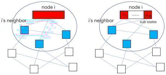
Figure 1.
The diagram shows the difference between diffKF (left) and DDKF (right). For any node i, represented by the red block, the blue block is i’s neighbors, and the diffusion network is shown as the blue line. Assuming that the state of node i can be divided into many sub-states, , DDKF sets different diffusion matrices for different sub-states.
2.2. Deep Diffusion Kalman Filter
Considering Equation (3), we assume that the system state variables can be divided into L sub-states , where and . The observation data are collected from the sub-states using the observation function ,
For convenience, we refer to Equation (3) to divide the observation function H into L parts, , where only the ith component is not part of the zero matrices. In order to provide a similar description using Algorithm 1, we denote the estimation of the state variables by sensor i as . Let denote the estimate of given the observations up to and including time . Let . We will now focus on describing the diffusion process of step 8.
In the DDKF method, it is desirable to use different diffusion matrices for updates in different states. Thus, for state , we denote the diffusion matrix as , which satisfies:
Let:
Referring to Equation (5), the deep diffusion process is described as follows:
and it has the same formula as Equation (6). Similarly, combined with Equation (7) and:
it can be found that:
and it has the same formula as Equation (8). Therefore, we can refer to the diffKF algorithm to put forward the DDKF, which is presented in Algorithm 2.
| Algorithm 2 Deep diffusion Kalman filter |
|
According to the Woodbury matrix identity, steps 3–7 in Algorithm 2 can be rewritten as follows:
If we denote , then .
The performance analysis of DDKF is listed in Section 3.1, and the experiment of DDKF is in Section 3.2.
2.3. Spiking Neuronal Network
2.3.1. Computational Neuron Model
The computational neuron model is generally a nonlinear operator ranging from a set of input synaptic spike trains to an output axon spike train that is described by three components: The subthreshold equation of the membrane potential, which describes the transformation from the synaptic currents of diverse synapses; the synaptic current equation, which describes the transformation from the input spike trains to the corresponding synaptic currents; and the threshold scheme, which provides the setup of the condition for triggering a spike by membrane potential.
Following [17], we consider the leakage integrate-and-fire (LIF) model as a neuron. A capacitance-voltage (CV) equation describes the membrane potential of neuron i when it is less than a given voltage threshold :
where is the capacitance of the neuron membrane, is the leakage conductance, is leakage voltage, is the synaptic current at the synapse type u of neuron i, and is the external stimulus from the environment; we set in this paper. Here, we consider at least four synapse types: AMPA, NMDA, , and [18].
Regarding the synapse model, We consider an exponentially temporal convolution that consists of this map:
Here, is the conductance of synapse type u of neuron i, is the voltage of synapse type u, is the time-scale constants of synapse type u of neuron i, is the connection weights from neuron j to I of synapse type u, is the Dirac delta function, and is the time point of the spike of neuron j.
When at , the neuron registers a spike at time point and the membrane potential is reset at during a refractory period:
After that, is governed by the CV equation again.
2.3.2. Network Topology
The whole cortex is divided into 90 regions of interest (ROIs) according to the Automated anatomical labeling atlas 3 (AAL3). The neuron number of each brain region (or ROI) is proportional to the density of gray matter of the high-resolution T1-weighted (T1W) MR images. Among them, the proportion of excitatory neurons is 80% and the proportion of inhibitory neurons is 20%.
The connection link between neurons is modeled as synapses, and there are four types of synapses, as mentioned in the previous section. For programming convenience, the in-degree of each neuron is set to be the same. Let be the adjacent matrix of synapse type u, where means that there is a link from neuron j to i and the conductance of this link is ; otherwise, . Each neuron has D neighbors and the network graph topology is generated by the following rule: each neuron randomly chooses a synaptic junction from excitatory neurons as excitatory synapses and inhibitory neurons as inhibitory synapses. Thus, the edge of each u synapse graph is .
Where the presynaptic neuron is located is dependent on the diffusion-weighted images (DWI). It is believed that the connections between brain regions are mainly excitatory connections, so the DWI reflects the connection density of excitatory synapses in brain regions. This paper has the following hypothesis: for each neuron, the ratio of excitatory synapse connections from the same brain region to the excitatory connections from other brain regions is 3:5, and the inhibitory synaptic connections are all from the same brain region.
The calculation iteration step of the entire model is 1 ms, and the mean of neuron activity spikes of each brain region is output as
We construct a cortex model with neurons and in-degree . The number of brain regions is .
2.4. BOLD Signal and Hemodynamical Model
Blood oxygenation level-dependent (BOLD) signal, detected using functional magnetic resonance imaging (fMRI), reflects the changes in deoxyhemoglobin that is driven by localized changes in brain blood flow and blood oxygenation, which are coupled with underlying neuronal activity through the process of neurovascular coupling. A useful mathematical model is the hemodynamical model, which takes the neural activity quantified by the spike rate of a pool of neurons and outputs the BOLD signal. Let be the time series of neural activity from Equation (20); the hemodynamical model can be generally written as . Here, g denotes the states related to blood volume and blood oxygen consumption. The BOLD signal is read as a function of g, i.e., . There are diverse hemodynamical models; herein, we introduce the Balloon–Windkessel model [19] as shown below:
Here, i is the label of the ROI, is the vasodilatory signal, is the blood inflow, is the blood volume, and is the deoxyhemoglobin content. , , , , , , , , , and are the constant parameters of the Balloon–Windkessel model. All parameters of the constant terms in the neuronal network model and hemodynamic model are set in Table 1.

Table 1.
Parameters in the neuronal network model and hemodynamic model.
2.5. Data Acquisition
All multimodal neuroimaging data were performed on a 3.0T MR scanner (Siemens Magnetom Prisma, Erlangen, Germany) at the Zhangjiang International Brain Imaging Center in Shanghai using a 64-channel head array coil.
High-resolution, T1-weighted (T1W) MR images were acquired using a 3D magnetization-prepared rapid gradient echo (3D-MPRAGE) sequence (repetition time (TR) = 3000 ms, echo time (TE) = 2.5 ms, inversion time (TI) = 1100 ms, field of view (FOV) = 256 mm, flip angle = , matrix size = , 240 sagittal slices, slice thickness = 0.8 mm, no gap).
Multi-shelled, multi-band diffusion-weighted images (DWIs) were acquired using a single-shot spin-echo planar imaging (EPI) sequence (monopolar scheme, repetition time (TR) = 3200 ms, echo time (TE) = 82 ms, matrix size = , voxel size = , multiband factor = 4, phase encoding: anterior to posterior) with two b-values of 1500 s/(30 diffusion directions) and 3000 s/(60 diffusion directions).
The resting-state fMRI was acquired using a gradient echo-planar imaging (EPI) sequence (repetition time (TR) = 800 ms, echo time (TE) = 37 ms, field of view (FOV) = 208 mm, flip angle = , matrix size = , voxel size = , multiband factor = 8).
3. Results
3.1. Theoretical Performance of the DDKF
In this section, we prove that when , the DDKF estimation of state x is unbiased and the variance converges. The proof is classical and can be referred to in the article [16].
The temporary state estimation error of sensor i is defined as , and the final state estimation error of sensor i is defined as . According to Equations (15) and (16), we have:
Because
thus,
Let
Then, the step 8 in Algorithm 2 can be rewritten as follows:
where .
Let
Then,
Furthermore,
Because for any . Thus, , which means that the DDKF estimation of the state variables is unbiased.
Let be the covariance of , ; then:
Assuming that the matrices do not change with t, which means that they are constant value matrices, the evolution matrix F is stable, which means that all eigenvalues of F have a modulus lengths of less than one, and in , the following limitations exist:
Then, there exists a constant such that , where is the unique solution to the following equation:
where
3.2. DDKF in the Toy Model
Before applying the DDKF method to assimilate large-scale neural networks, we first validated the effectiveness of the DDKF method through a small network toy model. Here, we use a simplified dynamic mean field model (DMF) [20] to calculate the global dynamics of the entire cerebral cortex. DMF consistently expresses the temporal evolution of collective activities of different excitatory and inhibitory neural populations. In the DMF model, the firing rate of each population depends on the input current entering the population. On the other hand, the input current depends on the firing rate of the respective populations. Therefore, the population firing rate can be determined automatically and consistently using a simplified system of coupled nonlinear differential equations that represent the population firing rate and input currents, respectively. The topology of the large-scale mean field model is generated according to the neuroanatomical connection DWI between these brain regions, which is connected by the structural connection matrix (SC).
The global brain dynamics are described by the following set of coupled nonlinear stochastic differential equations:
For the brain region i, represents the average firing rate of the excitatory neuron population, represents the average synaptic gating variable of the excitatory neuron population, represents the excitatory input current, and represents the connecting structure between brain area i and brain area j, which is generally derived from neural anatomical data. represents the activation function of the excitatory neuronal population, which maps the input current of the neuronal population to the firing rate, and are the constant parameters of this function. Correspondingly, the superscripts marked with I represent the relevant variables of the inhibitory neuron population. The parameters of the synaptic dynamics equation are set as . is the background input current, and are the parameters that regulate the background current of excitatory and inhibitory neuronal populations, respectively. is the synaptic current conductivity coefficient of NMDA, is the synaptic current conductivity coefficient of GABA, and G is the global coupling coefficient, which are used to regulate the neuronal population to maintain a lower level of spontaneous activity. represents the weight coefficient from the excitatory to the inhibitory neuronal population when connected to a neural network. Similarly, are defined as the weight coefficient. is the Gaussian noise with a variance of . We set up the model such that can be modified, and other parameter settings can be found in the article [21].
Then, based on the above model, we set the parameters in advance and then use DDKF to estimate . We compare the estimated values of model parameters and state values with the preset values to verify the effectiveness of our proposed method. To better compare the differences between the DDKF, DKF, and diffKF and to facilitate their application in brain network data assimilation, we set the number of brain regions in the DMF network to . At this point, the network connection matrix is , where elements are randomly sampled from according to a uniform distribution. The global coupling coefficient is , . The DMF model is nonlinear. We use the idea of ensemble Kalman filtering to calculate the covariance matrix, which generates simulated samples (particles) to simulate the system. By calculating the variance of the samples, we obtain the state covariance matrix of the system.
Assuming that our observation of the model is the average excitation rate of each brain region, the average excitation rate of the brain region i is:
Then, we estimate the parameters of each brain region in the model and the state variables based on the observation sequence. As mentioned in Section 2.1.1, is regarded following the equation . Thus, the state variables of DMF are .
In this paper, the sensor network required for the deep diffusion algorithm is set as follows: the sensor network is fully connected, and sensor i can only observe the average excitation rate of the brain region i. Finally, we use the average estimation of all sensors as the final estimate of the network state. When estimating the state of brain region r, we believe that the estimation performance of sensor r is better than that of other sensors. When information diffusion occurs, the proportion of sensor r should be higher than that of other sensors. Therefore, we design the following diffusion matrix :
Easy to verify, the diffusion matrix satisfies Equation (9), and we call the isolation coefficient of the deep diffusion algorithm. When , the weight of the sensor itself during the diffusion process is 0; that is, it completely adopts the system state estimated by other sensors. When , the weight of the sensor itself is 1; this means that the system state is only estimated by the sensor itself, and the algorithm is equivalent to the DKF method without neighbors. When , the weight of the sensor itself is the same as that of other sensors; that is, all sensors estimate the same system state after the diffusion process. At this time, the algorithm is equivalent to the diffKF method where each element of the diffusion matrix is 1. To gain a more intuitive understanding of the Algorithm 2, we have provided a detailed algorithm process under the diffusion matrix in Appendix B.
We note that the estimation error of the model parameters is:
and the assimilation error of the observation data is:
As shown in Figure 2, we demonstrate the impact of the value of on the data assimilation effect. It can be seen that under different values, the parameters and observation can ultimately be accurately estimated. More details can be found in Appendix B.
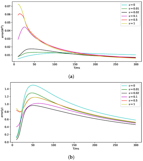
Notice that the definition of observation error represents the cumulative error, which results in the error seeming to be not too small. We define the real-time error as follows and calculate the errors under the different isolation coefficient , as shown in Table 2.
Table 2.
Real-time error under different isolation coefficients after DDKF data assimilation.
However, according to Figure 2a, a much larger leads to a much slower convergence speed. Thus, there is a balance between convergence speed and accuracy. We need to choose the proper isolation coefficient using prior knowledge to ensure system assimilation effectiveness.
3.3. Resting-State Twin Brain Assimilation
We use the deep diffusion Kalman filter method to estimate the state variables of the large-scale cortex model according to real resting-state brain BOLD signals. In this section, we assume that the AMPA synaptic conductance can be modified, and we add to the state variables. The real resting-state brain BOLD signals are a series of observation data from a total of time points, which were generated by the fMRI scanner with an observation frequency of 1.25 Hz. At any observation time, the dimension of the BOLD signals is the same as the number of brain regions in the cortex. The calculation iteration step of the neuronal network is still 1 ms, but to mimic the real BOLD signals series measured by fMRI, we set the observation function as a down-sampling process, recording every 800 ms interval.
Similarly, we compare the DKF, diffKF, and DDKF methods, which were evaluated by the assimilation error of the observation data and real-time error at the final time , shown in Table 3. The BOLD signals can be estimated well with a lower isolation coefficient and within a proper range; the larger the coefficient, the more accurate the estimation is. Excessive coefficients are not conducive to information exchange in sensor networks, making this method ineffective.
Table 3.
Observation error under different isolation coefficients after DDKF data assimilation.
Furthermore, we demonstrate the assimilation error of observation data during DDKF data assimilation, shown in Figure 3. Combined with Table 3, although smaller coefficients converge faster at the beginning, their final accuracy is not as good as larger coefficients.
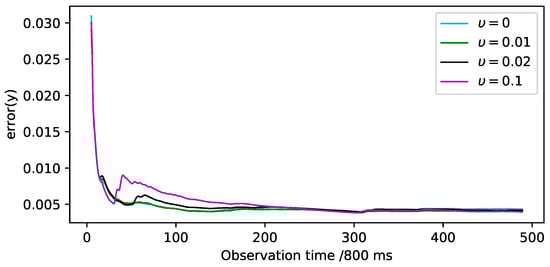
Figure 3.
The assimilation error of the real data, defined in Equation (32), are shown under different isolation coefficients.
Multi-scale brain connectivity refers to the physical and functional connectivity patterns between a group of brain units on multiple spatial scales. For large and complex systems such as the human brain, brain units can be defined as individual neurons, voxels, or macroscopic brain regions. The connectivity between these units can be further divided into the anatomical structural connectivity (SC) [22], functional connectivity (FC) [23] between their functional states, or effective connectivity of their inferred causal interactions (EC) [24]. Brain connectivity is the foundation of signal propagation in neural networks, making it crucial for understanding cognition and the flow of information and activity in the brain during health and disease.
The BOLD signal reflects the changes in activity and metabolism of different brain regions during fMRI brain imaging acquisition. It is believed that if the synchronization of BOLD signal changes in two brain regions is high, that is, if the synchronization of brain activity metabolism is high, then there should be a strong functional connection between these two brain locations. Usually, the FC matrix can be obtained by calculating the Pearson correlation coefficients of the BOLD signals of different brain regions [25]. Let denote the BOLD signal in brain region i as , then the ith row and jth column elements of the FC matrix are:
Based on the BOLD signal that we collected, we can draw an empirical functional connection matrix as shown in Figure 4. However, after data assimilation, we obtain a neural network system that can generate the BOLD signal, and we can observe the system by sampling neurons. According to the BOLD signals generated by the assimilated computational network, we can also calculate the assimilated functional connected matrix as shown in Figure 5. The correlation coefficient between the empirical and assimilated FC matrix is up to 98.42%. At the same time, some methods that adjust the global coupling parameter by exhaustive search can only achieve a correlation of around 50% [26,27], and this fully demonstrates that DA, as a data-simulating method, can effectively estimate BOLD signals and the FC matrix.
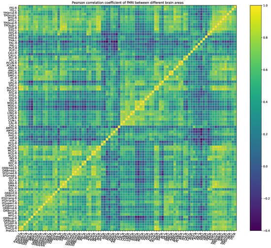
Figure 4.
Pearson correlation coefficient of the FMRI between different brain regions as calculated on real resting-state brain BOLD signals.
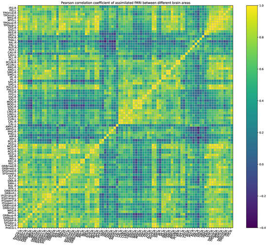
Figure 5.
Pearson correlation coefficient of the assimilated FMRI between different brain regions as calculated on real resting-state brain BOLD signals.
On the other hand, based on the activation of neurons in different brain regions per millisecond, we can also draw a connection matrix, as shown in Figure 6. The calculation method for the firing rate of different brain regions is to calculate the average firing rate of neurons in that brain region within 800 ms. It can be found that there is a certain similarity with the empirical FC matrix where the correlation coefficient is , and we believe that this statistical method can become a new tool for calculating functional connectivity matrices. Because we have achieved neuron-level modeling, we can study the process of synaptic transmission between brain regions or voxels or even between neurons, which is further helpful for us to understand the resting-state brain. Moreover, we can also study the mechanisms and treatment methods of brain diseases by conducting experiments on computational brain models without any moral or ethical issues.
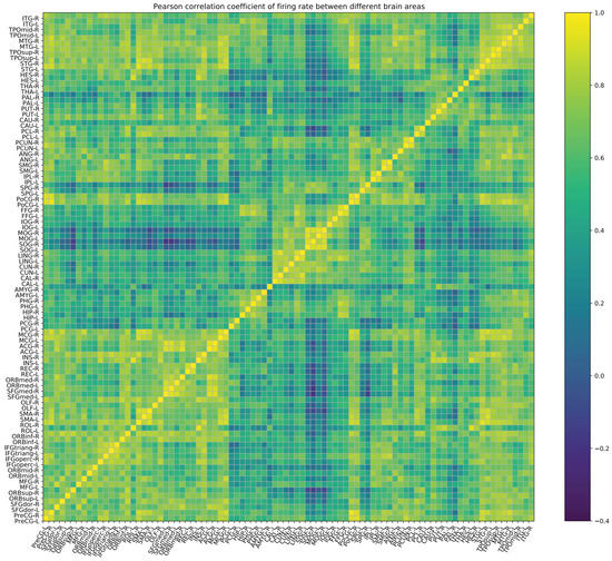
Figure 6.
Pearson correlation coefficient of the firing rate as calculated by collecting the mean firing rate of the brain regions in every 800 ms interval.
4. Conclusions and Discussion
In this paper, we put forward the deep diffusion Kalman filtering as a kind of data assimilation method. Essentially, DDKF is a general form of diffKF, and we have shown that the DDKF estimation of state variables is unbiased and that the variance converges using theoretical proof. In the toy model, we showed that DDKF can estimate the parameters and simulate the observation effectively, and the relative errors were less than 10%. Furthermore, using real human resting fMRI signals, we assimilated a computational brain network with the resting state brain, and the correlation was as high as 98.42%. We believe that the DDKF algorithm is an effective method for integrating large-scale neural network simulation with multimodal data.
However, DDKF adds information diffusion after DKF, which seems to increase the computational complexity and communication traffic compared with DKF. Actually, when we deal with neuroimaging data, the high dimension of data makes it difficult to reduce the computational complexity, especially for calculating the inverse of high-dimensional matrices. If we regard the high-dimensional observation data as a combination of multiple low-dimensional observation data collected by sensors, the inverse of the high-dimensional matrix becomes the inverse of multiple low-dimensional matrices, which greatly reduces the computational complexity. In this case, introducing the information diffusion only linearly increases the computational complexity but brings significant results.
The sensor network in this paper was set as a fully connected matrix, which was because we used a personal computer to realize the cortex neuronal network. As the scale of computational networks increases, modern supercomputers consisting of clusters of computing nodes have been used to assign neurons and synapses to multiple computer nodes for parallel processing [28]. The construction of sensor networks needs to consider the real physical connection topology between computing nodes. Meanwhile, when simulating human brain neural networks, DTI should be considered as the basis for communication between ROIs or voxels. The communication traffic between nodes has become a limitation for efficient simulations, which requires careful design. We believe that DKF and DDKF will play more important roles in this situation.
Although the neuron number of the cortex model network is up to 10 million, the parameters of the neurons are the same, which means that the network is homogeneous. Continuing to increase the number of neurons is only a consumption of computational resources and maybe has no essential improvement on the dynamic behavior.Heterogeneous networks need to be considered, and the estimation of network parameters is also important. Assuming that the parameters of the neurons and synapses are inhomogeneous but are independently and identically distributed from certain distributions with unknown hyperparameters, hierarchical data assimilation (HDA) [29] serves as an effective estimation framework. DDKF can also be combined with HDA, and further work can refer to [30].
Author Contributions
Conceptualization, W.L.; methodology, W.Z. and W.L.; software, W.Z.; validation, W.Z. and W.L.; formal analysis, W.Z.; investigation, W.Z.; resources, W.L.; data curation, W.L.; writing—original draft preparation, W.Z.; writing—review and editing, W.L.; visualization, W.Z.; supervision, W.L.; project administration, W.L.; funding acquisition, W.L. All authors have read and agreed to the published version of the manuscript.
Funding
This research was funded by the National Key R&D Program of China (No. 2018AAA0100303), National Natural Science Foundation of China (No. 62072111), Shanghai Municipal Science and Technology Major Project (No. 2018SHZDZX01), and Zhangjiang Lab.
Data Availability Statement
Data are available upon request due to privacy restrictions. The data presented in this study are available upon request from the corresponding author. The data are not publicly available due to being collected by our own laboratory.
Conflicts of Interest
The authors declare no conflict of interest.
Abbreviations
The following abbreviations are used in this manuscript:
| KF | Kalman filter |
| DKF | Distributed Kalman filter |
| diffKF | Diffusion Kalman filter |
| DDKF | Deep diffusion Kalman filter |
| DA | Data assimilation |
| HDA | Hierarchical data assimilation |
| BOLD | Blood oxygen level-dependent |
| fMRI | Functional magnetic resonance imaging |
| LIF | Leakage integrate-and-fire |
| CV | Capacitance-voltage equation |
| DWI | Diffusion-weighted image |
| AMPA | -amino-3-hydroxy-5-methyl-4-isoxazole propionic acid receptor |
| NMDA | N-methyl-D-aspartate receptor |
| -Aminobutyric acid sub-type A receptors | |
| G-protein-coupled receptors |
Appendix A. Overview of Data Assimilation
Notice that the stochastic dynamical system using Equations (1) and (2) is in discrete form, but the function F can be the solution operator for an ordinary differential equation (ODE) of the form:
Assuming that the solution exists for all , then the one-parameter semigroup of operators , parameterized by time , is well defined. In this situation, we assume that is the solution operator over time units; then, we have .
When estimating the state variables x, according to the different observation data available, DA is subdivided into two prominent families of methodology, the family of offline smoothing methods and the family of online filtering algorithms. Smoothing methods estimate state variables after gathering all observation data , while filtering methods estimate state variables according to the observation data before the current moment . From the perspective of Bayesian conditional probability, smoothing methods estimate the posterior probability distribution and filtering methods estimate . In this paper, we focus on filtering methods, and more details on smoothing methods can be referred to in [12].
If we assume that the posterior probability distribution has been estimated at any time t, then for , the filter methods provide a framework to estimate . That is, using to estimate is called prediction step, and using to estimate is called the analysis step.
In the prediction steps, according to the Markov property, we have
Thus, the prediction step is to find a map from to . Similarly, in the analysis steps,
Thus, the analysis step is to find a map from to .
Appendix B. Details of Toy Model
For the toy model using Equations (23)–(28), the number of brain regions is . Let . Thus, the DMF state X can be divided into 90 parts , where . The observation of is . Next, we will provide a detailed introduction to the algorithm process. Taking the first brain region as an example, the estimation of sub-state is more accurate according to observation . Thus, if we assume that there is a sensor network, the sensor that only observes the first brain region could estimate the sub-state more accurately. Therefore, other sensors that estimate the sub-state should refer more to the first sensor. At this time, the first row of diffusion matrix of sub-state , which refers to the diffusion rate from other sensors to the first sensor, is set to . However, for sub-state , the first row of diffusion matrix , which refers to the diffusion rate from other sensors to the first sensor, is set to because we assume that the sensor that only observes the second brain region could estimate sub-state more accurately.
Returning to Algorithm 2, let us use to represent the first sub-state of estimation of sensor i and use to present the first sub-state of estimation . Under the circumstances, step 8 means:
If we use to represent the first sub-state of estimation of sensor i, then:
Regarding the details of the data assimilation in the toy model, for the convenience of drawing, we set and show the details of the small-scale DMF model as follows. First, we set for all three brain regions, then simulated the DMF model and drew the states as follows.

Figure A1.
The excitatory input current in the DMF model.

Figure A2.
The inhibitory input current in the DMF model.

Figure A3.
The average synaptic gating variable of the excitatory neuron population in DMF.

Figure A4.
The average synaptic gating variable of the inhibitory neuron population in DMF.

Figure A5.
The average firing rate of the excitatory neuron population in DMF.

Figure A6.
The average firing rate of the inhibitory neuron population in DMF.
Meanwhile, the observation of the three brain regions is shown in Figure A7.

Figure A7.
The observation of the three brain regions in the DMF model.
Then, we use DDKF to estimate the parameters and simulate the observation. Here, we only show the experiment results on in the following figures. The red lines are the true value or baseline, the blue lines are the estimation of parameters or observation, and the blue shading represents the variance of estimation.

Figure A8.
The parameter estimation of brain region 1.

Figure A9.
The parameter estimation of brain region 2.

Figure A10.
The parameter estimation of brain region 3.

Figure A11.
The observation simulation of brain region 1.

Figure A12.
The observation simulation of brain region 2.

Figure A13.
The observation simulation of brain region 3.
References
- Herculano-Houzel, S. The human brain in numbers: A linearly scaled-up primate brain. Front. Hum. Neurosci. 2009, 3, 31. [Google Scholar] [CrossRef] [PubMed]
- Markram, H. The Blue Brain Project. Nat. Rev. Neurosci. 2006, 7, 153–160. [Google Scholar] [CrossRef] [PubMed]
- Amunts, K.; Ebell, C.; Muller, J.; Telefont, M.; Knoll, A.; Lippert, T. The Human Brain Project: Creating a European Research Infrastructure to Decode the Human Brain. Neuron 2016, 92, 574–581. [Google Scholar] [CrossRef] [PubMed]
- Leon, P.S.; Knock, S.A.; Woodman, M.M.; Domide, L.; Mersmann, J.; McIntosh, A.R.; Jirsa, V. The Virtual Brain: A simulator of primate brain network dynamics. Front. Neuroinform. 2013, 7, 10. [Google Scholar] [CrossRef]
- Michel, C.M.; Murray, M.M. Towards the utilization of EEG as a brain imaging tool. NeuroImage 2012, 61, 371–385. [Google Scholar] [CrossRef] [PubMed]
- Boto, E.; Holmes, N.; Leggett, J.; Roberts, G.; Shah, V.; Meyer, S.S.; Muñoz, L.D.; Mullinger, K.J.; Tierney, T.M.; Bestmann, S.; et al. Moving magnetoencephalography towards real-world applications with a wearable system. Nature 2018, 555, 657–661. [Google Scholar] [CrossRef]
- Friston, K.J.; Kahan, J.; Razi, A.; Stephan, K.E.; Sporns, O. On nodes and modes in resting state fMRI. NeuroImage 2014, 99, 533–547. [Google Scholar] [CrossRef]
- van den Heuvel, M.P.; Mandl, R.C.; Kahn, R.S.; Pol, H.E.H. Functionally linked resting-state networks reflect the underlying structural connectivity architecture of the human brain. Hum. Brain Mapp. 2009, 30, 3127–3141. [Google Scholar] [CrossRef]
- Rektorova, I. Resting-State Networks in Alzheimer Disease and Parkinson Disease. Neurodegener. Dis. 2013, 13, 186–188. [Google Scholar] [CrossRef]
- Eibern, H.; Schmidt, H. A four-dimensional variational chemistry data assimilation scheme for Eulerian chemistry transport modeling. J. Geophys. Res. Atmos. 1999, 104, 18583–18598. [Google Scholar] [CrossRef]
- Hoteit, I.; Pham, D.T.; Triantafyllou, G.; Korres, G. A New Approximate Solution of the Optimal Nonlinear Filter for Data Assimilation in Meteorology and Oceanography. Mon. Weather. Rev. 2008, 136, 317–334. [Google Scholar] [CrossRef]
- Law, K.; Stuart, A.; Zygalakis, K. Data Assimilation; Springer: Berlin/Heidelberg, Germany, 2015; Volume 62. [Google Scholar] [CrossRef]
- Abarbanel, H.D.I.; Rozdeba, P.J.; Shirman, S. Machine Learning: Deepest Learning as Statistical Data Assimilation Problems. Neural Comput. 2018, 30, 2025–2055. [Google Scholar] [CrossRef] [PubMed]
- Kalman, R.E. A New Approach to Linear Filtering and Prediction Problems. J. Basic Eng. 1960, 82, 35–45. [Google Scholar] [CrossRef]
- Mahmoud, M.S.; Khalid, H.M. Distributed Kalman filtering: A bibliographic review. IET Control Theory Appl. 2013, 7, 483–501. [Google Scholar] [CrossRef]
- Cattivelli, F.S.; Sayed, A.H. Diffusion Strategies for Distributed Kalman Filtering and Smoothing. IEEE Trans. Autom. Control 2010, 55, 2069–2084. [Google Scholar] [CrossRef]
- Brunel, N.; Wang, X.J. Effects of neuromodulation in a cortical network model of object working memory dominated by recurrent inhibition. J. Comput. Neurosci. 2001, 11, 63–85. [Google Scholar] [CrossRef]
- Yang, G.R.; Murray, J.D.; Wang, X.J. A dendritic disinhibitory circuit mechanism for pathway-specific gating. Nat. Commun. 2016, 7, 12815. [Google Scholar] [CrossRef]
- Friston, K.; Mechelli, A.; Turner, R.; Price, C. Nonlinear Responses in fMRI: The Balloon Model, Volterra Kernels, and Other Hemodynamics. NeuroImage 2000, 12, 466–477. [Google Scholar] [CrossRef]
- Wong, K.F.; Wang, X.J. A Recurrent Network Mechanism of Time Integration in Perceptual Decisions. J. Neurosci. 2006, 26, 1314–1328. [Google Scholar] [CrossRef]
- Deco, G.; Ponce-Alvarez, A.; Hagmann, P.; Romani, G.L.; Mantini, D.; Corbetta, M. How Local Excitation-Inhibition Ratio Impacts the Whole Brain Dynamics. J. Neurosci. 2014, 34, 7886–7898. [Google Scholar] [CrossRef]
- Hagmann, P.; Cammoun, L.; Gigandet, X.; Gerhard, S.; Grant, P.E.; Wedeen, V.; Meuli, R.; Thiran, J.P.; Honey, C.J.; Sporns, O. MR connectomics: Principles and challenges. J. Neurosci. Methods 2010, 194, 34–45. [Google Scholar] [CrossRef] [PubMed]
- Trapnell, C.; Cacchiarelli, D.; Grimsby, J.; Pokharel, P.; Li, S.; Morse, M.; Lennon, N.J.; Livak, K.J.; Mikkelsen, T.S.; Rinn, J.L. The dynamics and regulators of cell fate decisions are revealed by pseudotemporal ordering of single cells. Nat. Biotechnol. 2014, 32, 381–386. [Google Scholar] [CrossRef]
- Friston, K.J. Functional and effective connectivity in neuroimaging: A synthesis. Hum. Brain Mapp. 1994, 2, 56–78. [Google Scholar] [CrossRef]
- Friston, K.J.; Frith, C.D.; Liddle, P.F.; Frackowiak, R.S.J. Functional Connectivity: The Principal-Component Analysis of Large (PET) Data Sets. J. Cereb. Blood Flow Metab. 1993, 13, 5–14. [Google Scholar] [CrossRef] [PubMed]
- Deco, G.; Jirsa, V.K. Ongoing Cortical Activity at Rest: Criticality, Multistability, and Ghost Attractors. J. Neurosci. 2012, 32, 3366–3375. [Google Scholar] [CrossRef]
- Deco, G.; Cabral, J.; Saenger, V.M.; Boly, M.; Tagliazucchi, E.; Laufs, H.; Someren, E.V.; Jobst, B.; Stevner, A.; Kringelbach, M.L. Perturbation of whole-brain dynamics in silico reveals mechanistic differences between brain states. NeuroImage 2018, 169, 46–56. [Google Scholar] [CrossRef]
- Igarashi, J.; Yamaura, H.; Yamazaki, T. Large-Scale Simulation of a Layered Cortical Sheet of Spiking Network Model Using a Tile Partitioning Method. Front. Neuroinform. 2019, 13, 71. [Google Scholar] [CrossRef]
- Zhang, W.; Chen, B.; Feng, J.; Lu, W. On a framework of data assimilation for neuronal networks. arXiv 2022, arXiv:2206.02986. [Google Scholar] [CrossRef]
- Lu, W.; Zheng, Q.; Xu, N.; Feng, J.; DTB Consortium. The human digital twin brain in the resting state and in action. arXiv 2022, arXiv:2211.15963. [Google Scholar] [CrossRef]
Disclaimer/Publisher’s Note: The statements, opinions and data contained in all publications are solely those of the individual author(s) and contributor(s) and not of MDPI and/or the editor(s). MDPI and/or the editor(s) disclaim responsibility for any injury to people or property resulting from any ideas, methods, instructions or products referred to in the content. |
© 2023 by the authors. Licensee MDPI, Basel, Switzerland. This article is an open access article distributed under the terms and conditions of the Creative Commons Attribution (CC BY) license (https://creativecommons.org/licenses/by/4.0/).