Omni-Domain Feature Extraction Method for Gait Recognition

Abstract

As a biological feature with strong spatio-temporal correlation, the current difficulty of gait recognition lies in the interference of covariates (viewpoint, clothing, etc.) in feature extraction. In order to weaken the influence of extrinsic variable changes, we propose an interval frame sampling method to capture more information about joint dynamic changes, and an Omni-Domain Feature Extraction Network. The Omni-Domain Feature Extraction Network consists of three main modules: (1) Temporal-Sensitive Feature Extractor: injects key gait temporal information into shallow spatial features to improve spatio-temporal correlation. (2) Dynamic Motion Capture: extracts temporal features of different motion and assign weights adaptively. (3) Omni-Domain Feature Balance Module: balances fine-grained spatio-temporal features, highlight decisive spatio-temporal features. Extensive experiments were conducted on two commonly used public gait datasets, showing that our method has good performance and generalization ability. In CASIA-B, we achieved an average rank-1 accuracy of 94.2% under three walking conditions. In OU-MVLP, we achieved a rank-1 accuracy of 90.5%.

1. Introduction

As an emerging biometric technology, it refers to the use of video of human gait, processed by computer vision methods, to recognize or to identify persons based on their body shape and walking styles [1].

It adopts a passive mode of acquiring biological information from a distance, so compared with other traditional biometric technologies (such as face recognition, fingerprint recognition, iris recognition, etc.), gait recognition has the advantages of being non-intrusive, difficult to hide, and hard to imitate. It has broad application prospects in video surveillance, security protection, suspect tracking. At present, most of the gait recognition methods based on deep learning have two main problems:

1. It is self-evident that temporal features play an important role in gait recognition. The current methods are based on the original sequence to mine temporal information. As shown in the Figure 1, we believe that reorganizing the gait sequence by using an interval frame sampling method can capture more information about joint dynamic changes. Therefore, we propose an interval frame sampling method, which performs interval sampling on the original gait frame sequence to obtain multiple interval sub-sequences, thereby enhance the representation ability of features.

2. At present, the main problem in gait recognition based on visual information is that it is difficult to extract key discriminative features from multiple perspectives and under the interference of complex variables. The quality of feature extraction determines whether the expression of the identity of the gait subject is correct. This puts forward higher requirements for the design of the feature extraction method. Compared with the static recognition of general biometric technologies such as face recognition and fingerprint recognition, gait recognition contains abundant dynamic features. Dynamic features contain temporal information, and temporal information and spatial information are closely combined to form the motion pattern of gait. Most of the current state-of-the-art gait recognition methods roughly split the supposedly closely connected spatio-temporal feature extraction process into two separate feature extraction modules. In this process, key spatio-temporal information will lost and make the spatio-temporal information mismatch. In some complex scenes, the representation ability of the final features will be reduced. Combining the interval frame sampling of the first point, we design an Omni-Domain Feature Extraction Network for gait recognition.

This method injects prominent temporal information into the extraction process of shallow spatial features to improve the discrimination ability of features. Further, through the dynamic motion capture, a range of temporal information of different motion is obtained, and finally, the temporal information and spatial information are balanced through the Omni-Domain Feature Balance Module to obtain the final feature representation.

In summary, the main contributions of this paper are as follows:

1. We propose a sequence reorganization method of interval frames, which complements the original frame sequence and enhances the richness of temporal information.

2. Combining interval frame sampling, a Temporal-Sensitive Feature Extractor for gait recognition is proposed to improve the representation ability of shallow spatial features by injecting temporal information into frame-level feature extraction.

3. Dynamic Motion Capture is proposed to extract temporal features of different motion and assign weights adaptively.

4. Omni-Domain Feature Balance Module, which further refines the temporal features of different motion and integrates the spatio-temporal features, highlights the decisive features.

5. Through a large number of experiments, it is proved that our proposed method has achieved a competitive results compared with the state-of-the-art method.

2. Related Work

2.1. Model-Based

Model-based gait recognition concerns identification using an underlying mathematical construct (s) representing the discriminatory gait characteristics (be they static or dynamic), with a set of parameters and a set of logical and quantitative relationships between them [2]. The model-based method [3,4,5,6,7,8,9,10] can be divided into two steps. The first step is to mathematically model the human body structure and movement. The second step is to extract features based on the bone key point map obtained from the modeling results.

2.1.1. Pose Estimation

PoseGait [3,4] use a pre-trained model of multi-person 2D pose estimation (containing 18 connection points) model [11] to obtain human pose information. In addition, in order to improve the robustness of the model to appearance variables, it normalizes the human pose and manually selects LHip, RKnee, Kankle, Lhip, LKnee, and Lankle: six connection points as the input gait features. Ref. [6] use HRNet [12] pre-trained by COCO dataset [13] as a 2D human body pose estimator, and then, through image enhancement methods such as flip and mirror to obtain the input of the network and add Gaussian noise at the connection points to improve the robustness of the network. Ref. [7] use the pre-training models of OpenPose [14] and AlphaPose [15] to obtain human body posture information. It uses three dynamic modes (natural connection, temporal correlation, and symmetric interaction) to operate on human body posture information and improve the expression ability of features.

2.1.2. Feature Extraction

PoseGait [3,4] proposed pose-based temporal–spatial network (PTSN), which consists of two branches, Long Short-Term Memory (LSTM) network branch and Convolutional Neural Network (CNN) branch; the former is used to extract dynamic temporal features from gait sequences; the latter is used to extract static spatial features from gait frames; and finally, the combination of static and dynamic features is used to obtain the final feature representation. The feature extraction network in [6] consists of multiple Res-Graph Concolutional Networks (ResGCN) [16]. Specifically, a graph convolution is followed by a 2D convolution in the time domain, and residual connections are used as Bottleneck blocks. The three dynamic pattern features obtained by preprocessing are input into the designed hyper feature network as a hierarchical deep convolutional neural network, and its output is the multi-level features, including dynamic features at high level, structured features at intermediate level, static features at low level. The three features are mixed by global average pooling (GAP).

2.2. Appearence-Based

The appercence-based methods [17,18,19,20,21,22,23,24,25,26,27] directly extract features from the original gait silhouette. Most of the existing methods based on convolution neural network adopt a three-step network form; Firstly, extract the spatial frame-level features pertinently, and further mine the potential temporal information between frames. Finally, the feature fusion module is used to fuse temporal and spatial features to obtain fine-grained and discriminative spatio-temporal features.

2.2.1. Spatial Feature Extraction

At present, there are three main ways to extract spatial frame-level features: (1) [17,18,19,20,21,22,23,24] directly extracted features from the input frame-level images through 2D convolution without any temporal operation. (2) In [18], the frame-level feature is extracted through 3D convolution operation. However, due to the complex operation of 3D convolution, it is difficult to converge, and requires more computational resources, so the obtained spatial frame-level feature can not represent the gait pattern well. (3) The idea adopted by [23,24] is to divide the human gait contour into different parts so as to apply convolution operation to obtain fine-grained frame-level features and improve the representation ability of frame-level features.

2.2.2. Temporal Representation

GaitPart [23] uses a module called the Micro-Motion Template Builder to map fine-grained frame-level features into feature vectors sufficient to capture subtle actions. It improves the distinguishing ability of features by extracting short-range temporal features from frame-level information and fusing them with spatial features. GaitGL [18] use the Local Temporal Aggregation (LTA) component to aggregate temporal information on the basis of preserving spatial information. CSTL [22,28] operates frame-level features on the temporal dimension through Multi-Scale Temporal Extraction to obtain features of three different scales (Frame-Level, Short-Term, Long-Term), which enriches the temporal information and improves the representation ability of features.

2.2.3. Spatio-Temporal Feature Fusion

In [18], the Global and Local Feature Extractor (GLFE) module is used to fuse global and local features, and the final feature representation is obtained through the mapping of Temporal Pooling and GeM Pooling. CSTL [22] input the three temporal features of different scales into Adaptive Temporal Aggregation (ATA) and Salient Spatial Feature Learning (SSFL), respectively. The ATA module can exchange the temporal information of different scales and enrich the temporal representation ability of features. SSFL further extracts prominent spatial features to eliminate possible overlap in behavioral features. Finally, the fusion of features is completed through the connection operation.

3. Materials and Methods

3.1. Overview

As shown in Figure 2, the sequence of gait silhouette will be input into our proposed network. To begin with, as the first feature extractor in our model, the silhouette contain N frames will be sent to Temporal-Sensitive Feature Extractor (TSFE) to obtain the shallow spatial feature $F_i$.

$$F_i=TSFE\left(x_i\right)$$

(1)

where i denotes the index of frame in gait sequence ($i\in 1,2,...,N$).

Then, in order to take out redundant information and reduce feature dimensions, shallow spatial feature $F_i$ will be entered into Horizontal Pooling (HP) layer. Here, we choose the maximum value function as the horizontal pooling strategy; then, the compressed feature $H_i$ are obtained.

$$H_i=HP\left(F_i\right)$$

(2)

At the same time, we use our proposed plug-and-play strategy here, Interval Sampling Strategy, to reorganize and enhance frame-level features to capture more dynamics over time. This process is expressed by the formula:

$$S_i=IntervalSampling\left(H_i\right)$$

(3)

In the next step, enhanced features after reorganization feature $S_i$ are injected into the module through Dynamic Motion Capture (DMC); temporal features of different motion $D_i$ can be described as:

$$D_i=DMC\left(S_i\right)$$

(4)

At last, the final feature representation $Y_i$ will be obtained through the Omni-Domain Feature Balance Module (ODB)

$$Y_i=ODB\left(D_i\right)$$

(5)

Through the Separate Fully Connected (FC) layer, the feature objective for training is as follows:

$$X_i=FC\left(Y_i\right)$$

(6)

3.2. Temporal-Sensitive Feature Extractor

3.2.1. Discussion

Using simple 2D convolution as a method of shallow spatial feature extraction, the main problems are: (1) Insufficient spatial awareness, limited by the size of the convolution kernel, it can only focus on the spatial information of the local area, and too large convolution kernel will increase the number of parameters. (2) Temporal clues are not used. As a biometric technology that contains rich temporal and spatial clues, the primary characteristic of gait recognition is the rich clues available in time domain and space domain. However, using simple 2D convolution to extract shallow features loses information in the temporal dimension. The use of 3D convolution as a shallow feature extraction method will solve the problem of temporal information loss, but the problem of insufficient spatial information perception still exists, and the training process of 3D convolution is difficult to converge due to its complex operation mechanism. Therefore, in order to solve the above problems, we propose a temporal-sensitive feature extractor. The main contributions are: (1) In order to enhance the spatial perception ability, we added the dilation operation, which can expand the perception range of the convolution kernel without increasing the amount of parameters, and accumulate the perception range of the kernel, so as to obtain richer spatio-temporal information. (2) In the process of spatial feature extraction, by injecting temporal information, the relevance of spatio-temporal information is improved and the discrimination ability of features is increased.

3.2.2. Operation

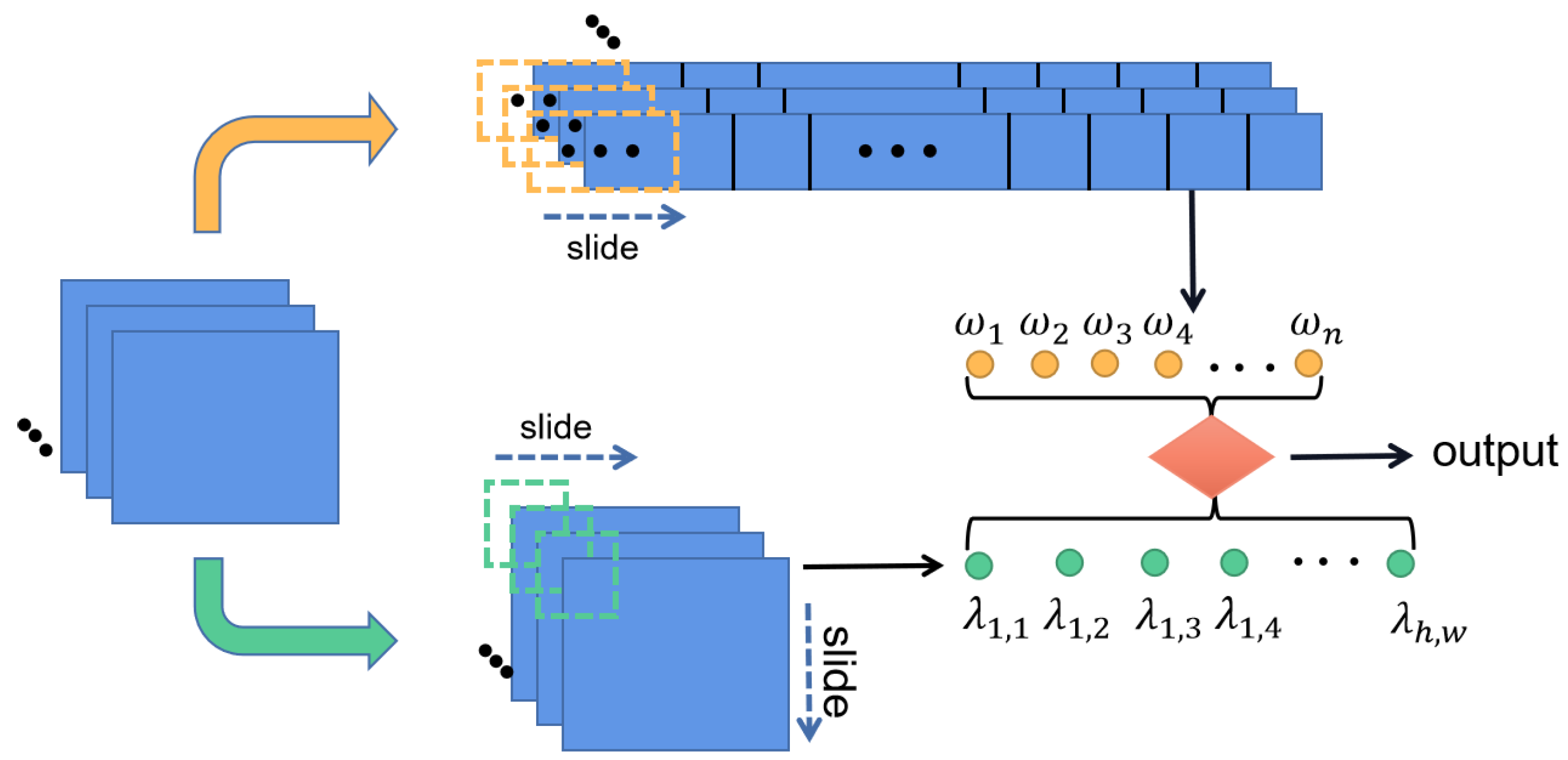
As shown in Figure 3, the temporal-sensitive feature extractor contains two parallel branches, a 2D dilated convolution for spatial feature extraction, and a 1D dilated convolution in time-domain to mine temporal clues. The spatial feature extraction process can be described by the following formula, It should be noted that $\lambda$ represents the parameter for each 1D convolution kernel (assuming the size of the convolution kernel is n), and $\omega$ represents for each 2D convolution (assuming the size of the convolution kernel is $h\ast w$). For qualitative analysis, we use 1 channel of one gait frame for parameter description: the specific parametric representation of a 2D convolution for spatial feature extraction is as follows:

$$s=({\lambda }_{1,1}+...+{\lambda }_{h,w})\ast x$$

(7)

Temporal clues can be expressed by the following formula:

$$t=({\omega }_1+...+{\omega }_n)\ast x$$

(8)

The schematic diagram of the specific dilated convolution is shown in the Figure 4, from which we can see that compared with the traditional convolution kernel, under the premise of the same parameter settings, the dilated convolution has a larger receptive field, so it can capture abundant information. For the spatial information and spatio-temporal cues obtained by the parallel structure, we combine them in the following way. The spatial features and the temporal cues extracted by each layer are combined in the form of dot products. At the same time, in order to highlight the role of shallow spatial features, the features with temporal clues and without temporal clues are added to obtain the output of the layer. The formula is as follows:

$$outpu{t}_{tsfe}=s\ast t+s=\left(({\lambda }_{1,1}+...+{\lambda }_{h,w})({\omega }_1+...+{\omega }_n+1)\right))\ast x$$

(9)

3.3. Dynamic Motion Capture

3.3.1. Discussion

After the feature extraction process, the traditional gait recognition methods only pay attention to the extraction of the global feature or the extraction of local features, while ignoring the coordination between joints and the subtle feature changes inside the joints. Therefore, in this paper, we propose a Dynamic Motion Capture (DMC), which can extract motion features of different scales. Specifically, we use four types of features, namely, Macro-Motion, Meso-Motion, Micro-Motion, and Sub-Motion. Among them, Macro-Motion is used to capture the global motion characteristics of the human body. Meso-Motion is a coordinated change between different joint parts of the human body. Micro-Motion is a subtle change inside the joints of the human body. Sub-Motion is an extremely small movement in the gait cycle.

3.3.2. Operation

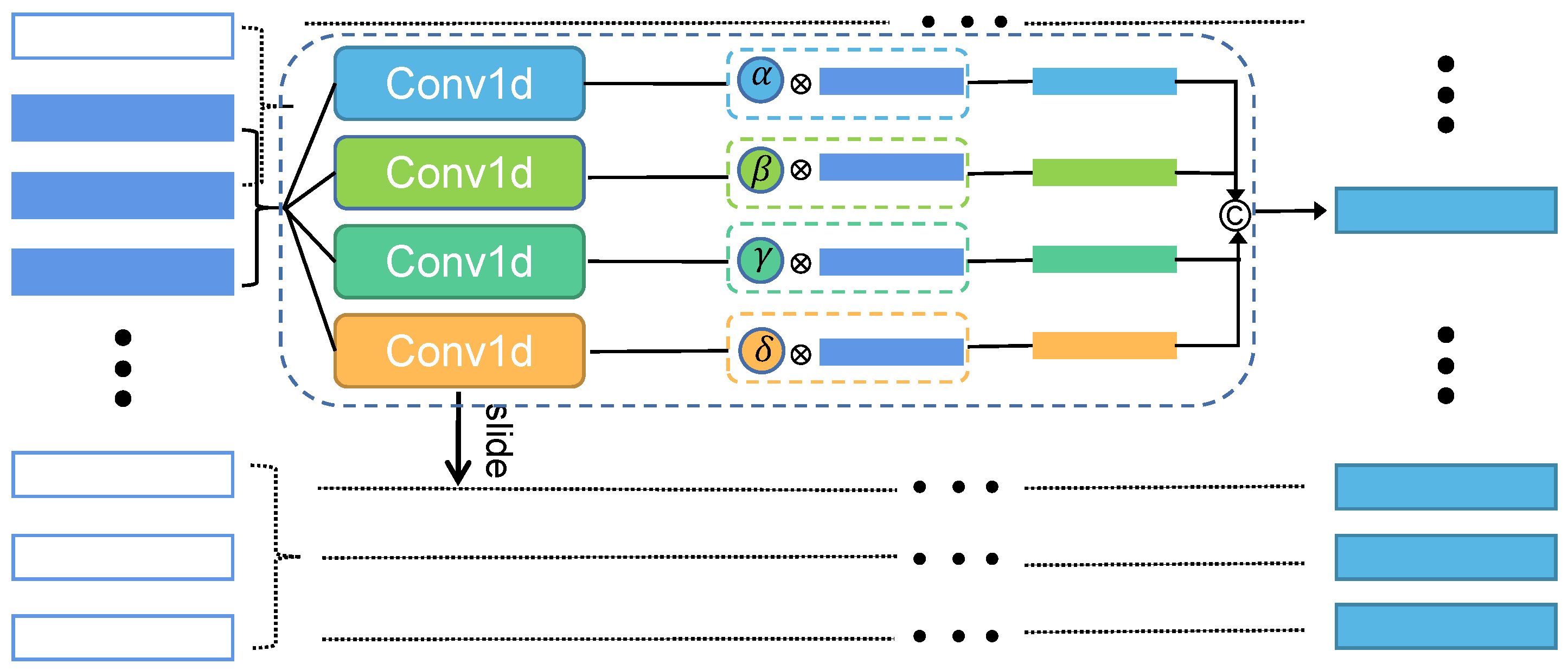
Convolution is an efficient feature extraction method, and the receptive field that changes with the size of the convolution kernel is extremely important for the effect of feature extraction. Therefore, as shown in Figure 5, we use 1D convolution operations with different kernels to mine multi-scale information of gait, and obtain temporal characteristics of different scales through receptive fields of different sizes. For Macro-Motion, we focus on the global motion characteristics of the human body, so we use a larger convolution kernel to model it. Meso-Motion pays more attention to the coordinated motion features between different body parts; therefore, we reduce the size of the convolution kernel. Micro-Motion uses a smaller convolution kernel for subtle changes between body parts. Sub-Motion uses a fully connected layer to model fine-grained information. Finally, the fused features are obtained through the concatenation operation. The above process can be represented by the following parameterized formula. (different letters are represented by parameters with different convolution kernel sizes.)

$$y=(({\alpha }_1+...+{\alpha }_m)Ⓒ({\beta }_1+...+{\beta }_n)Ⓒ({\gamma }_1+...+{\gamma }_p)Ⓒ({\sigma }_1+...+{\sigma }_q))\ast x$$

(10)

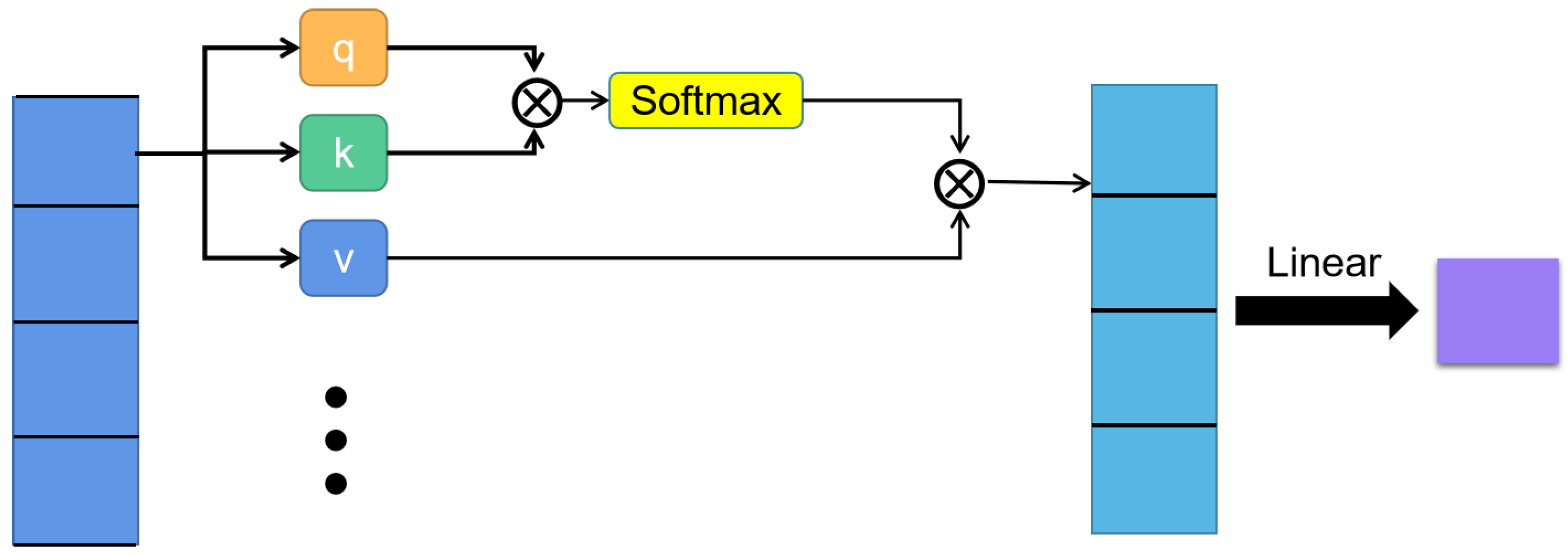
At the same time, we believe that features of different scales will play different roles in feature discrimination, so we decided to use self-attention mechanism to give different weights to motion of different scales. As shown in Figure 6, different motions are sent into the self-attention module, the features with different motion of multi-head self-attention mechanism will be given different weights, which will make the features more representative of the correlation on the motion scale and highlight the representative ability of the features.

Query $q\in R^{d_q}$, $k\in R^{d_k}$, value $v\in R_v^d$, the attention head could be formulated as:

$$h_i=f(W_i^{\left(q\right)}\ast q,W_i^{\left(k\right)}\ast k,W_i^{\left(v\right)}\ast v)\in R^{p_v}$$

(11)

where f is scaled dot-product attention, $W_i^{\left(q\right)}\in R^{p_q\ast d_q}$, $W_i^{\left(k\right)}\in R^{p_k\ast d_k}$, $W_i^{\left(v\right)}\in R^{p_v\ast d_v}$.

Through a linear layer, the output will be obtained ($W_o\in R^{p_o\ast h{p}_v}$, Ⓒ represents concatenation):

$$ouput=W_o\ast (h_1Ⓒ...Ⓒh_n)$$

(12)

3.4. Omni-Domain Feature Balance Module

3.4.1. Discussion

After the adaptive multi-scale temporal information injection module, feature representations with tight spatio-temporal connections are obtained. However, after the above operations on temporal and spatial features, the expression ability of the features we obtained improved, but the prominent features of space and the rich features of temporal information need to be further balanced to achieve better discrimination ability. Therefore, we propose an Omni-Domain Feature Balance Module to balance and integrate the rich information contained in space and time domain.

3.4.2. Operation

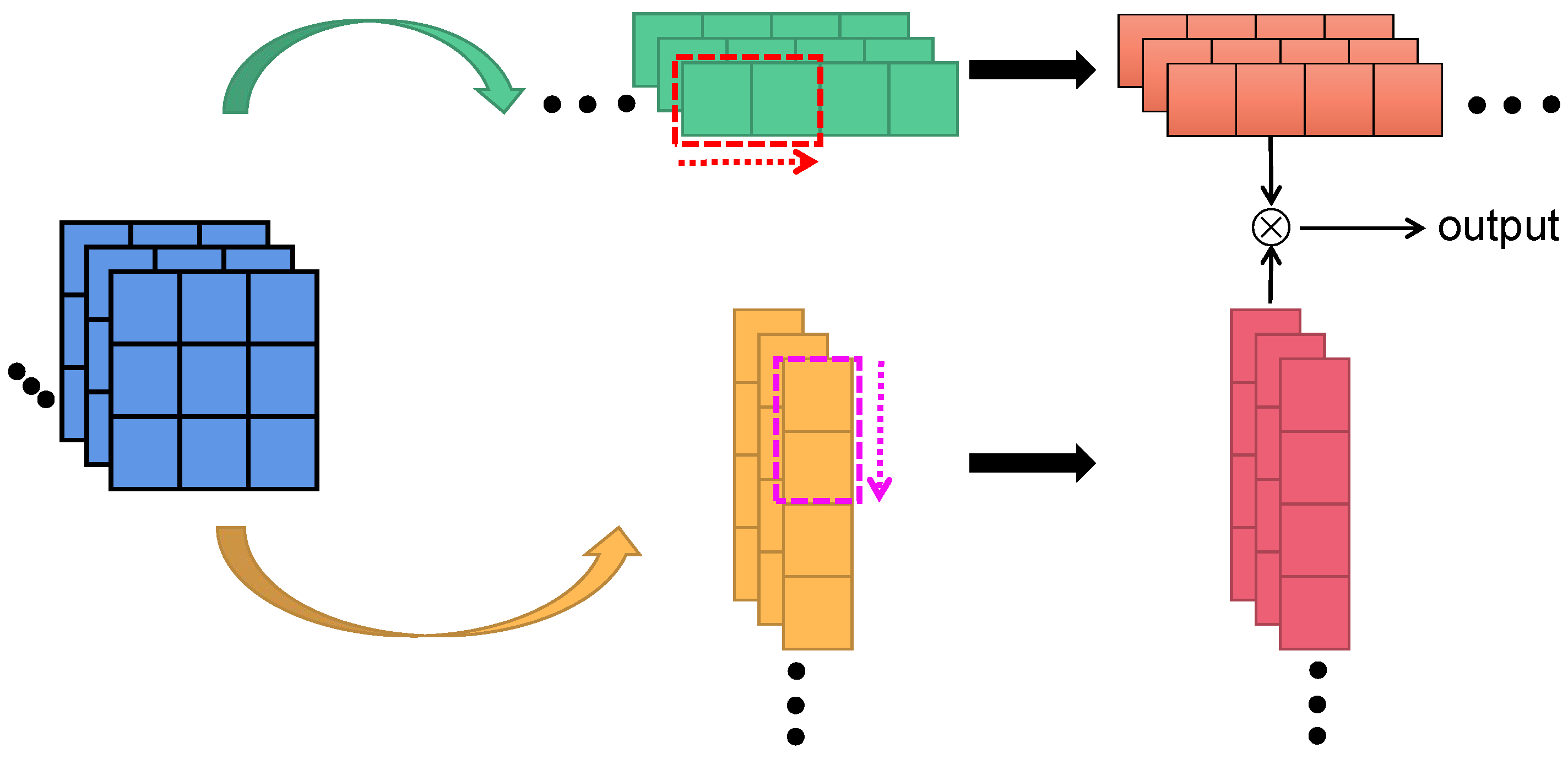
As shown in the Figure 7, after the dynamic motion capture, the spatio-temporal feature $X_i$ obtained by us is transformed into two different dimensional features $(N\ast T,C,H)$ and $(N\ast H,C,T)$. On this basis, in order to gather and merge the temporal information more closely, we take the operation in the following expression:

$$SpatialFunction=maxpool+avgpool$$

(13)

In the spatial dimension, two different pooling strategies are used by us to obtain salient spatial features.

In order to obtain more distinguishing spatio-temporal feature, we have adopted two different scales for utilizing spatial functions (that is, two different convolution kernels, 5 and 3, respectively). Then, in order to make the spatial and temporal features have better feature expression ability at the corresponding feature points, we use two 1D convolutions in the temporal dimension to obtain prominent temporal information ($TF$):

$$TemporalFunction=Sigmoid\left(conv1d\right(bn\left(conv1d\right(\left)\right)\left)\right)$$

(14)

Then, in order to balance the spatio-temporal features and highlight the key discriminative feature vectors, we performed the following operations on the spatio-temporal information (SF denotes SpatialFunction, TF represents TemporalFunction):

$$output=SF\left(x\right)\ast TF\left(x\right)+TF\left(x\right)\ast x$$

(15)

3.5. Interval Module Design

3.5.1. Learning Ability to Preserve Spatial Feature

For the Interval-Frame sampling module we proposed, a naive idea is to apply it at the beginning of the network, but due to the important role of spatial features in gait representation, we need to maintain the learning ability of spatial features, so that the final representation is rich in spatial information. Therefore, there are requirements for the application position of the Interval-Frame module. We believe that replacing the input of the network structure with Interval-Frame will destroy the integrity of the spatial frame-level features and reduce the learning ability of spatial features. It is a good choice to apply after frame-level feature extraction, which can get more information about subtle changes in body parts or joints (The final experimental results in Section 4.4.3 also validate our ideas).

3.5.2. Increase the Learning Ability of Temporal Information

After solving the problem of where to apply, a natural question is how to implement this sampling method. Inspired by [29], we designed two combinations strategies: one is to directly replace the original input as an interval frame (as shown in Figure 8a), and the other is to use a residual structure (as shown in Figure 8b); we believe that because the interval frame is incomplete in the temporal dimension, if the original frame sequence is directly replaced by the interval frame sequence, it will destroy the learning ability of temporal information and destroy the richness of features in the temporal dimension. We verified this in our ablation experiments, below in Section 4.4.4.

4. Results

4.1. DataSets

At present, the commonly used datasets in the field of gait recognition are CASIA-B [30] and OU-MVLP [31]. CASIA-B [30] is a smaller dataset in the field of gait recognition. It is often used to evaluate the effectiveness of the algorithm. There are 124 subjects’ multi-view gait contour data. Each subject in CASIA-B [30] is collected from 11 perspectives. The shooting angle starts from $0^{\circ }$, increases by ${18}^{\circ }$ each time, and ends at ${180}^{\circ }$. There are 10 sequences under each shooting angle, which are collected from three different conditions. That is, under normal walking conditions (NM: #01–06), walking with a bag carrying (#01–02), and walking with wearing a coat (#01–02), CASIA-B [30] has 124 × 11 × 10 gait sequences in total. OU-MVLP [31] is a large-scale common gait dataset; It is often used to verify the generalization capacity of the algorithm. Compared with CASIA-B [30], OU-MVLP [31] contains more subjects. It collected gait data from 10,307 subjects. Each subject was collected from 14 different angles, starting from $0^{\circ }$, increasing ${15}^{\circ }$ each time to ${270}^{\circ }$. Each angle contain two sequences (#01–02).

4.2. Implementation Details

4.2.1. Dataset Partition Criteria

Since neither of these two gait datasets include official training and test subset partitions, we use the same dataset division standard as [17]. For CASIA-B [30], it is divided into Large-Sample Training (LT), Medium-Sample Training (MT), and Small-Sample Training (ST) according to the size of the training sets. LT/MT/ST, respectively, use the first 74/62/24 subjects as the training sets, and the remaining 50/62/100 subjects as the test sets. For the test set of the above three settings, the 10 sequences contained in each subject are divided into gallery and three probe subsets, i.e., gallery: NM#01–04, probe: NM#05–06, BG#01–02, CL#01–02. For OUMVLP [31], the first 5153 subjects are used as training sets, and the last 5154 subjects are used as test sets. In the test phase, #01 is used as the gallery and #00 as the probe.

4.2.2. Parameter Settings

All our experiments were carried out on a computer containing 4 NVIDIA 3090. The same alignment method as [31] is used for each frame, and each frame is resized to the size of 64 × 44. The Adam [32] optimizer is the optimization method we used to train our model. The learning rate is set to 1 $\times {10}^{-4}$ and momentum is set to 0.2. We use the same sampling method as [23] to obtain our input sequence. During the process of training, the loss function we used is batch all+ separate triplet loss [33], the margin of which was set to 0.2. The format of batch size used in this experiment is (P, K), where P refers to the number of objects to be identified, and K refers to the number of sample sequences contained in each object. Specifically, in the experiment of CASIA-B [30], this paper sets batch size to (8,12), the number of iterations of training is 120 k. Due to the increase in the number of objects in OU-MVLP [31] samples, we change batch size to (32,10), the number of iterations of training is 250 k.

4.3. Compared with State-of-the-Art Methods

4.3.1. CASIA-B

As shown in

Table 1. Average rank-1 accuracy (%) on CASIA-B dataset under three different experimental settings, excluding identical-view cases.

Gallery NM #1–4			$0^{\circ }$–${180}^{\circ }$											Mean
	Probe		$0^{\circ }$	${18}^{\circ }$	${36}^{\circ }$	${54}^{\circ }$	${72}^{\circ }$	${90}^{\circ }$	${108}^{\circ }$	${126}^{\circ }$	${144}^{\circ }$	${162}^{\circ }$	${180}^{\circ }$
LT (74)	NM (#5–6)	GaitSet [4]	90.8	97.9	99.4	96.9	93.6	91.7	95.0	97.8	98.9	96.8	85.8	95.0
		GaitPart [7]	94.1	98.6	99.3	98.5	94.0	92.3	95.9	98.4	99.2	97.8	90.4	96.2
		GaitSlice [14]	95.5	99.2	99.6	99.0	94.4	92.5	95.0	98.1	99.7	98.3	92.9	96.7
		GaitGL [18]	96.0	98.3	99.0	97.9	96.9	95.4	97.0	98.9	99.3	98.8	94.0	97.5
		CSTL [22]	97.2	99.0	99.2	98.1	96.2	95.5	97.7	98.7	99.2	98.9	96.5	97.8
		Ours	96.9	99.3	99.3	98.8	97.8	96.2	97.9	99.2	99.6	99.4	96.4	98.3
	BG (#1–2)	GaitSet [17]	83.8	91.2	91.8	88.8	83.3	81.0	84.1	90.0	92.2	94.4	79.0	87.2
		GaitPart [23]	89.1	94.8	96.7	95.1	88.3	84.9	89.0	93.5	96.1	93.8	85.8	91.5
		GaitSlice [19]	90.2	96.4	96.1	94.9	89.3	85.0	90.9	94.5	96.3	95.0	88.1	92.4
		GaitGL [18]	92.6	96.6	96.8	95.5	93.5	89.3	92.2	96.5	98.2	96.9	91.5	94.5
		CSTL [22]	91.7	96.5	97.0	95.4	90.9	88.0	91.5	95.8	97.0	95.5	90.3	93.6
		Ours	94.0	97.6	98.4	97.2	93.3	92.0	94.0	97.1	98.2	97.1	92.9	95.6
	CL (#1–2)	GaitSet [17]	61.4	75.4	80.7	77.3	72.1	70.1	71.5	73.5	73.5	68.4	50.0	70.4
		GaitPart [23]	70.7	85.5	86.9	83.3	77.1	72.5	76.9	82.2	83.8	80.2	66.5	78.7
		GaitSlice [19]	75.6	87.0	88.9	86.5	80.5	77.5	79.1	84.0	84.8	83.6	70.1	81.6
		GaitGL [18]	76.6	90.0	90.3	87.1	84.5	79.0	84.1	87.0	87.3	84.4	69.5	83.6
		CSTL [22]	78.1	89.4	91.6	86.6	82.1	79.9	81.8	86.3	88.7	86.6	75.3	84.2
		Ours	83.7	93.4	95.5	91.7	86.9	84.5	88.1	91.5	92.5	90.4	79.0	88.8

, in order to verify the effectiveness of our proposed algorithm, we have listed the accuracy comparison results of the SOTA method and our algorithms. Among them, our method is 0.5%, 1.1%, 4.6% higher than the current best methods in the average recognition accuracy of Rank-1 in the LT settings under NM/BG/CL condition respectively. It is worth noting that our algorithm greatly improves the accuracy of BG and CL conditions. The gap between NM and BG reduce to within 3% (only 2.7%) when NM reaches above 98.0% of the recognition accuracy, and the gap between NM and CL reduce to within 10% (only 6.8%).

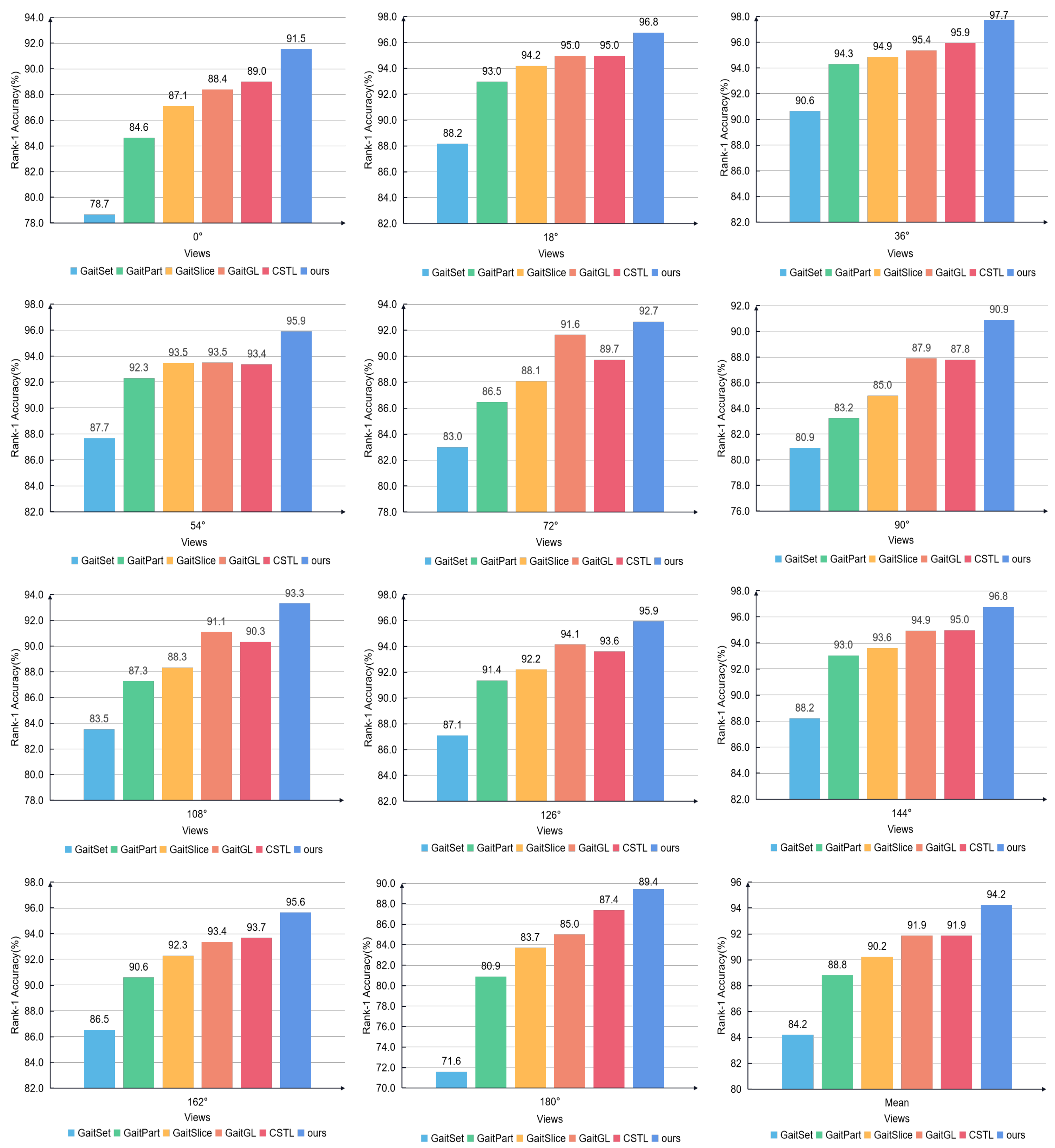
Figure 9 shows the comparison between our method and other state-of-the-art methods from 11 different viewpoints. As shown in the Figure 9, our method has higher recognition accuracy than other methods; when the viewing angle is ${90}^{\circ }$, the accuracy improvement is the largest (↑3.0%), and at ${72}^{\circ }$, the improvement is the smallest, also reaching 1.1%. Among them, the accuracy improvement at view of $0^{\circ },{54}^{\circ },{108}^{\circ },{126}^{\circ },{162}^{\circ },{180}^{\circ }$ all exceeded 2.0%. The average improvement accuracy of 11 viewing angles was 2.3%.

4.3.2. OU-MVLP

The experimental results under OU-MVLP prove that our algorithm has good generalization ability. As shown in the

Table 2. Average rank-1 accuracy on OU-MVLP across different views, excluding identical-view cases.

Probe	Gallery All 14 Views
	GaitSet [17]	GaitPart [23]	GaitSlice [19]	GaitGL [18]	CSTL [22]	Ours
$0^{\circ }$	79.5	82.6	84.1	84.9	87.1	87.3
${15}^{\circ }$	87.9	88.9	89	90.2	91.0	91.2
${30}^{\circ }$	89.9	90.8	91.2	91.1	91.5	91.5
${45}^{\circ }$	90.2	91.0	91.6	91.5	91.8	92.0
${60}^{\circ }$	88.1	89.7	90.6	91.1	90.6	91.1
${75}^{\circ }$	88.7	89.9	89.9	90.8	90.8	91.0
${90}^{\circ }$	87.8	89.5	89.8	90.3	90.6	90.9
${180}^{\circ }$	81.7	85.2	85.7	88.5	89.4	89.5
${195}^{\circ }$	86.7	88.1	89.3	88.6	90.2	90.5
${210}^{\circ }$	89.0	90.0	90.6	90.3	90.5	90.7
${225}^{\circ }$	89.3	90.1	90.7	90.4	90.7	91.0
${240}^{\circ }$	87.2	89.0	89.8	89.6	89.8	90.1
${255}^{\circ }$	87.8	89.1	89.6	89.5	90.0	90.1
${270}^{\circ }$	86.2	88.2	88.5	88.8	89.4	89.5
Mean	87.1	88.7	89.3	89.7	90.2	90.5

, the recognition accuracy of our algorithm under 14 different angles of view is more than that of the current SOTA method, of which the most obvious angle of improvement is ${60}^{\circ }$ (↑0.5%), the angle with the smallest accuracy improvement is ${30}^{\circ }$. The average recognition accuracy has reached 90.5% that is higher than the current optimal method.

4.4. Ablation Study

4.4.1. Effectiveness of Each Module

In order to explore the effectiveness of each module in our model, we conducted corresponding experiments, and the experimental results are shown in the

Table 3. Ablation study on the effectiveness of each module in our model.

Model		Rank-1 Accuracy (%)
		NM	BG	CL	Mean
GaitSet [17]		95.0	87.2	70.4	88.0
GaitPart [23]		96.2	91.5	78.7	88.0
GaitSlice [19]		96.7	92.4	81.6	88.0
GaitGL [18]		97.4	94.5	83.6	91.8
CSTL [22]		97.8	93.6	84.2	91.9
Ours	Baseline	97.2	92.6	82.4	90.7
	TSFE + Baseline	97.3	93.5	83.2	91.3
	Baseline + DMC	97.5	94.2	84.3	92.0
	Baseline + ODB	98.0	93.9	83.9	91.9
	Baseline + TSFE + DMC + ODB	98.3	95.6	88.8	94.2

. It is worth noting that our baseline uses four 2D convolutional layers as the frame-level feature extraction layer, and the micro-motion capturer in GaitPart as a temporal information pooling layer, together they form our baseline. As can be seen from the Table 3, each module we propose improves the recognition accuracy. Among them, after replacing TSFE with the frame-level feature extraction layer, the average recognition accuracy under the three conditions is improved 0.6%. After adding DMC, the recognition accuracy of the two complex conditions BG/CL is significantly improved 1.3%/1.5%, respectively. Replace MCM with After ODB, the recognition accuracy under NM has improved 0.8%.

4.4.2. Impact of the Dilation Operation in Temporal Dimension

In order to explore the impact of the dilated convolution on our proposed Temporal-Sensitive Feature Extractor, we conducted related experiments to explore this. Specifically, we explored the convolution used in the temporal feature dimension. First, we only used dilated convolution in the first layer, and then changed the first to fourth layers to use dilated convolution.

From the

Table 4. The impact of where and how Interval-Frame is used.

Where	How	Rank-1 Accuracy (%)
		NM	BG	CL	Mean
Before	In-Place	97.0	93.2	83.8	92.3
Before	Residual	97.3	94.0	84.0	92.8
After	In-Place	97.5	93.3	84.1	92.7
After	Residual	98.3	95.6	88.8	94.2

, we can see that the average recognition accuracy of only using dilated convolution in the first layer is 0.5% higher than that of not using dilated convolution, and then, using dilated convolution in the first two layers, the recognition accuracy under the three conditions (NM/BG/CL) were improved, and the average accuracy improved by 1.1% compared with the use of regular convolution. After that, using dilated convolution in the first three layers and first four layers, the accuracy of NM still increases, but in the BG condition, the accuracy began to fluctuate, and in CL condition, the accuracy even declined. The average rank-1 accuracy dropped by 0.1%. Therefore, we infer that since the dilated convolution has a larger receptive field under the same parameters settings, it will extract richer temporal features, but it is precisely because of this feature that aliasing information may be introduced in the feature extraction process, which also shows that, under normal walking conditions, the accuracy continues to increase with the increase in the number of dilated convolution layers, but under complex conditions (BG, CL), beyond a certain range, the recognition accuracy will fluctuate or even decline.

In order to more intuitively and clearly show the impact of the dilation operation of the temporal dimension on our model, we plotted the rank-1 accuracy under the above five setting conditions with the number of iterations in the Section 5, as shown in the Figure 10 and

Table 5. Rank-1 accuracy (%) under different dial settings (under CASIA-B, LT settings).

Settings	Rank-1 Accuracy (%)
	NM	BG	CL	Mean
no_dilation	97.6	94.9	88.1	93.5
dilation_in_first_layer	97.3	94.9	89.9	94.0
dilation_in_first_two_layers	97.6	95.5	90.6	94.6
dilation_in_first_three_layers	98.1	95.5	89.3	94.3
dilation_in_first_four_layers	98.3	95.6	88.8	94.2

.

4.4.3. Impact of Interval Frame Module

Regarding where to apply interval frame sampling and how to apply interval frame sampling, we conducted a series of related experiments to verify this. We sampled two strategies for where to apply interval frame sampling. In the network input (that is, before frame-level feature extraction) and after frame-level feature extraction, there are also two strategies for usage, which are the in-place and residual structures introduced in Section 3.4.2. The experimental results are shown in the following Table 4: after frame-level feature extraction, the residual structure achieved the best results, and replacing the residual with the in-place structure, the average recognition accuracy dropped by 1.5% under the three conditions. Replacing the usage position with the beginning of the network lost 1.4% of the average accuracy.

4.4.4. Impact of Interval Frame Sampling Distance

In order to explore the influence of the interval frame distance on the recognition accuracy, we set different interval frame distances (0, 1, 2, 3) and carried out corresponding comparative experiments. The experimental results are shown in the

Table 6. Influence of interval distance on experimental results.

The Gap of Interval Frame	Rank-1 Accuracy (%)
	NM	BG	CL	Mean
0	98.1	95.6	85.8	93.2
1	98.3	95.6	88.8	94.2
2	98.0	95.7	86.6	93.4
3	97.5	95.0	85.0	92.5

, from which we can see that when the interval frame is 1, the best effect can be obtained; compared with no interval frame, the average accuracy is increased by about 1.0%; increasing the interval frame distance to 2, BG and CL improves compared with the original frame sequence, but the accuracy of NM fluctuates. Continuing to increase the interval frame distance to 3, the accuracy decreased by 0.7%. We speculate that this is because the excessively long interval distance will alias with the original sequence, destroying the spatial structure of gait features, thereby reducing the learning ability of the network.

4.4.5. Impact of Different Concatenation Strategy

After using the interval frame strategy, depending on the distance d of the interval frame, we will obtain $d+1$ sub-sequences; after feature extraction of these sub-sequences, $d+1$ different feature matrices will be obtained. It is necessary to combine these feature matrices for feature mapping. In order to explore the optimal combination strategy, we conducted a series of experiments. The two naive ideas are addition and concatenation. When using the concatenation, in order to make the feature dimensions equal, we need to perform corresponding processing after concatenation. After the concatenation, the dimension of the feature will increase. Therefore, in order to keep the dimension of the feature unchanged, we have adopted three strategies and their combinations. These three strategies are AdaptiveAveragePool and AdaptiveMaxPool and a fully connected layers using 1D convolution.

It can be seen from the

Table 7. Rank-1 recognition accuracy under different feature combination strategies, where the concatenation operation is performed in the height dimension.

Addition	Concatenation			Rank-1 Accuracy (%)
	AdaptiveAvgPool	AdaptiveMaxPool	1D-Convolution	NM	BG	CL	Mean
✓	✕	✕	✕	98.0	95.3	89.0	94.1
✕	✓	✕	✕	98.3	95.6	88.8	94.2
✕	✕	✓	✕	97.8	95.2	88.5	93.8
✕	✕	✕	✓	97.2	94.5	85.2	92.3
✕	✓	✓	✕	98.1	95.3	88.5	94.0
✕	✓	✕	✓	97.0	93.2	84.1	91.4
✕	✕	✓	✓	97.1	93.8	85.0	92.0
✕	✓	✓	✓	97.3	94.2	84.2	91.9

that when adding the feature matrices obtained from different interval sub-sequences and the original frame sequence, these will complement each other, and recognition accuracy under CL exceeds 89.0%. After using the concatenation on channel dimension, the use of AdaptiveAveragePool balances the characteristics of each subsequences and achieves the best result. Using AdaptiveMaxPool reduces the average recognition accuracy by 0.4%. The use of only a fully connected layer to fix the output dimension is less effective, and the average recognition accuracy drops by 1.8% compared with the addition.

5. Discussion

The existing feature extraction backbone mainly uses a well-designed model to focus on feature extraction, such as [34,35,36,37,38,39,40], or weakly supervised/self-supervised methods for feature extraction, such as [41,42,43,44,45], or the use of some smart sensors for auxiliary feature extraction, such as [46,47,48,49]. Among them, using a unified model for feature extraction is currently the most commonly used method for vision-based gait recognition, and weakly supervised or even unsupervised learning is currently less used in the field of gait recognition, because it does not require data to be labeled. This indicates a new direction for future development due to the need to mine the internal relationship and characteristics of the data. Using unsupervised methods may cause the problem that the intra-class distance is larger than the inter-class distance; this is also one of the keys to feature extraction for gait recognition using unsupervised learning. The use of mobile phone sensors and other sensors for gait recognition can increase the gait information and improve the accuracy of gait information. Combining it with visual information and using multi-modal research can further increase the accuracy of gait recognition, which indicates another path for us in the future research.

In order to explore the advantages of the model and the existing related problems, we analyze the relevant indicators of the experiment (the experiment process was carried out under the CASIA-B data set and LT setting). Figure 11 shows how the loss varies with the number of iterations during training. This figure shows that the loss gradually decreases with the increase in the number of iterations, and finally tends to be stable when it is close to 120K, and the model converges. It shows that our model fits the data well.

The test results are also mutually verified with the above process, which proves the effectiveness of our model. As shown in Figure 10, in order to more intuitively and clearly show the impact of the dilation operation of the temporal dimension on our model, we plotted the rank-1 accuracy under the above five settings in Section 4.4.2 with the number of iterations; we can see that, in general, the recognition accuracy of our model under the three conditions increases continuously with the increase in the number of iterations, reaches a maximum value, and then begins to fluctuate near the optimal value. There are two exceptions, that is, under CL conditions, the first three layers are changed to use dilation convolution and the first four layers are changed to use dilation convolution. The recognition accuracy under CL conditions reaches the optimal value. After that, instead of fluctuating, it starts to decline, which shows that our model degrades under this condition, which is also consistent with our analysis in Section 4.4.2.

6. Conclusions

In this paper, we propose an interval frame sampling strategy and an Omni-Domain Feature Extraction Network for gait recognition that can enrich temporal information and improve the relevance of spatio-temporal information. The network consists of three main modules: (1) Temporal-Sensitive Feature Extractor; (2) Dynamic Motion Capture; (3) Omni-Domain Feature Balance Module. The first two modules can jointly strengthen the internal relationship between the characteristics of each gait frame. The last module further explore the fine-grained spatio-temporal features and make the obtained gait spatio-temporal features close to the internal relationship of gait as much as possible to improve the representation ability of the acquired features. Finally, we conducted many experiments, and the experimental results show that our method produces competitive results and good generalization ability.

References

1. Sarkar, S.; Liu, Z.; Subramanian, R. Gait recognition. In Encyclopedia of Cryptography, Security and Privacy; Springer: Berlin/Heidelberg, Germany, 2021; pp. 1–7. [Google Scholar]
2. Nixon, M. Model-based gait recognition. In Enclycopedia of Biometrics; Springer: Berlin/Heidelberg, Germany, 2009. [Google Scholar]
3. Liao, R.; Cao, C.; Garcia, E.B.; Yu, S.; Huang, Y. Pose-based temporal–spatial network (PTSN) for gait recognition with carrying and clothing variations. In Proceedings of the Biometric Recognition: 12th Chinese Conference, CCBR 2017, Shenzhen, China, 28–29 October 2017; Proceedings 12. Springer: Cham, Switzerland, 2017; pp. 474–483. [Google Scholar]
4. Liao, R.; Yu, S.; An, W.; Huang, Y. A model-based gait recognition method with body pose and human prior knowledge. Pattern Recognit. 2020, 98, 107069. [Google Scholar] [CrossRef]
5. Li, X.; Makihara, Y.; Xu, C.; Yagi, Y.; Yu, S.; Ren, M. End-to-end model-based gait recognition. In Proceedings of the Asian Conference on Computer Vision, Kyoto, Japan, 30 November–4 December 2020. [Google Scholar]
6. Teepe, T.; Khan, A.; Gilg, J.; Herzog, F.; Hörmann, S.; Rigoll, G. Gaitgraph: Graph convolutional network for skeleton-based gait recognition. In Proceedings of the 2021 IEEE International Conference on Image Processing (ICIP), Anchorage, AK, USA, 19–22 September 2021; pp. 2314–2318. [Google Scholar]
7. Liu, X.; You, Z.; He, Y.; Bi, S.; Wang, J. Symmetry-Driven hyper feature GCN for skeleton-based gait recognition. Pattern Recognit. 2022, 125, 108520. [Google Scholar] [CrossRef]
8. Yin, Z.; Jiang, Y.; Zheng, J.; Yu, H. STJA-GCN: A Multi-Branch Spatial–Temporal Joint Attention Graph Convolutional Network for Abnormal Gait Recognition. Appl. Sci. 2023, 13, 4205. [Google Scholar] [CrossRef]
9. Fu, Y.; Meng, S.; Hou, S.; Hu, X.; Huang, Y. GPGait: Generalized Pose-based Gait Recognition. arXiv 2023, arXiv:2303.05234. [Google Scholar]
10. Liao, R.; Li, Z.; Bhattacharyya, S.S.; York, G. PoseMapGait: A model-based gait recognition method with pose estimation maps and graph convolutional networks. Neurocomputing 2022, 501, 514–528. [Google Scholar] [CrossRef]
11. Cao, Z.; Simon, T.; Wei, S.E.; Sheikh, Y. Realtime multi-person 2d pose estimation using part affinity fields. In Proceedings of the IEEE Conference on Computer Vision and Pattern Recognition, Honolulu, HI, USA, 21–26 July 2017; pp. 7291–7299. [Google Scholar]
12. Sun, K.; Xiao, B.; Liu, D.; Wang, J. Deep high-resolution representation learning for human pose estimation. In Proceedings of the IEEE/CVF Conference on Computer Vision and Pattern Recognition, Long Beach, CA, USA, 16–20 June 2019; pp. 5693–5703. [Google Scholar]
13. Lin, T.Y.; Maire, M.; Belongie, S.; Hays, J.; Perona, P.; Ramanan, D.; Dollár, P.; Zitnick, C.L. Microsoft coco: Common objects in context. In Proceedings of the Computer Vision—ECCV 2014: 13th European Conference, Zurich, Switzerland, 6–12 September 2014; Proceedings, Part V 13. Springer: Cham, Switzerland, 2014; pp. 740–755. [Google Scholar]
14. Cao, Z.; Hidalgo, G.; Simon, T.; Wei, S.E.; Sheikh, Y. OpenPose: Realtime Multi-Person 2D Pose Estimation Using Part Affinity Fields. IEEE Trans. Pattern Anal. Mach. Intell. 2021, 43, 172–186. [Google Scholar] [CrossRef] [Green Version]
15. Fang, H.S.; Li, J.; Tang, H.; Xu, C.; Zhu, H.; Xiu, Y.; Li, Y.L.; Lu, C. Alphapose: Whole-body regional multi-person pose estimation and tracking in real-time. IEEE Trans. Pattern Anal. Mach. Intell. 2022, 45, 7157–7173. [Google Scholar] [CrossRef]
16. Song, Y.F.; Zhang, Z.; Shan, C.; Wang, L. Stronger, faster and more explainable: A graph convolutional baseline for skeleton-based action recognition. In Proceedings of the 28th ACM International Conference on Multimedia, Seattle, WA, USA, 12–16 October 2020; pp. 1625–1633. [Google Scholar]
17. Chao, H.; He, Y.; Zhang, J.; Feng, J. Gaitset: Regarding gait as a set for cross-view gait recognition. In Proceedings of the AAAI Conference on Artificial Intelligence, Honolulu, HI, USA, 27 January–1 February 2019; Volume 33, pp. 8126–8133. [Google Scholar]
18. Lin, B.; Zhang, S.; Yu, X. Gait recognition via effective global-local feature representation and local temporal aggregation. In Proceedings of the IEEE/CVF International Conference on Computer Vision, Montreal, BC, Canada, 11–17 October 2021; pp. 14648–14656. [Google Scholar]
19. Li, H.; Qiu, Y.; Zhao, H.; Zhan, J.; Chen, R.; Wei, T.; Huang, Z. GaitSlice: A gait recognition model based on spatio-temporal slice features. Pattern Recognit. 2022, 124, 108453. [Google Scholar] [CrossRef]
20. Hou, S.; Cao, C.; Liu, X.; Huang, Y. Gait lateral network: Learning discriminative and compact representations for gait recognition. In Proceedings of the Computer Vision–ECCV 2020: 16th European Conference, Glasgow, UK, 23–28 August 2020; Proceedings, Part IX. Springer: Cham, Switzerland, 2020; pp. 382–398. [Google Scholar]
21. Qin, H.; Chen, Z.; Guo, Q.; Wu, Q.J.; Lu, M. RPNet: Gait recognition with relationships between each body-parts. IEEE Trans. Circuits Syst. Video Technol. 2021, 32, 2990–3000. [Google Scholar] [CrossRef]
22. Huang, X.; Zhu, D.; Wang, H.; Wang, X.; Yang, B.; He, B.; Liu, W.; Feng, B. Context-sensitive temporal feature learning for gait recognition. In Proceedings of the IEEE/CVF International Conference on Computer Vision, Montreal, BC, Canada, 11–17 October 2021; pp. 12909–12918. [Google Scholar]
23. Fan, C.; Peng, Y.; Cao, C.; Liu, X.; Hou, S.; Chi, J.; Huang, Y.; Li, Q.; He, Z. Gaitpart: Temporal part-based model for gait recognition. In Proceedings of the IEEE/CVF Conference on Computer Vision and Pattern Recognition, Seattle, WA, USA, 14–19 June 2020; pp. 14225–14233. [Google Scholar]
24. Huang, Z.; Xue, D.; Shen, X.; Tian, X.; Li, H.; Huang, J.; Hua, X.S. 3D local convolutional neural networks for gait recognition. In Proceedings of the IEEE/CVF International Conference on Computer Vision, Montreal, BC, Canada, 11–17 October 2021; pp. 14920–14929. [Google Scholar]
25. Mogan, J.N.; Lee, C.P.; Lim, K.M.; Ali, M.; Alqahtani, A. Gait-CNN-ViT: Multi-Model Gait Recognition with Convolutional Neural Networks and Vision Transformer. Sensors 2023, 23, 3809. [Google Scholar] [CrossRef] [PubMed]
26. Yang, Y.; Yun, L.; Li, R.; Cheng, F.; Wang, K. Multi-View Gait Recognition Based on a Siamese Vision Transformer. Appl. Sci. 2023, 13, 2273. [Google Scholar] [CrossRef]
27. Chen, J.; Wang, Z.; Zheng, C.; Zeng, K.; Zou, Q.; Cui, L. GaitAMR: Cross-view gait recognition via aggregated multi-feature representation. Inf. Sci. 2023, 636, 118920. [Google Scholar] [CrossRef]
28. Sun, G.; Zhang, X.; Jia, X.; Ren, J.; Zhang, A.; Yao, Y.; Zhao, H. Deep fusion of localized spectral features and multi-scale spatial features for effective classification of hyperspectral images. Int. J. Appl. Earth Obs. Geoinf. 2020, 91, 102157. [Google Scholar] [CrossRef]
29. Lin, J.; Gan, C.; Han, S. Tsm: Temporal shift module for efficient video understanding. In Proceedings of the IEEE/CVF International Conference on Computer Vision, Seoul, Republic of Korea, 27–28 October 2019; pp. 7083–7093. [Google Scholar]
30. Yu, S.; Tan, D.; Tan, T. A Framework for Evaluating the Effect of View Angle, Clothing and Carrying Condition on Gait Recognition. In Proceedings of the 18th International Conference on Pattern Recognition (ICPR’06), Hong Kong, China, 20–24 August 2006; Volume 4, pp. 441–444. [Google Scholar] [CrossRef]
31. Takemura, N.; Makihara, Y.; Muramatsu, D.; Echigo, T.; Yagi, Y. Multi-view large population gait dataset and its performance evaluation for cross-view gait recognition. IPSJ Trans. Comput. Vis. Appl. 2018, 10, 1–14. [Google Scholar] [CrossRef] [Green Version]
32. Kingma, D.P.; Ba, J. Adam: A Method for Stochastic Optimization. arXiv 2017, arXiv:1412.6980. [Google Scholar]
33. Hermans, A.; Beyer, L.; Leibe, B. In Defense of the Triplet Loss for Person Re-Identification. arXiv 2017, arXiv:1703.07737. [Google Scholar]
34. Yu, S.; Chen, H.; Wang, Q.; Shen, L.; Huang, Y. Invariant feature extraction for gait recognition using only one uniform model. Neurocomputing 2017, 239, 81–93. [Google Scholar] [CrossRef]
35. Zhao, H.; Fang, Z.; Ren, J.; MacLellan, C.; Xia, Y.; Li, S.; Sun, M.; Ren, K. SC2Net: A Novel Segmentation-Based Classification Network for Detection of COVID-19 in Chest X-Ray Images. IEEE J. Biomed. Health Inform. 2022, 26, 4032–4043. [Google Scholar] [CrossRef]
36. Ma, P.; Ren, J.; Sun, G.; Zhao, H.; Jia, X.; Yan, Y.; Zabalza, J. Multiscale Superpixelwise Prophet Model for Noise-Robust Feature Extraction in Hyperspectral Images. IEEE Trans. Geosci. Remote Sens. 2023, 61, 1–12. [Google Scholar] [CrossRef]
37. Yan, Y.; Ren, J.; Zhao, H.; Windmill, J.F.; Ijomah, W.; De Wit, J.; Von Freeden, J. Non-destructive testing of composite fiber materials with hyperspectral imaging—Evaluative studies in the EU H2020 FibreEUse project. IEEE Trans. Instrum. Meas. 2022, 71, 1–13. [Google Scholar] [CrossRef]
38. Xie, G.; Ren, J.; Marshall, S.; Zhao, H.; Li, R.; Chen, R. Self-attention enhanced deep residual network for spatial image steganalysis. Digit. Signal Process. 2023, 139, 104063. [Google Scholar] [CrossRef]
39. Ren, J.; Sun, H.; Zhao, H.; Gao, H.; Maclellan, C.; Zhao, S.; Luo, X. Effective extraction of ventricles and myocardium objects from cardiac magnetic resonance images with a multi-task learning U-Net. Pattern Recognit. Lett. 2022, 155, 165–170. [Google Scholar] [CrossRef]
40. Fan, D.P.; Zhou, T.; Ji, G.P.; Zhou, Y.; Chen, G.; Fu, H.; Shen, J.; Shao, L. Inf-net: Automatic covid-19 lung infection segmentation from ct images. IEEE Trans. Med. Imaging 2020, 39, 2626–2637. [Google Scholar] [CrossRef] [PubMed]
41. Liu, D.; Cui, Y.; Yan, L.; Mousas, C.; Yang, B.; Chen, Y. Densernet: Weakly supervised visual localization using multi-scale feature aggregation. In Proceedings of the AAAI Conference on Artificial Intelligence, Virtually, 2–9 February 2021; Volume 35, pp. 6101–6109. [Google Scholar]
42. Li, Y.; Ren, J.; Yan, Y.; Liu, Q.; Ma, P.; Petrovski, A.; Sun, H. CBANet: An End-to-end Cross Band 2-D Attention Network for Hyperspectral Change Detection in Remote Sensing. IEEE Trans. Geosci. Remote Sens. 2023. [Google Scholar] [CrossRef]
43. Sun, G.; Fu, H.; Ren, J.; Zhang, A.; Zabalza, J.; Jia, X.; Zhao, H. SpaSSA: Superpixelwise Adaptive SSA for Unsupervised Spatial–Spectral Feature Extraction in Hyperspectral Image. IEEE Trans. Cybern. 2022, 52, 6158–6169. [Google Scholar] [CrossRef] [PubMed]
44. Sun, H.; Ren, J.; Zhao, H.; Yuen, P.; Tschannerl, J. Novel Gumbel-Softmax Trick Enabled Concrete Autoencoder With Entropy Constraints for Unsupervised Hyperspectral Band Selection. IEEE Trans. Geosci. Remote Sens. 2022, 60, 1–13. [Google Scholar] [CrossRef]
45. Fu, H.; Sun, G.; Zhang, A.; Shao, B.; Ren, J.; Jia, X. Unsupervised 3D tensor subspace decomposition network for hyperspectral and multispectral image spatial-temporal-spectral fusion. IEEE Trans. Geosci. Remote Sens. 2023, in press. [Google Scholar] [CrossRef]
46. Das, S.; Meher, S.; Sahoo, U.K. A Unified Local–Global Feature Extraction Network for Human Gait Recognition Using Smartphone Sensors. Sensors 2022, 22, 3968. [Google Scholar] [CrossRef] [PubMed]
47. Yan, Y.; Ren, J.; Tschannerl, J.; Zhao, H.; Harrison, B.; Jack, F. Nondestructive phenolic compounds measurement and origin discrimination of peated barley malt using near-infrared hyperspectral imagery and machine learning. IEEE Trans. Instrum. Meas. 2021, 70, 1–15. [Google Scholar] [CrossRef]
48. Chen, R.; Huang, H.; Yu, Y.; Ren, J.; Wang, P.; Zhao, H.; Lu, X. Rapid Detection of Multi-QR Codes Based on Multistage Stepwise Discrimination and A Compressed MobileNet. IEEE Internet Things J. 2023. [Google Scholar] [CrossRef]
49. Sergiyenko, O.Y.; Tyrsa, V.V. 3D optical machine vision sensors with intelligent data management for robotic swarm navigation improvement. IEEE Sens. J. 2020, 21, 11262–11274. [Google Scholar] [CrossRef]
Figure 1. Schematic diagram of interval frame sampling strategy. The interval frame sampling strategy is to complete the acquisition of interval frames based on the original frame at intervals of n frames. As shown in the figure, the middle gait sequence is the original frame sequence, and the upper two gait sequences are intervals of 1 frame (n = 1); below is the three interval frame gait sequence obtained when the interval is two frames (n = 2).
Mathematics 11 02612 g001
Figure 2. The overall structure of our proposed method. TSFE denotes Temporal-Sensitive Feature Extractor. DMC represents Dynamic Motion Capture. ODB represents Omni-Domain Feature Balance Module. FC denotes the Fully Connected Layer. TSFE captures the spatio-temporal patterns contained in raw sequences, and maps raw gait contours into low-level feature representations. After horizontal pooling and interval sampling, redundant spatial information is reduced and temporal information is enriched (yellow and green represent different feature maps, in order to indicate interval frame sampling). Afterwards, features with multi-scale temporal information are obtained through DMC. Finally, the temporal information and spatial information are balanced through ODB. Then, through the Fully Connected Layer, the final representation is obtained.
Mathematics 11 02612 g002
Figure 3. Operation Details of Temrpoal-Sensitive Feature Extractor. Colored rectangles represent feature maps, and dotted boxes represent convolution kernels; the orange diamond represents the specific operation, and its formula is shown in Equation (9). This operation consists of two parallel modules: the upper one is the 1D convolution operation in the temporal dimension, the lower one is the 2D convolution operation in the spatial dimension, ω is the parameters obtained in the 1D convolution, and λ is the parameters obtained by 2D convolution, the two sets of parameters and features are multiplied by input x and added to obtain the final low-level feature.
Mathematics 11 02612 g003
Figure 4. Schematic diagram of dilated convolution operation, (a) shows 2D dilated convolution, (b) shows 1D dilated convolution. The blue box is the receptive field corresponding to the convolution kernel. Dilated convolution has a larger receptive field than ordinary convolution, and more spatio-temporal information can be obtained by sliding the convolution kernel.
Mathematics 11 02612 g004
Figure 5. The schematic diagram of Dynamic Motion Capture (DMC). The blue rectangle represents feature vectors. 1D convolutions of different sizes have kernels of different sizes. It slides on the H * T dimension, and aggregates each adjacent 2r + 1 column vector in the multi-motion feature vector. (It is worth mentioning that convolution kernels of different sizes have different receptive fields. Therefore, the r corresponding to convolution kernels of different sizes is also different. For the convenience of description, we draw them together.) Four sets of different parameters ( α , β , γ , σ ) are obtained through the convolution of four different scales. Different parameters and features are operated to obtain multi-scale features; then, the final multi-scale spatio-temporal features are obtained through concatenation.
Mathematics 11 02612 g005
Figure 6. Details of weight distribution for multi-scale features.
Mathematics 11 02612 g006
Figure 7. Illustration of Omni-Domain Feature Balance Module. Colored rectangles represent feature maps, and dotted boxes represent convolution kernels. ODB contains two parallel modules, the upper branch is the 1D convolution operation of the temporal dimension, and the lower branch is the pooling kernel of the spatial dimension. Through the movement of different convolution kernels, salient temporal features and representative spatial features are obtained, respectively. Multiplying gives balanced salient spatio-temporal features.
Mathematics 11 02612 g007
Figure 8. The two application methods of interval frames we adopt, the left side (a) is the In-Place structure, which converts the original sequence into multiple interval frame sequences as input; the right side (b) is the residual structure, keeping the original sequence unchanged, fuse the original frame information and recombined interval frame information.
Mathematics 11 02612 g008
Figure 9. Under 11 different perspectives, the comparison of our method and other state-of-the-art methods, the average recognition accuracy under three different walking conditions (NM/BG/CL), in CASIA-B, LT settings.
Mathematics 11 02612 g009
Figure 10. Rank-1 accuracy (%) changes with the number of iterations under different dilation settings in temporal dimension (under three walking conditions (NM/BG/CL), CASIA-B, LT seetings).
Mathematics 11 02612 g010
Figure 11. Loss (a) and loss-num (b) change with the number of iterations (Under CASIA-B, LT settings).
Mathematics 11 02612 g011