1. Introduction
Since the 1990s, with the rapid development of information technology, the application of database systems has become more widespread, and at the same time database technology has entered a completely new stage, from solely managing some simple data to managing a wide variety of complex data such as images, videos, audio, graphics, and electronic files generated by various devices; therefore, the amount of data to process has become larger and larger [
1].
In this era of such advanced information, the vast amount of information does not only bring us benefits but also us many negative effects. The most important factor in the influence on negative effects is that effective information is hard to refine, and too much meaningless data will inevitably cause issues in terms of the loss of meaningful knowledge. This is what John Nalsbert calls the “information-rich but knowledge-poor” dilemma [
2]. With the original functions of database systems, people could not discover the relationships and rules implied in data, and could not predict future trends based on existing data. There is a lack of methods to uncover the hidden value behind data. To solve this problem, there is an urgent need for a technology that can analyze large amounts of information more deeply, obtain insight into its hidden value, and make seemingly useless data useful [
3].
Decision trees are an effective way to generate classifiers from data, and represent the class of the most widely applied logical methods for this purpose [
4,
5]. In 1980, Kass first proposed the chi-squared automatic interaction detector (CHAID), which is a tool used to discover relationships between variables, a decision tree technique based on an adjusted significance test (Bonferroni test) [
6,
7]. It divides the respondents into several groups according to the relationship between the underlying variable and the dependent variable, and then each group into several groups. Dependent variables are usually some key indicators, such as the level of use, purchase intention, etc. A dendrogram is displayed after each program run. The top is a collection of all respondents, the following is a subset of two or more branches, and the CHAID classification is based on a dependent variable [
8]. Classification and regression tree (CART) is a decision tree algorithm based on the binary tree structure of the Gini coefficient that supports regression and classification. It adopts the method of pruning, which is mainly used in the classification prediction of small- and medium-sized data [
9,
10]. Iterative Dichotomiser (ID3) is a decision tree algorithm based on information entropy that can only deal with categorical variables and is easily overfit, which mainly uses classification prediction on small data sets [
10,
11].
In practice, CHAID is often used in the context of direct selling, selecting consumer groups and predicting their responses, and determining how some variables affect other variables [
12,
13], while other early applications are in the research fields of medicine and psychiatry [
14,
15], as well as engineering project cost control, financial risk warning, and fire reception and handling analysis [
16,
17]. We are been starkly aware of the non-linear relationships among CHAID maps, and they can empower predictive models with stability [
18]. However, we do not precisely know how high its accuracy is. To find out the perfect scope the CHAID algorithm fits into, this paper presented an analysis of the accuracy of the CHAID algorithm. of the analysis was based on the introduction of the CHAID algorithm in the second part to obtain insight into the causes of the accuracy of the CHAID algorithm and the difference between several other commonly used decision tree algorithms [
19,
20]. In the third part, we used IBM SPSS Statistics 26.0 software and the Python 3.7 language to realize the differences between multiple decision trees while further comparing the differences between the three on the big data set of bike-sharing requirements.
3. Comparison of Decision Tree Algorithm and Accuracy Analysis of the CHAID Algorithm
The three most commonly used decision tree algorithms are CHAID, CART, and ID3, including the latest C4.5 and even C5.0.
The CHAID algorithm has a long history. According to the principle of local optimization, CHAID uses the chi-square test to select the independent variables that affect the dependent variable the most. Then, because the independent variables may have many different categories, the CHAID algorithm will generate equal amounts of leaf nodes according to the number of categories of the independent variable, so the CHAID algorithm is a multi-fork tree.
The CHAID method is optimal when the predictor variable is a categorical variable. For continuous variables, CHAID automatically divides the continuous variables into 10 segments, but there may be omissions.
The CHAID algorithm uses the chi-square detection method in statistics, and because of the chi-square detection method, CHAID has a good mathematical theoretical basis in branch calculation, and its credibility and its accuracy are relatively high.
On this basis, the CHAID algorithm uses the pre-pruning method; pre-pruning is pruning before dividing and generating the decision tree under constant pruning, so pre-pruning not only reduces the training time overhead and testing time overhead of the CHAID decision tree but also reduces the risk of overfitting. On the other hand, some pre-pruning divisions may not improve the generalization performance, or may even cause a temporary decrease in generalization performance, but subsequent divisions based on this division may lead to a significant improvement in generalization performance, thus posing the risk of underfitting. Therefore, if the number of pruning is maintained in a good interval when the amount of data is sufficient and the types are mostly categorical variables, the risk of underfitting of the CHAID algorithm will be further reduced and the accuracy will be further improved.
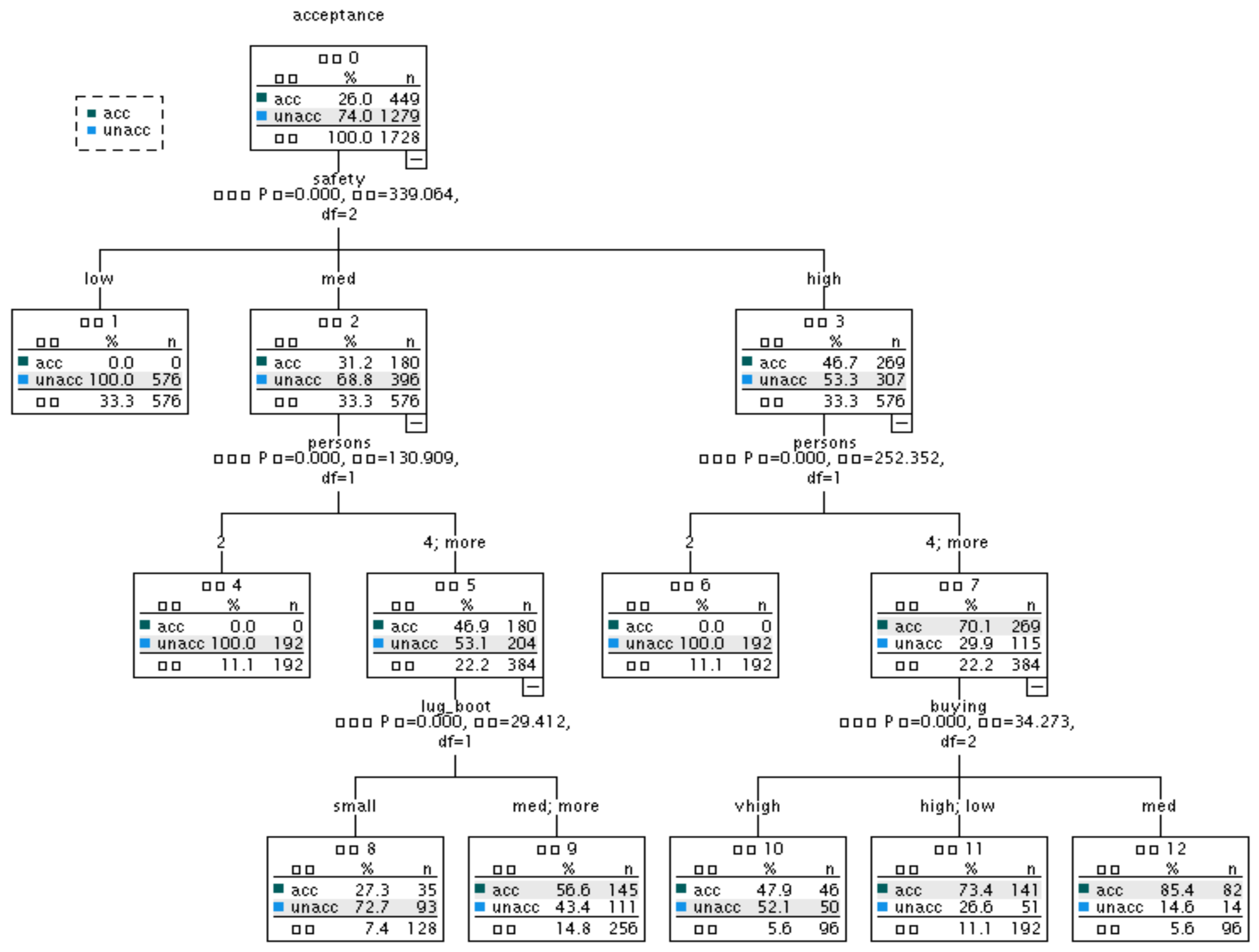
In
Figure 1, we can clearly see the significant correlation between features and car purchase intentions. In the first layer of the decision tree, we see that
= 339.064 of safety terms is the largest chi-square value and the most significant correlation among all feature terms. The remaining feature terms calculate the chi-square value again on the basis of the safety term, so we can clearly see the correlation degree of each feature, and this can also be used as a model to predict whether someone will buy a certain kind of car according to their characteristics.
As for the CART (Classification and Regression Tree) algorithm, its segmentation logic is the same as that for CHAID, and the division of each layer is based on the test and selection of all independent variables. However, the test standard used by CART is not the chi-square test, but the indicators of impurity, such as the Gini coefficient (Gini). The biggest difference between the two is that CHAID adopts the principle of local optimization, that is, the nodes are irrelevant to each other. After a node is determined, the following growth process is carried out completely within the node. CART, on the other hand, focuses on the overall optimization and adopts the post-pruning method, which makes the tree grow as much as possible, and then cuts the tree back and evaluates the non-leaf nodes in the tree from bottom to top, so the cost of training time is much larger than the pre-pruning decision tree.
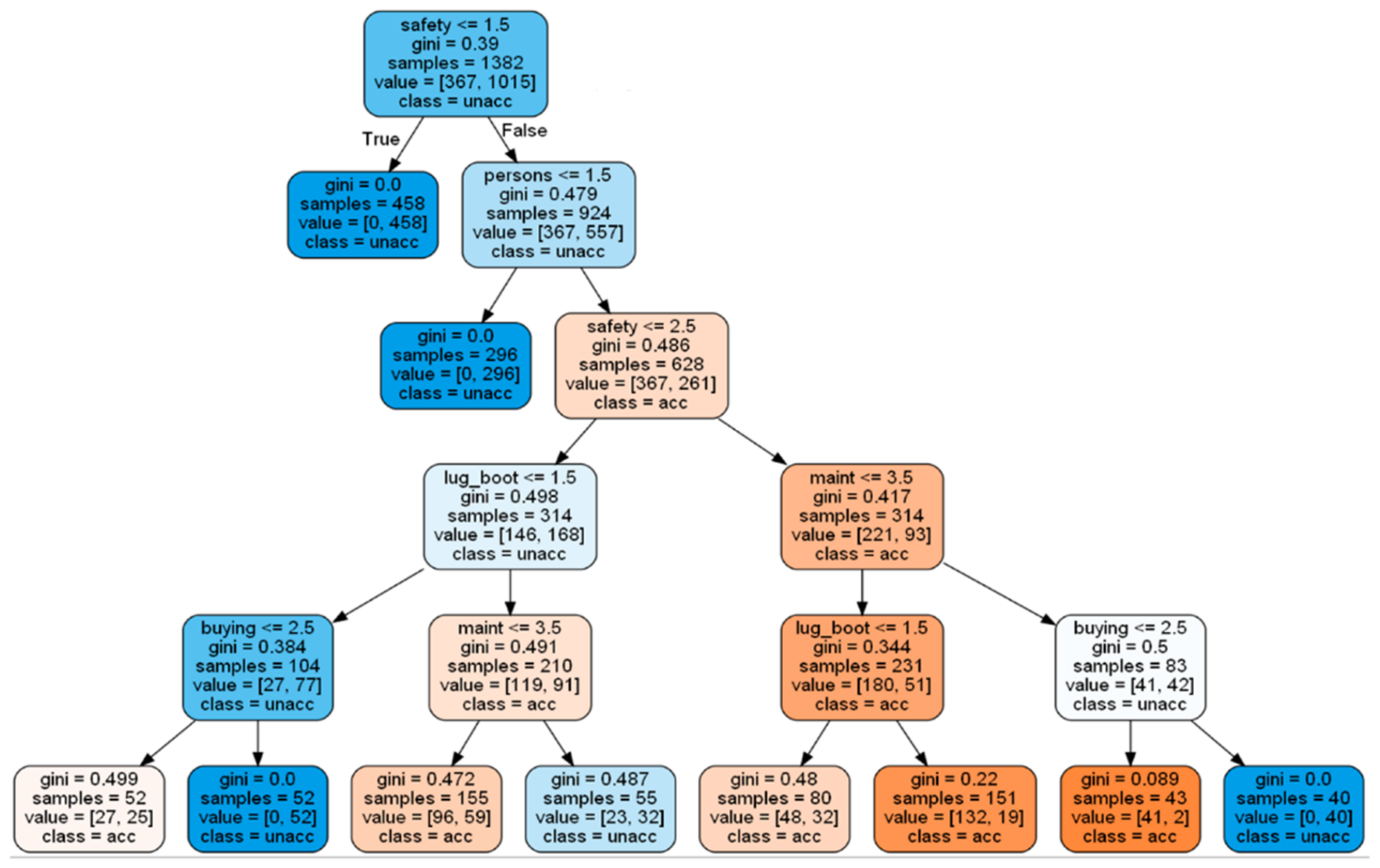
In
Figure 2, we can see that the gini = 0.39 of the safety term in the first layer of the decision tree is the smallest and the most relevant among all the feature terms. However, the feature term appears repeatedly, so it is impossible to intuitively see the importance of each feature, and it is more suitable for the model to predict whether someone will buy a certain kind of car according to their characteristics.
If there is missing data in the independent variable, CART can be used to find alternative data to replace the missing value, while CHAID takes the missing value as a separate type of value.
Among CART and CHAID, one is a binary tree and the other is a multi-fork tree; CART selects the best binary cut in each branch, so a variable is likely to be used multiple times in different trees; CHAID divides multiple statistically significant branches for one variable at a time, which will grow faster, but the support of the sub rapidly decreases compared with CART, approaching a bloated and unstable tree more quickly.
Therefore, after the number of data categories in the data set increases to a certain extent, the accuracy of the CHAID algorithm will have a large decrease compared with the CART algorithm. The number of features of the data can be reduced by removing some data irrelevant to the target data during the data cleaning so as to improve the accuracy of the CHAID algorithm.
The ID3 (Iterative Dichotomiser) algorithm and CART are in the same period; its biggest feature is that the independent variable selection criteria are based on the measure of information gain: the attribute with the highest information gain is selected as the split attribute of the node, and the result is the minimum information required to classify the segmented node, which is also an idea of division purity. As for the later development of C4.5, which can be understood as the development version of ID3, the main difference between the two is that C4.5 uses the information gain rate instead of the information gain measure in ID3. The main reason for such a replacement is that the information gain measure has a disadvantage, that is, it tends to choose attributes with a large number of values. As an extreme example, for the division of Member_Id, each Id is a pure group, but such a division has no practical significance. The information gain rate adopted by C4.5 can overcome this disadvantage. It adds a piece of split information to normalize constraints on the information gain. Additionally, C5.0 is the latest version. Compared with C4.5, C5.0 uses less memory and builds a smaller rule set than C4.5, while also being more accurate.
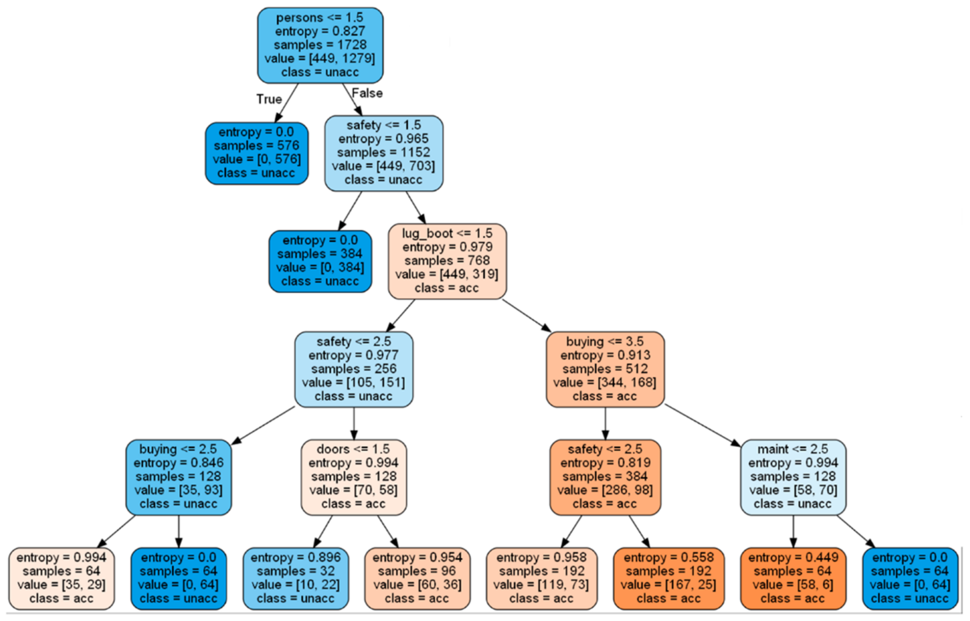
In
Figure 3, we can see that the features of the first layer of the decision tree term are persons, where persons entropy = 0.827 is the largest entropy among all, but the features will repeat, so can not intuitively see the importance of features; it is therefore more suitable for the model to make predictions according to the characteristics of an individual.
We also compared classification modeling using CHAID, CART, and ID3 decision tree algorithms on the large data set of bike-sharing requirements.
Table 7 clearly illustrates the distinctions among the three decision tree algorithms (CHAID, CART, and ID3), as well as the modeling and detection outcomes of these algorithms on large datasets of bike-sharing demand. The detection accuracy column shows that CHAID had a 92.3% accuracy on the shared bike data test set, indicating that it has excellent results in classification and prediction modeling on large data sets. CART, on the other hand, had an 85.7% accuracy, suggesting that its classification and prediction modeling on large data sets are not as good as CHAID and it is better suited for small and medium-sized data sets. ID3 had a 69.1% accuracy on the shared bike data test set, which indicates that its classification and prediction modeling on large data sets are prone to overfitting and it is better suited for small data sets.
4. Discussion
The decision tree algorithm belongs to the supervised learning machine learning method, and it is a commonly used technology in data mining. It can be used to classify the analyzed data, and it can also be used for prediction. Common algorithms are CHAID, CART, ID3, C4.5, C5.0, and so on. The second part is the study of the core idea of the CHAID decision tree algorithm and the classification process, the specific steps of the classification process, and the principle formula of the CHAID decision tree algorithm in the branching process. The third part is a comparison between the CHAID decision tree algorithm and other commonly used decision tree algorithms and a partial analysis of the accuracy of the CHAID algorithm. In this study, we provided an example of factor analysis for automobile satisfaction and implement an in-depth comparison using multiple decision tree algorithms. Additionally, we modeled and evaluated the accuracy of three decision tree algorithms—CHAID, CART, and ID3—on large datasets of bike-sharing demand. Through a thorough analysis of their accuracy, we examined the performance of these three decision tree algorithms on large datasets.
The CHAID algorithm uses chi-square detection and pre-pruning in the branch method, the CART is the Gini coefficient (Gini) pruning in the branch method. ID3 is a measure based on information gain, and C4.5 and C5.0 adopt information gain rate. CHAID and CART can process continuous data, while ID3 cannot; ID3 cannot process data with missing values, CHAID and CART can; with too many features in the data, CART and ID3 easily overfit, and CHAID is more stable than the previous two, and obtain more accurate results.
This paper leads us toward an in-depth understanding of these algorithms, letting us choose a relatively good decision tree algorithm for data mining according to our specific data. The application of the CHAID algorithm can also enable some countermeasures to address some factors affecting accuracy, so it is more conducive to obtaining a more accurate and better result.
Although there are some works have analyzed and compared CHAID, CART, and ID3, none of them based on the big data sets. We tested the CHAID, CART, and ID3 algorithms with a shared bike system which provides the big data set. This data set can enable a more in-depth understanding of the CHAID algorithm instead of the practical improvement on the CHAID algorithm.
In the next stage of research, we will find more data to compare these several decision tree algorithms, and further discuss the accuracy of the CHAID algorithm for use with different data. According to the experimental results, we can specifically summarize the differences between these decision tree algorithms and the influence of different data on the accuracy of the CHAID algorithm, as well as the differences between the accuracy of each algorithm. When we choose a decision tree algorithm according to the specific situation of the data, we can achieve a clearer and more intuitive understanding of the data and have a better understanding of the accuracy analysis of the CHAID algorithm.


