A New Entropy Stable Finite Difference Scheme for Hyperbolic Systems of Conservation Laws

Abstract

The hyperbolic problem has a unique entropy solution, which maintains the entropy inequality. As such, people hope that the numerical results should maintain the discrete entropy inequalities accordingly. In view of this, people tend to construct entropy stable (ES) schemes. However, traditional numerical schemes cannot directly maintain discrete entropy inequalities. To address this, we here construct an ES finite difference scheme for the nonlinear hyperbolic systems of conservation laws. The proposed scheme can not only maintain the discrete entropy inequality, but also enjoy high-order accuracy. Firstly, we construct the second-order accurate semi-discrete entropy conservative (EC) schemes and ensure that the schemes meet the entropy identity when an entropy pair is given. Then, the second-order EC schemes are used as a building block to achieve the high-order accurate semi-discrete EC schemes. Thirdly, we add a dissipation term to the above schemes to obtain the high-order ES schemes. The term is based on the Weighted Essentially Non-Oscillatory (WENO) reconstruction. Finally, we integrate the scheme using the third-order Runge–Kutta (RK) approach in time. In the end, plentiful one- and two-dimensional examples are implemented to validate the capability of the scheme. In summary, the current scheme has sharp discontinuity transitions and keeps the genuine high-order accuracy for smooth solutions. Compared to the standard WENO schemes, the current scheme can achieve higher resolution.

1. Introduction

In this article, we concentrate on constructing high-order numerical schemes. Because of the high nonlinearity of the governing equations, theoretical analysis is very difficult. Numerical solving by high-order schemes is an effective approach and has attracted extensive attention in the field of scientific computing [1,2,3]. The nonlinear systems in one-dimensional (1D) space read as

$${\mathbf{U}}_t+\mathbf{F}{\left(\mathbf{U}\right)}_x=0.$$

(1)

Representative research of high-order schemes for the nonlinear systems (1) mainly include: the kinetic scheme [4], gas-kinetic scheme [5], central-upwind scheme [6], weighted essentially non-oscillatory (WENO) schemes [7,8,9,10,11,12,13,14,15,16], Hermite WENO scheme [17], central schemes [18,19], the Runge–Kutta discontinuous Galerkin (RKDG) methods [20,21,22], ADER (Arbitrary DERivatives in space and time) schemes [23,24], spectral element method [25], Godunov-type method [26], element-free Galerkin method [27], and ADER-DG method [28]. For other high-order schemes, we refer to [29,30,31,32,33].

However, there may not be exact solutions when calculating the nonlinear systems of hyperbolic conservation laws (1). Therefore, we need to define the weak solutions in a distributional sense. However, these weak solutions may lack uniqueness. In fact, the entropy condition is significant in screening entropy solutions (physically relevant solutions) [34].

Definition 1

(Entropy function [35]). A strictly convex function $\eta \left(\mathbf{U}\right)$ can be an entropy function of the system (1), if there exists associated entropy fluxes $q\left(\mathbf{U}\right)$ such that

$$q^{\prime }\left(\mathbf{U}\right)={\mathbf{V}}^{\top }{\mathbf{F}}^{\prime }\left(\mathbf{U}\right),$$

(2)

where $\mathbf{V}={\eta }^{\prime }{\left(\mathbf{U}\right)}^{\top }$ is an entropy variable and $(\eta ,q)$ is known as an entropy pair.

With respect to the given entropy pair $(\eta ,q)$, multiplying both sides of (1) by ${\mathbf{V}}^{\top }$, the solutions which are smooth of (1) meet the following identity

$$\frac{\partial \eta \left(\mathbf{U}\right)}{\partial t}+\frac{\partial q\left(\mathbf{U}\right)}{\partial x}=0.$$

(3)

However, the above identity (3) no longer holds in the case of the emergence of discontinuous solutions. In particular, the entropy solution $\mathbf{U}$ meets the following inequality

$$\frac{\partial \eta \left(\mathbf{U}\right)}{\partial t}+\frac{\partial q\left(\mathbf{U}\right)}{\partial x}\le 0.$$

(4)

Generally, both the entropy identity (3) and the entropy inequality (4) are called as the entropy conditions. Theoretically, entropy conditions play a crucial role with respect to the well-posedness of the systems such as (1). Numerically, high-order schemes which meet the above inequality according to (4) can improve its own robustness. Therefore, it is significant to construct schemes meeting entropy inequality with regard to a given entropy pair. The schemes satisfying discrete entropy inequality are also called entropy stable (ES) schemes. In recent years, the research on ES schemes has attracted wide attention, such as in: the discontinuous Galerkin (DG) spectral element method [36] nodal DG method [37], DG methods [38,39], and finite difference schemes [40].

The main aim of this article is to present a high-order ES scheme for the systems. Firstly, we establish a two-point EC flux to construct a second-order EC scheme, which satisfies the entropy identity. Next, we achieve a high-order EC scheme based on the above scheme. However, there might be numerical oscillations around discontinuity. To overcome this shortcoming, some suitable dissipation terms using the WENO reconstruction are performed to realize a high-order ES scheme, which satisfies the entropy inequality. Finally, the ES scheme is integrated with high-order RK approach and achieves the fully discrete high-order accurate scheme.

The structure of this paper is as follows: Firstly, we propose high-order EC and ES schemes for 1D nonlinear hyperbolic systems in Section 2. In Section 3, we expand the schemes to two dimensions (2D). In Section 4, we implement plentiful numerical examples to illustrate the performance of the proposed scheme. Finally, the conclusions are presented in Section 5.

2. Construction of One-Dimensional High-Order ES Scheme

2.1. The EC Schemes

Firstly, we divide the spatial domain by a uniform mesh with $x_0<x_1<x_2<\cdots <x_N$ as the nodes together with the spatial step size $\Delta x=x_i-x_{i-1}$. The semi-discrete finite difference scheme for (1) has the following form

$$\frac{d}{dt}{\mathbf{U}}_i=-\frac{1}{\Delta x}\left({\widehat{\mathbf{F}}}_{i+\frac{1}{2}}-{\widehat{\mathbf{F}}}_{i-\frac{1}{2}}\right).$$

(5)

Here, ${\widehat{\mathbf{F}}}_{i+\frac{1}{2}}$ is called the numerical flux approximating $\mathbf{F}$ at $x_{i+\frac{1}{2}}=x_i+\Delta x/2$. For example, ${\widehat{\mathbf{F}}}_{i+\frac{1}{2}}={\widehat{\mathbf{F}}}_{i+\frac{1}{2}}\left(u_i,u_{i+1}\right)$ is a two-point flux.

In particular, scheme (5) is known as ES if the solution of (5) satisfies the following semi-discrete entropy identity

$$\frac{d}{dt}\eta \left({\mathbf{U}}_i\right)+\frac{1}{\Delta x}\left({\tilde{q}}_{i+\frac{1}{2}}-{\tilde{q}}_{i-\frac{1}{2}}\right)=0,$$

(6)

for the numerical entropy flux ${\tilde{q}}_{i+\frac{1}{2}}$, which is consistent with the entropy flux q. Thus, the numerical flux ${\widehat{\mathbf{F}}}_{i+\frac{1}{2}}$ is called the EC flux correspondingly.

The following lemma presents a sufficient condition for the semi-discrete scheme (5) to be EC.

Lemma 1.

The semi-discrete scheme (5) is EC and second-order accurate, provided that a symmetric consistent two-point numerical flux ${\widehat{\mathbf{F}}}_{i+\frac{1}{2}}:=\mathbf{F}({\mathbf{U}}_i,{\mathbf{U}}_{i+1})$ used in (5) satisfies

$${\left[\left[\mathbf{V}\right]\right]}^{\top }\widehat{\mathbf{F}}=\left[[\Psi ]\right],$$

(7)

where $\left[\left[a\right]\right]=a_{i+1}-a_i$. The numerical entropy flux in (6) enjoys the form

$${\tilde{q}}_{i+\frac{1}{2}}={\left\{\left\{\mathbf{V}\right\}\right\}}_{i+\frac{1}{2}}^{\top }{\widehat{\mathbf{F}}}_{i+\frac{1}{2}}-{\left\{\{\Psi \}\right\}}_{i+\frac{1}{2}},$$

(8)

with the following notation ${\left\{\left\{a\right\}\right\}}_{i+\frac{1}{2}}=\frac{1}{2}(a_i+a_{i+1})$.

Proof. 

Multiplying both sides of (5) by ${\mathbf{V}}_i^{\top }$ gives

$$\frac{d{\eta }_i}{dt}=-\frac{1}{\Delta x}\left[{\mathbf{V}}_i^{\top }\left({\tilde{\mathbf{F}}}_{i+\frac{1}{2}}-{\tilde{\mathbf{F}}}_{i-\frac{1}{2}}\right)\right].$$

We can rearrange the items on the right side:

$$\begin{array}{cc}\hfill & {\mathbf{V}}_i^{\top }\left({\widehat{\mathbf{F}}}_{i+\frac{1}{2}}-{\widehat{\mathbf{F}}}_{i-\frac{1}{2}}\right)\hfill \\ \hfill =& {\left({\left\{\left\{\mathbf{V}\right\}\right\}}_{i+\frac{1}{2}}-\frac{1}{2}{\left[\left[\mathbf{V}\right]\right]}_{i+\frac{1}{2}}\right)}^{\top }{\widehat{\mathbf{F}}}_{i+\frac{1}{2}}-{\left({\left\{\left\{\mathbf{V}\right\}\right\}}_{i-\frac{1}{2}}+\frac{1}{2}{\left[\left[\mathbf{V}\right]\right]}_{i-\frac{1}{2}}\right)}^{\top }{\widehat{\mathbf{F}}}_{i-\frac{1}{2}}\hfill \\ \hfill =& {\left\{\left\{\mathbf{V}\right\}\right\}}_{i+\frac{1}{2}}^{\top }{\widehat{\mathbf{F}}}_{i+\frac{1}{2}}-\frac{1}{2}{\left[[\Psi ]\right]}_{i+\frac{1}{2}}-{\left\{\left\{\mathbf{V}\right\}\right\}}_{i-\frac{1}{2}}^{\top }{\widehat{\mathbf{F}}}_{i-\frac{1}{2}}-\frac{1}{2}{\left[[\Psi ]\right]}_{i-\frac{1}{2}}\hfill \\ \hfill =& \left({\left\{\left\{\mathbf{V}\right\}\right\}}_{i+\frac{1}{2}}^{\top }{\widehat{\mathbf{F}}}_{i+\frac{1}{2}}-{\left\{\{\Psi \}\right\}}_{i+\frac{1}{2}}\right)-\left({\left\{\left\{\mathbf{V}\right\}\right\}}_{i-\frac{1}{2}}^{\top }{\widehat{\mathbf{F}}}_{i-\frac{1}{2}}-{\left\{\{\Psi \}\right\}}_{i-\frac{1}{2}}\right)\hfill \\ \hfill =& {\tilde{q}}_{i+\frac{1}{2}}-{\tilde{q}}_{i-\frac{1}{2}}.\hfill \end{array}$$

In the above derivation process, we use the notations $a_i={\left\{\left\{a\right\}\right\}}_{i+\frac{1}{2}}-\frac{1}{2}{\left[\left[a\right]\right]}_{i+\frac{1}{2}}$ and $a_i={\left\{\left\{a\right\}\right\}}_{i-\frac{1}{2}}+\frac{1}{2}{\left[\left[a\right]\right]}_{i-\frac{1}{2}}$ in the first equality; we employ condition (7) in the second one. In addition, we apply the equality $\frac{1}{2}{\left[\left[a\right]\right]}_{i+\frac{1}{2}}+\frac{1}{2}{\left[\left[a\right]\right]}_{i-\frac{1}{2}}={\left\{\left\{a\right\}\right\}}_{i+\frac{1}{2}}-{\left\{\left\{a\right\}\right\}}_{i-\frac{1}{2}}$ in the third one. Therefore, scheme (5) is EC with the form

$$\frac{d{\eta }_i}{dt}+\frac{1}{\Delta x}\left({\tilde{q}}_{i+\frac{1}{2}}-{\tilde{q}}_{i-\frac{1}{2}}\right)=0,$$

together with the numerical flux ${\widehat{\mathbf{F}}}_{i+\frac{1}{2}}={\widehat{\mathbf{F}}}_{i+\frac{1}{2}}\left({\mathbf{U}}_i,{\mathbf{U}}_{i+1}\right)$. Moreover, the results in [34] illustrate that the discretization of the flux gradient is also second-order accurate. Consequently, scheme (5) along with ${\widehat{\mathbf{F}}}_{i+\frac{1}{2}}={\widehat{\mathbf{F}}}_{i+\frac{1}{2}}\left({\mathbf{U}}_i,{\mathbf{U}}_{i+1}\right)$ is second-order accurate. □

Then, we construct EC schemes for shallow water equations and Euler equations, respectively.

2.1.1. The EC Schemes for Shallow Water Equations

Next, we construct the EC schemes for the shallow water equations (SWEs), which describe a wave that affects the movement of water quality points when the ratio of water depth to wavelength is small. In one-dimensional space, the SWEs read as

$${\left(\begin{array}{c}h\\ hu\end{array}\right)}_t+{\left(\begin{array}{c}hu\\ h{u}^2+\frac{1}{2}g{h}^2\end{array}\right)}_x=0,$$

where h denotes the fluid height, u denotes the fluid velocity, and g is the gravitational constant.

For the one-dimensional SWEs, we find an entropy pair as

$$\eta =\eta \left(\mathbf{U}\right)=\frac{1}{2}(h{u}^2+g{h}^2),q=q\left(\mathbf{U}\right)=\frac{1}{2}h{u}^3+g{h}^{2}u.$$

In fact, according to the general form of entropy condition,

$$\begin{array}{cc}\hfill \nabla q{\left(\mathbf{U}\right)}^{\top }& =▿\eta {\left(\mathbf{U}\right)}^{\top }\frac{\partial f\left(\mathbf{U}\right)}{\partial \mathbf{U}}\hfill \\ \hfill & =\left(gh-\frac{1}{2}{u}^2,u\right)\left(\begin{array}{cc}0& 1\\ gh-u^2& 2u\end{array}\right)\hfill \\ \hfill & =\left(ghu-u^3,gh+\frac{3}{2}{u}^2\right).\hfill \end{array}$$

Then, we can obtain $q\left(\mathbf{U}\right)$ by the integral computation of $\nabla q\left(\mathbf{U}\right)$. Furthermore, the entropy variables and potential can be calculated as follows:

$$\mathbf{V}=\frac{\partial \eta \left(\mathbf{U}\right)}{\partial \mathbf{U}}={\left(gh-\frac{1}{2}{u}^2,u\right)}^{\top },\Psi ={\mathbf{V}}^{\top }\mathbf{F}\left(\mathbf{U}\right)-q\left(\mathbf{U}\right)=\frac{1}{2}g{h}^{2}u.$$

Accordingly, the second order EC numerical flux is

$$\widehat{\mathbf{F}}=\widehat{\mathbf{F}}({\mathbf{U}}_i,{\mathbf{U}}_{i+1})=\left(\begin{array}{c}{\left\{\left\{h\right\}\right\}}_{i+\frac{1}{2}}{\left\{\left\{u\right\}\right\}}_{i+\frac{1}{2}}\\ {\left\{\left\{h\right\}\right\}}_{i+\frac{1}{2}}{\left({\left\{\left\{u\right\}\right\}}_{i+\frac{1}{2}}\right)}^2+\frac{g}{2}{\left\{\left\{h^2\right\}\right\}}_{i+\frac{1}{2}}\end{array}\right).$$

(9)

In particular, it is easy to demonstrate that the EC flux (9) is consistent with the physical flux $\mathbf{F}\left(\mathbf{U}\right)$. Actually, letting $(h_L,u_L)=(h_R,u_R)=(h,u)$ in (9) leads to

$${\widehat{\mathbf{F}}}^1=hu\mathrm{and}{\widehat{\mathbf{F}}}^2=h{u}^2+\frac{1}{2}g{h}^2.$$

2.1.2. Entropy Conservative Schemes for Euler Equations

The Euler equations are the most important fundamental equations in non-viscous fluid dynamics and these refer to the differential equation of motion obtained by applying Newton’s second law to non-viscous fluid micromasses. For an ideal gas in one-dimensional space, the governing equations are as follows

$${\left(\begin{array}{c}\rho \\ \rho u\\ E\end{array}\right)}_t+{\left(\begin{array}{c}\rho u\\ \rho u^2+P\\ u(E+P)\end{array}\right)}_x=0,$$

(10)

where $\rho$, u, and P denote the density, velocity, and pressure, respectively. The total energy is defined as $E=\frac{P}{\gamma -1}+\frac{1}{2}\rho u^2$, where $\gamma$ is the gas constant. Moreover, let $s=log\left(p\right)-\gamma log\left(\rho \right)$ be the thermodynamic entropy. In this article, we take $\eta \left(\mathbf{U}\right)=\frac{-\rho s}{\gamma -1}$ as the entropy function. According to the general form of entropy condition, we have

$$\nabla q^{\top }=▿\eta {\left(\mathbf{U}\right)}^{\top }\frac{\partial \mathbf{F}\left(\mathbf{U}\right)}{\partial \mathbf{U}}=\left(u\frac{\gamma }{\gamma -1}-\frac{1}{2}\frac{\rho u^3}{P},\frac{s}{1-\gamma }+\frac{\rho u^2}{P},-\frac{\rho u}{P}\right),$$

where

$$\nabla \eta {\left(\mathbf{U}\right)}^{\top }=\left(\frac{\partial \eta }{\partial \rho },\frac{\partial \eta }{\partial \left(\rho u\right)},\frac{\partial \eta }{\partial E}\right)=\left(\frac{\gamma -s}{\gamma -1}-\frac{\rho u^2}{2P},\frac{\rho u}{P},\frac{-\rho }{P}\right),$$

$$\begin{array}{cc}\hfill \frac{\partial \mathbf{F}\left(\mathbf{U}\right)}{\partial \mathbf{U}}& =\left(\begin{array}{ccc}\frac{\partial \rho u}{\partial \rho }\hfill & \frac{\partial \rho u}{\partial \rho u}\hfill & \frac{\partial \rho u}{E}\hfill \\ \frac{\partial (\rho u^2+\rho )}{\partial \rho }\hfill & \frac{\partial (\rho u^2+\rho )}{\partial \rho u}\hfill & \frac{\partial (\rho u^2+\rho )}{\partial E}\hfill \\ \frac{\partial \left(u\right(E+\rho \left)\right)}{\partial \rho }\hfill & \frac{\partial \left(u\right(E+\rho \left)\right)}{\partial \rho u}\hfill & \frac{\partial \left(u\right(E+\rho \left)\right)}{\partial E}\hfill \end{array}\right)\hfill \\ \hfill & =\left(\begin{array}{ccc}0& 1& 0\\ \frac{\gamma -3}{2}{u}^2& (3-\gamma )u& (\gamma -1)\\ -u(\frac{E+P}{\rho }-\frac{\gamma -1}{2}{u}^2)& \frac{E+P}{\rho }+(1-\gamma )u^2& \gamma u\end{array}\right).\hfill \end{array}$$

Obviously, we can obtain the entropy flux $q\left(\mathbf{U}\right)=\frac{-\rho us}{\gamma -1}$, the entropy variable $\mathbf{V}=\nabla \eta ={\left(\frac{\gamma -s}{\gamma -1}-\frac{\rho u^2}{2P},\frac{\rho u}{P},\frac{-\rho }{P}\right)}^{\top }$, the entropy potential $\varphi =\mathbf{V}\mathbf{U}-\eta \left(\mathbf{U}\right)=\rho$, and the entropy flux potential $\psi ={\mathbf{V}}^{\top }\mathbf{F}\left(\mathbf{U}\right)-q\left(\mathbf{U}\right)=\rho u$.

In a recent paper, Roe and Ismail [41] structured an EC flux to calculate the Euler equations. They defined a parameter vectors Z as

$$Z=(z_1,z_2,z_3)=\left(\sqrt{\frac{\rho }{P}},\sqrt{\frac{\rho }{P}}u,\sqrt{\rho P}\right),$$

with which we then know that entropy conservation numerical flux

$${\mathbf{F}}_{i+\frac{1}{2}}^{EC}={\left(\begin{array}{c}\widehat{\rho }\widehat{u},\widehat{\rho }{\widehat{u}}^2+{\widehat{P}}_1,\widehat{\rho }\widehat{u}\widehat{H}\hfill \end{array}\right)}^{\top }.$$

Here, $\widehat{.}$ represents the average values of the following relations at the unit interface

$$\widehat{\rho }=\overline{z_1}{z}_3^{ln},\widehat{u}=\frac{\overline{z_2}}{\overline{z_1}},{\widehat{P}}_1=\frac{{\widehat{z}}_3}{{\widehat{z}}_1},{\widehat{P}}_2=\frac{\gamma +1}{2\gamma }\frac{z_3^{ln}}{z_1^{ln}}+\frac{\gamma -1}{2\gamma }\frac{z_3^{ln}}{z_1^{ln}},\widehat{H}=\frac{1}{2}{\widehat{u}}^2+\frac{\gamma }{\gamma -1}\frac{{\widehat{P}}_2}{\widehat{\rho }},$$

where $a_{i+\frac{1}{2}}^{ln}=\frac{a_{i+1}-a_i}{ln\left(a_{i+1}\right)-ln\left(a_i\right)}$.

2.2. The High-Order EC Scheme

Based on the existing second-order EC scheme, our next task is to construct high-order EC schemes.

Following the means from [42], we construct the EC flux of the $2p$th-order accurate scheme by means of the linear convex combinations of the existing second-order accurate EC flux (9), namely,

$${\tilde{\mathbf{F}}}_{i+\frac{1}{2}}^{2pth}=\sum _{r=1}^p{\alpha }_r^p\sum _{s=0}^p\tilde{\mathbf{F}}({\mathbf{U}}_{i-s},{\mathbf{U}}_{i-s+r}),$$

(11)

which satisfies

$$\frac{1}{\Delta x}\left({\tilde{\mathbf{F}}}_{i+\frac{1}{2}}^{2pth}-{\tilde{\mathbf{F}}}_{i-\frac{1}{2}}^{2pth}\right)=\frac{\partial \mathbf{F}}{\partial x}{|}_{x_i}+\mathcal{O}(\Delta x^{2p}),$$

for more details, we refer to [42].

In summary, we acquire the following $2p$th-order semi-discrete EC scheme

$$\frac{d}{dt}{\mathbf{U}}_i=-\frac{1}{\Delta x}\left({\tilde{\mathbf{F}}}_{i+\frac{1}{2}}^{2pth}-{\tilde{\mathbf{F}}}_{i-\frac{1}{2}}^{2pth}\right)$$

(12)

to approximate (5). Accordingly, the high-order numerical entropy flux reads as follows

$${\tilde{q}}_{i+\frac{1}{2}}^{2pth}=\sum _{r=1}^p{\alpha }_r^p\sum _{s=0}^p\tilde{q}({\mathbf{U}}_{i-s},{\mathbf{U}}_{i-s+r}),$$

which is actually a linear combination of the two-point numerical entropy flux in (8).

In this study, we take $p=3$ and obtain the following 6th-order accurate EC flux

$$\begin{array}{cc}\hfill {\tilde{\mathbf{F}}}_{i+\frac{1}{2}}^{6th}& =\frac{3}{2}\tilde{\mathbf{F}}({\mathbf{U}}_i,{\mathbf{U}}_{i+1})-\frac{3}{10}\left(\tilde{\mathbf{F}}({\mathbf{U}}_{i-1},{\mathbf{U}}_{i+1})+\tilde{\mathbf{F}}({\mathbf{U}}_i,{\mathbf{U}}_{i+2})\right)\hfill \\ \hfill & +\frac{1}{30}\left(\tilde{\mathbf{F}}({\mathbf{U}}_{i-2},{\mathbf{U}}_{i+1})+\tilde{\mathbf{F}}({\mathbf{U}}_{i-1},{\mathbf{U}}_{i+2})+\tilde{\mathbf{F}}({\mathbf{U}}_i,{\mathbf{U}}_{i+3})\right).\hfill \end{array}$$

(13)

2.3. High-Order ES Scheme

It is well known that, for the nonlinear hyperbolic system of conservation laws, the entropy identity is only available when the solutions are smooth. In other words, the entropy is not conserved due to the presence of discontinuities such as the shock waves. Moreover, the EC scheme may produce non-physical oscillations near the strong discontinuities. These phenomena motivate us to develop the ES scheme by adding a suitable dissipation term to the EC scheme. The main purpose is to make the resulting ES scheme meet the inequality according to (4) for the given entropy pair. Furthermore, the ES scheme can avoid the non-physical oscillations. Following the idea from [34], we append a dissipation term to the EC flux ${\tilde{\mathbf{F}}}_{i+\frac{1}{2}}$ and obtain the ES flux with the form

$${\widehat{\mathbf{F}}}_{i+\frac{1}{2}}={\tilde{\mathbf{F}}}_{i+\frac{1}{2}}-\frac{1}{2}{\mathbf{D}}_{i+\frac{1}{2}}{\left[\left[\mathbf{V}\right]\right]}_{i+\frac{1}{2}},$$

(14)

which satisfies

$${\left[\left[\mathbf{V}\right]\right]}^{\top }{\widehat{\mathbf{F}}}_{i+\frac{1}{2}}-\left[[\Psi ]\right]\le 0,$$

(15)

where $\mathbf{D}$ is a positive semidefinite matrix. Herein, we adopt

$$\mathbf{D}=\mathbf{R}|\Lambda |{\mathbf{R}}^{\top },$$

(16)

where $\mathbf{R}$ denotes the matrix of right eigenvectors of the Jocabian matrix $\frac{\partial \mathbf{F}}{\partial \mathbf{U}}$, and $|\Lambda |=\mathrm{diag}\left(|{\lambda }_1|,|{\lambda }_2|,\cdots ,|{\lambda }_m|\right)$ with ${\lambda }_1<{\lambda }_2<\cdots <{\lambda }_m$ as the eigenvalues of $\frac{\partial \mathbf{F}}{\partial \mathbf{U}}$.

In addition, we also need to improve the dissipation term in (14) to obtain the high-order ES scheme ultimately. For instance, Fjordholm et al. [43] have constructed high-order ES scheme using the Essentially Non-Oscillatory (ENO) reconstruction with respect to the scaled entropy variables $\mathbf{w}={\mathbf{R}}^{\top }\mathbf{V}$. More specifically, Fjordholm et al. [43] apply the kth-order accurate ENO reconstruction of $\mathbf{w}$ to obtain ${\mathbf{w}}_{i+\frac{1}{2}}^{-}$ and ${\mathbf{w}}_{i+\frac{1}{2}}^{+}$, then define

$${⟨⟨\mathbf{w}⟩⟩}_{i+\frac{1}{2}}={\mathbf{w}}_{i+\frac{1}{2}}^{+}-{\mathbf{w}}_{i+\frac{1}{2}}^{-},$$

and construct the numerical flux as follows,

$${\widehat{\mathbf{F}}}_{i+\frac{1}{2}}^{kth}={\tilde{\mathbf{F}}}_{i+\frac{1}{2}}^{2pth}-\frac{1}{2}{\alpha }_{i+\frac{1}{2}}{\mathbf{R}}_{i+\frac{1}{2}}{⟨⟨\mathbf{w}⟩⟩}_{i+\frac{1}{2}},$$

(17)

where $p=(k+1)/2$ for odd k and $p=k/2$ for even k.

Combining the ES flux with the reconstructed jump in ${\tilde{\mathbf{F}}}^{2pth}$ (17) leads to the following kth-order ES scheme

$$\frac{d}{dt}{\mathbf{U}}_i=-\frac{1}{\Delta x}\left({\widehat{\mathbf{F}}}_{i+\frac{1}{2}}^{kth}-{\widehat{\mathbf{F}}}_{i-\frac{1}{2}}^{kth}\right).$$

(18)

Actually, the above scheme (18) is ES provided that the reconstruction satisfies the following “sign property” from [43]

$$sign\left({⟨⟨\mathbf{w}⟩⟩}_{i+\frac{1}{2}}\right)=sign\left({\left[\left[\mathbf{w}\right]\right]}_{i+\frac{1}{2}}\right).$$

(19)

Especially, the ENO reconstruction holds the property (19); see [44] for more details.

Moreover, one can also obtain a higher-order accurate ES scheme with the WENO reconstruction instead of the ENO reconstruction if the same number of candidate points values are used. For example, it is possible to perform the fifth-order WENO reconstruction based on

$$\begin{array}{cc}\hfill {\mathbf{w}}_j& ={\mathbf{R}}_{i+\frac{1}{2}}^{\top }{\mathbf{V}}_j,j=i-2,i-1,i,i+1,i+2,\hfill \\ \hfill {\mathbf{w}}_j& ={\mathbf{R}}_{i+\frac{1}{2}}^{\top }{\mathbf{V}}_j,j=i-1,i,i+1,i+2,i+3,\hfill \end{array}$$

to obtain ${\mathbf{w}}_{i+\frac{1}{2}}^{-,\mathrm{WENO}}$ and ${\mathbf{w}}_{i+\frac{1}{2}}^{+,\mathrm{WENO}}$ respectively, so that the high-order WENO dissipation term is given by $-\frac{1}{2}{\alpha }_{i+\frac{1}{2}}{\mathbf{R}}_{i+\frac{1}{2}}{⟨⟨\mathbf{w}⟩⟩}_{i+\frac{1}{2}}$ with ${⟨⟨\mathbf{w}⟩⟩}_{i+\frac{1}{2}}:={\mathbf{w}}_{i+\frac{1}{2}}^{+,\mathrm{WENO}}-{\mathbf{w}}_{i+\frac{1}{2}}^{-,\mathrm{WENO}}$. Here, we take ${\alpha }_{i+\frac{1}{2}}=\underset{i}{max}\left\{\right|u|+c\}$, with $c=\sqrt{gh}$ for the SWEs and $c=\sqrt{\frac{\gamma p}{\rho }}$ for the Euler equations, respectively. However, the standard WENO reconstruction may not satisfy the “sign property” (19). To meet the “sign property”, following the procedure from [45], the dissipation term may be altered

$${\widehat{\mathbf{F}}}_{i+\frac{1}{2}}^{kth}={\tilde{\mathbf{F}}}_{i+\frac{1}{2}}^{2pth}-\frac{1}{2}{\alpha }_{i+\frac{1}{2}}{\mathbf{S}}_{i+\frac{1}{2}}{\mathbf{R}}_{i+\frac{1}{2}}{⟨⟨\mathbf{w}⟩⟩}_{i+\frac{1}{2}},$$

(20)

where ${\mathbf{S}}_{i+\frac{1}{2}}^l$ is a switch function defined by

$${\mathbf{S}}_{i+\frac{1}{2}}^l=\left\{\begin{array}{cc}1,\hfill & \mathrm{if}\mathrm{sign}\left({⟨⟨\mathbf{w}⟩⟩}_{i+\frac{1}{2}}^l\right)=\mathrm{sign}\left({\left[\left[\mathbf{w}\right]\right]}_{i+\frac{1}{2}}^l\right),\hfill \\ 0,\hfill & \mathrm{otherwise},\hfill \end{array}\right.$$

(21)

as in [45] for the sign preserving property. Here, the superscript $\mathit{l}$ denotes the $\mathit{l}$th component of the jump of $\mathbf{w}$ or the $\mathit{l}$th entry of the diagonal matrix ${\mathbf{S}}_{i+\frac{1}{2}}$. Then, the final ES flux is given as

$${\widehat{\mathbf{F}}}_{i+\frac{1}{2}}^{kth}={\tilde{\mathbf{F}}}_{i+\frac{1}{2}}^{2pth}-\frac{1}{2}{\alpha }_{i+\frac{1}{2}}{\mathbf{S}}_{i+\frac{1}{2}}{\mathbf{R}}_{i+\frac{1}{2}}{⟨⟨\mathbf{w}⟩⟩}_{i+\frac{1}{2}},$$

(22)

following [35].

The new scheme (18) is ES and the demonstration is as follows. This treatment has been used in [35] to construct the high-order ES scheme for the shallow water Magneto-hydrodynamics.

2.4. The Temporal Discretization

Scheme (18) reads as the following ordinary differential equations (ODE)

$$\frac{d}{dt}{\mathbf{U}}_i=\mathcal{F}\left({\mathbf{U}}_i\right):=-\frac{1}{\Delta x}\left({\widehat{\mathbf{F}}}_{i+\frac{1}{2}}^{kth}-{\widehat{\mathbf{F}}}_{i-\frac{1}{2}}^{kth}\right).$$

(23)

Then, we use the third-order RK approach

$$\begin{array}{cc}\hfill {\mathbf{U}}^{\left(1\right)}& ={\mathbf{U}}^n+\Delta t\mathcal{F}\left({\mathbf{U}}^n\right),\hfill \\ \hfill {\mathbf{U}}^{\left(2\right)}& =\frac{3}{4}{\mathbf{U}}^n+\frac{1}{4}({\mathbf{U}}^{\left(1\right)}+\Delta t\mathcal{F}\left({\mathbf{U}}^{\left(1\right)}\right)),\hfill \\ \hfill {\mathbf{U}}^{n+1}& =\frac{1}{3}{\mathbf{U}}^n+\frac{2}{3}({\mathbf{U}}^{\left(2\right)}+\Delta t\mathcal{F}\left({\mathbf{U}}^{\left(2\right)}\right)),\hfill \end{array}$$

(24)

for the temporal discretization to the above ODE (23).

2.5. Summary of the Proposed Scheme

The concrete procedures of scheme (18) for the 1D system (1) are summarized as follows:

(1)

First, obtain point values ${\left\{{\mathbf{U}}_i\right\}}_{i=1}^N$.

(2)

Construct the high-order EC flux as in (11).

(3)

Calculate the dissipation term, add it to the original EC flux (11), and build the high-order ES flux (20).

(4)

Obtain the semi-discrete scheme (23).

(5)

Apply the RK approach (24).

(6)

Repeat steps (2)–(5).

3. Extension to a Two-Dimensional System

We extend the one-dimensional scheme to the following two-dimensional problems

$$\frac{\partial \mathbf{U}}{\partial t}+\frac{\partial \mathbf{F}\left(\mathbf{U}\right)}{\partial x}+\frac{\partial \mathbf{G}\left(\mathbf{U}\right)}{\partial y}=0.$$

(25)

Firstly, we deal with a rectangle computational domain $\Omega =[a,b]\times [c,d]$ discretized uniformly by $N_x$ and $N_y$ cells in the x- and y-direction, respectively. The cells are labeled by $I_{i,j}=\left[x_{i-\frac{1}{2}},x_{i+\frac{1}{2}}\right]$, $\left[y_{j-\frac{1}{2}},y_{j+\frac{1}{2}}\right]$ with $\Delta x=x_{i+\frac{1}{2}}-x_{i-\frac{1}{2}}$ and $\Delta y=y_{j+\frac{1}{2}}-y_{j-\frac{1}{2}}$ as the cell sizes.

A semi-discrete finite difference scheme for (25) enjoys the following form

$$\frac{\mathrm{d}}{\mathrm{d}t}{\mathbf{U}}_{i,j}+\frac{1}{\Delta x}\left({\widehat{\mathbf{F}}}_{i+\frac{1}{2},j}-{\widehat{\mathbf{F}}}_{i-\frac{1}{2},j}\right)+\frac{1}{\Delta y}\left({\widehat{\mathbf{G}}}_{i,j+\frac{1}{2}}-{\widehat{\mathbf{G}}}_{i,j-\frac{1}{2}}\right)=0.$$

(26)

Here, ${\widehat{\mathbf{F}}}_{i+\frac{1}{2},j}$ and ${\widehat{\mathbf{G}}}_{i,j+\frac{1}{2}}$ denote numerical fluxes at inter-cells in the x- and y-direction, respectively.

3.1. The Two-Dimensional SWEs

With respect to the two-dimensional space, the SWEs from (25) are accompanied by

$$\mathbf{U}=\left(\begin{array}{c}h\\ hu\\ hv\end{array}\right),\mathbf{F}\left(\mathbf{U}\right)=\left(\begin{array}{c}hu\\ h{u}^2+\frac{1}{2}g{h}^2\\ huv\end{array}\right),\mathbf{G}\left(\mathbf{U}\right)=\left(\begin{array}{c}hv\\ huv\\ h{v}^2+\frac{1}{2}g{h}^2\end{array}\right).$$

In analogy to the 1D space, we take the following entropy function

$$\eta \left(\mathbf{U}\right)=\frac{1}{2}(h{u}^2+h{v}^2+g{h}^2),$$

along with the entropy variables

$$\mathbf{V}={\eta }^{\prime }{\left(\mathbf{U}\right)}^{\top }={\left(gh-\frac{1}{2}{u}^2-\frac{1}{2}{v}^2,u,v\right)}^{\top }.$$

The entropy fluxes in the x- and y-directions are defined by

$$\begin{array}{cc}\hfill q^x& =\frac{1}{2}h{u}^3+g{h}^{2}u+\frac{1}{2}\left(hu\right)v^2,\hfill \\ \hfill q^y& =\frac{1}{2}h{v}^3+g{h}^{2}v+\frac{1}{2}\left(hv\right)u^2.\hfill \end{array}$$

The EC fluxes are defined by

$$\begin{array}{cc}\hfill {\tilde{\mathbf{F}}}_{i+\frac{1}{2},j}& =\tilde{\mathbf{F}}({\mathbf{U}}_{i,j},{\mathbf{U}}_{i+1,j})=\left(\begin{array}{c}{\left\{\left\{h\right\}\right\}}_{i+\frac{1}{2},j}{\left\{\left\{u\right\}\right\}}_{i+\frac{1}{2},j}\\ {\left\{\left\{h\right\}\right\}}_{i+\frac{1}{2},j}{\left\{\left\{u\right\}\right\}}_{i+\frac{1}{2},j}^2+\frac{g}{2}{\left\{\left\{h^2\right\}\right\}}_{i+\frac{1}{2},j}\\ {\left\{\left\{h\right\}\right\}}_{i+\frac{1}{2},j}{\left\{\left\{u\right\}\right\}}_{i+\frac{1}{2},j}{\left\{\left\{v\right\}\right\}}_{i+\frac{1}{2},j}\end{array}\right),\hfill \\ \hfill {\tilde{\mathbf{G}}}_{i,j+\frac{1}{2}}& =\tilde{\mathbf{G}}({\mathbf{U}}_{i,j},{\mathbf{U}}_{i,j+1})=\left(\begin{array}{c}{\left\{\left\{h\right\}\right\}}_{i,j+\frac{1}{2}}{\left\{\left\{v\right\}\right\}}_{i,j+\frac{1}{2}}\\ {\left\{\left\{h\right\}\right\}}_{i,j+\frac{1}{2}}{\left\{\left\{u\right\}\right\}}_{i,j+\frac{1}{2}}{\left\{\left\{v\right\}\right\}}_{i,j+\frac{1}{2}}\\ {\left\{\left\{h\right\}\right\}}_{i,j+\frac{1}{2}}{\left\{\left\{v\right\}\right\}}_{i,j+\frac{1}{2}}^2+\frac{g}{2}{\left\{\left\{h^2\right\}\right\}}_{i,j+\frac{1}{2}}\end{array}\right).\hfill \end{array}$$

3.2. The Two-Dimensional Euler Equations

In addition, the 2D Euler equations from (25) have

$$\mathbf{U}=\left(\begin{array}{c}\rho \\ \rho u\\ \rho v\\ E\end{array}\right),\mathbf{F}\left(\mathbf{U}\right)=\left(\begin{array}{c}\rho u\\ \rho u^2+P\\ \rho uv\\ (E+P)u\end{array}\right),\mathbf{G}\left(\mathbf{U}\right)=\left(\begin{array}{c}\rho v\\ \rho uv\\ \rho v^2+P\\ (E+P)v\end{array}\right).$$

Here, the density $\rho$, the velocity field $(u,v)$, the pressure P, and the total energy P are related by the equation of state

$$E=\frac{P}{\gamma -1}+\frac{1}{2}\rho (u^2+v^2).$$

The entropy function, fluxes, variables, and potentials are given by

$\eta \left(\mathbf{U}\right)=\frac{-\rho s}{\gamma -1}$, $q^x\left(\mathbf{U}\right)=\frac{-\rho us}{\gamma -1}$, $q^y\left(\mathbf{U}\right)=\frac{-\rho vs}{\gamma -1}$, $\mathbf{V}=\nabla \eta ={\left(\frac{\gamma -s}{\gamma -1}-\frac{\rho (u^2+v^2)}{2P},\frac{\rho u}{P},\frac{\rho v}{P},\frac{-\rho }{P}\right)}^{\top }$,

${\psi }^x=\rho u$, ${\psi }^y=\rho v$, with s being the thermodynamic entropy.

Defining the parameter vectors Z as

$$Z=\left(\sqrt{\frac{\rho }{P}},\sqrt{\frac{\rho }{P}}u,\sqrt{\frac{\rho }{P}}v,\sqrt{\rho P}\right).$$

Then, EC fluxes are given by ${\tilde{\mathbf{F}}}_{i+\frac{1}{2}}={\left({\tilde{\mathbf{F}}}_{i+\frac{1}{2}}^1,{\tilde{\mathbf{F}}}_{i+\frac{1}{2}}^2,{\tilde{\mathbf{F}}}_{i+\frac{1}{2}}^3,{\tilde{\mathbf{F}}}_{i+\frac{1}{2}}^4\right)}^{\top }$ and ${\tilde{\mathbf{G}}}_{i+\frac{1}{2}}=({\tilde{\mathbf{G}}}_{i+\frac{1}{2}}^1,$${\tilde{\mathbf{G}}}_{i+\frac{1}{2}}^2,{\tilde{\mathbf{G}}}_{i+\frac{1}{2}}^3,{\tilde{\mathbf{G}}}_{i+\frac{1}{2}}^4{)}^{\top }$ with

$$\begin{array}{cc}\hfill {\tilde{\mathbf{F}}}_{i+\frac{1}{2},j}^1& =\overline{z_2}{z}_4^{ln},\hfill \\ \hfill {\tilde{\mathbf{F}}}_{i+\frac{1}{2},j}^2& =\frac{\overline{z_4}}{\overline{z_1}}+\frac{\overline{z_2}}{\overline{z_1}}{\tilde{\mathbf{F}}}_{i+\frac{1}{2},j}^1,\hfill \\ \hfill {\tilde{\mathbf{F}}}_{i+\frac{1}{2},j}^3& =\frac{\overline{z_3}}{\overline{z_1}}{\tilde{\mathbf{F}}}_{i+\frac{1}{2},j}^1,\hfill \\ \hfill {\tilde{\mathbf{F}}}_{i+\frac{1}{2},j}^4& =\frac{1}{2\overline{z_1}}\left(\frac{\gamma +1}{\gamma -1}\frac{{\tilde{\mathbf{F}}}_{i+\frac{1}{2},j}^1}{z_1^{ln}}+\overline{z_2}{\tilde{\mathbf{F}}}_{i+\frac{1}{2},j}^2+\overline{z_3}{\tilde{\mathbf{F}}}_{i+\frac{1}{2},j}^3\right),\hfill \end{array}$$

and

$$\begin{array}{cc}\hfill {\tilde{\mathbf{G}}}_{i,j+\frac{1}{2}}^1& =\overline{z_3}{z}_4^{ln},\hfill \\ \hfill {\tilde{\mathbf{G}}}_{i,j+\frac{1}{2}}^2& =\frac{\overline{z_2}}{\overline{z_1}}{\tilde{\mathbf{G}}}_{i,j+\frac{1}{2}}^1,\hfill \\ \hfill {\tilde{\mathbf{G}}}_{i,j+\frac{1}{2}}^3& =\frac{\overline{z_4}}{\overline{z_1}}+\frac{\overline{z_3}}{\overline{z_1}}{\tilde{\mathbf{G}}}_{i,j+\frac{1}{2}}^1,\hfill \\ \hfill {\tilde{\mathbf{G}}}_{i,j+\frac{1}{2}}^4& =\frac{1}{2\overline{z_1}}\left(\frac{\gamma +1}{\gamma -1}\frac{{\tilde{\mathbf{G}}}_{i,j+\frac{1}{2}}^1}{z_1^{ln}}+\overline{z_2}{\tilde{\mathbf{G}}}_{i,j+\frac{1}{2}}^2+\overline{z_3}{\tilde{\mathbf{G}}}_{i,j+\frac{1}{2}}^3\right).\hfill \end{array}$$

Similarly, we can construct high-order ES schemes for the 2D SWEs and Euler equations.

4. Numerical Results

In this section, extensive examples are presented to show that the scheme performs well. First, we take the time step meeting the following condition $\Delta t=CFL\frac{\Delta x}{\alpha }$ for the numerical stability. Here, $\alpha$ denotes the estimation of the maximum wave propagation velocity. In addition, the CFL (Courant, Friedrichs, Lewy) number is taken as $0.18$ in all the computations. In addition, we present the numerical results by the fifth-order finite difference WENO schemes to make a comparison.

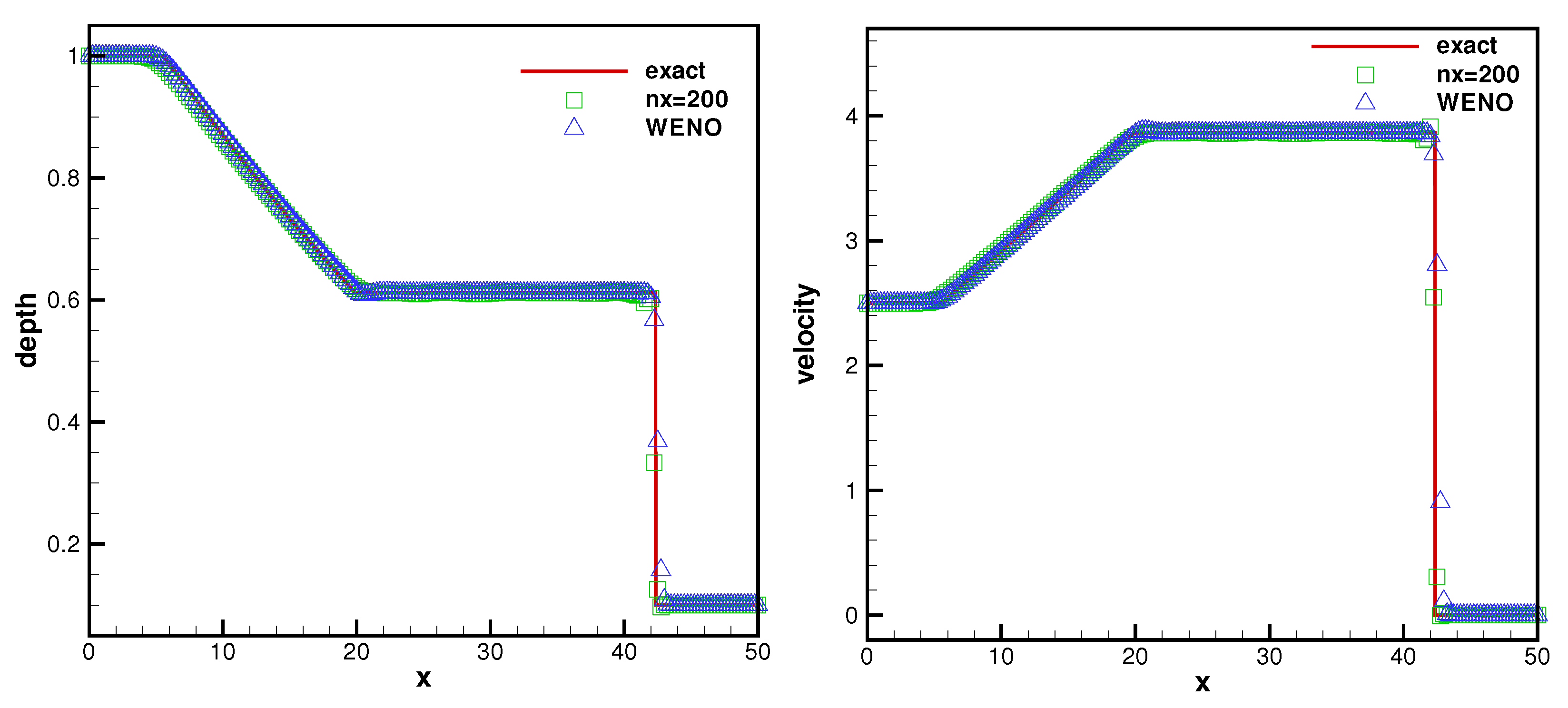
4.1. The SWEs

4.1.1. Example 1

The initial data of the first example is as follows

$$(h,u)(x,0)=\left\{\begin{array}{cc}(1,2.5),\hfill & \mathrm{if}0\le x\le 10,\hfill \\ (0.1,0),\hfill & \mathrm{otherwise},\hfill \end{array}\right.$$

on a domain $[0,50]$. Figure 1 shows the solutions at $t=7$ on a mesh with 200 cells.

Figure 1. The depth h (left) and the velocity u (right) of the water in Example 1.

The numerical solutions are all well resolved and fit well with the exact results. In addition, the results fit well with the results by the WENO schemes.

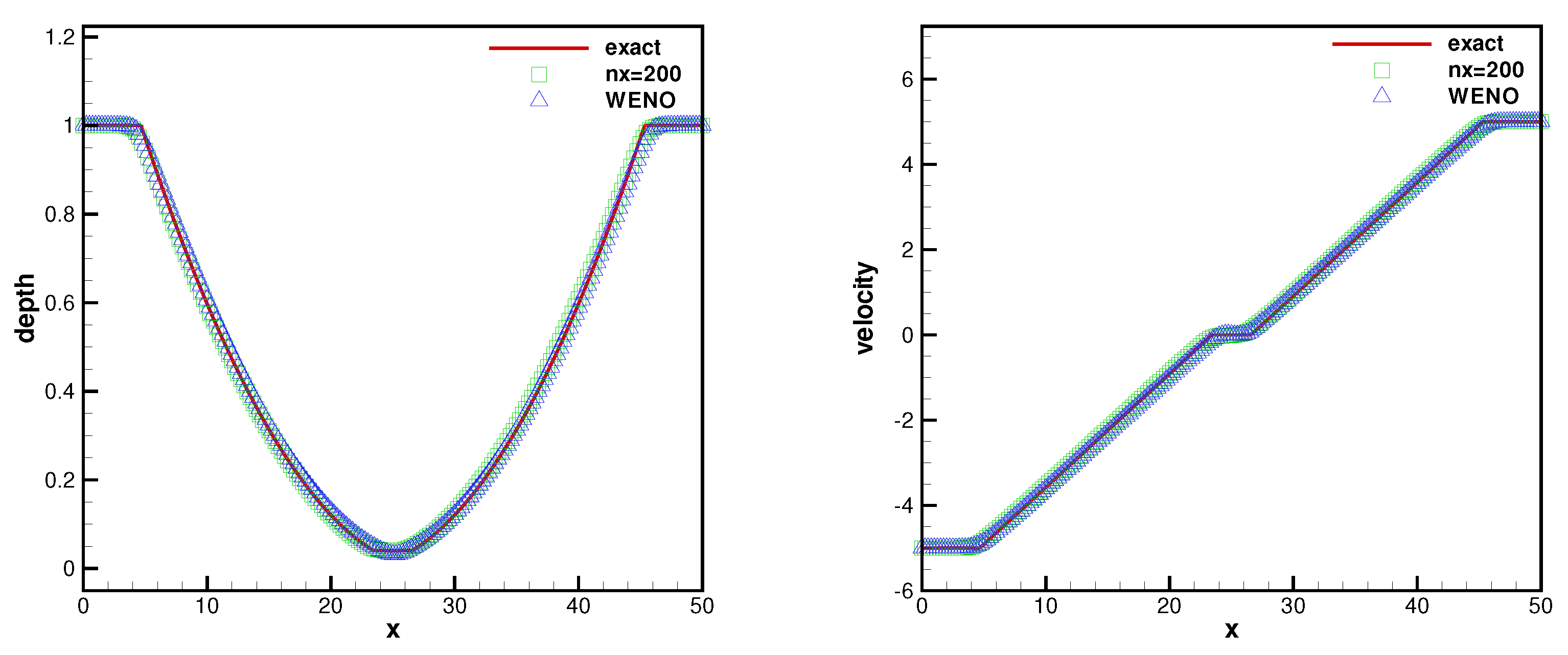
4.1.2. Example 2

For the second example, we apply the following data

$$\begin{array}{cc}\hfill (h,u)(x,0)& =\left\{\begin{array}{cc}(1,0),\hfill & \mathrm{if}0\le x\le 1000,\hfill \\ (0.5,0),\hfill & \mathrm{otherwise},\hfill \end{array}\right.\hfill \end{array}$$

on a domain $[0,2000]$. Figure 2 presents the numerical solutions at $t=240$.

Figure 2. The depth h (left) and the velocity u (right) of the water in Example 2.

Clearly, the current scheme produces well resolved solutions, which fit well with the exact solutions.

4.1.3. Example 3

Further, we adopt the following data

$$(h,u)(x,0)=\left\{\begin{array}{cc}\left(1,-5\right),\hfill & \mathrm{if}0\le x\le 25,\hfill \\ (1,5),\hfill & \mathrm{otherwise},\hfill \end{array}\right.$$

on a domain $[0,50]$. We implement it on a grid with 200 cells and compute this example until $t=2.5$. Figure 3 presents the numerical solutions and indicates that the results fit well with the exact ones.

Figure 3. The depth h (left) and the velocity u (right) of the water in Example 3.

4.1.4. Example 4

Subsequently, we deal with a dam break example using the following data

$$(h,u)(x,0)=\left\{\begin{array}{cc}\left(1,0\right),\hfill & \mathrm{if}-1000\le x\le 0,\hfill \\ (0.5,0),\hfill & \mathrm{otherwise},\hfill \end{array}\right.$$

on a domain $[-1000,2000]$. Then, we solve it up to $t=240$ on a grid with 200 cells.

Figure 4 shows the numerical solutions and indicates that the results are clearly consistent with the exact ones.

Figure 4. The depth h (left) and the velocity u (right) of the water in Example 4.

4.1.5. Example 5: Circular Dam Break Problem

Here, we simulate a circular dam break problem [46] for the 2D SWEs. We use this problem to testify the ability of the current scheme to maintain cylindrical symmetry. The following data are used for calculation.

$$\begin{array}{cc}\hfill h& =\left\{\begin{array}{cc}10,\hfill & \mathrm{if}\sqrt{{(x-25)}^2+{(y-25)}^2}\le 11,\hfill \\ 1,\hfill & \mathrm{otherwise}.\hfill \end{array}\right.\hfill \\ \hfill u& =v=0.\hfill \end{array}$$

The domain is $[0,50]\times [0,50]$ with the outflow boundary conditions.

Figure 5 presents the results $t=0,0.2,0.4,0.6,0.8,1.0$ obtained on a mesh with $200\times 200$ cells, which shows that our ES scheme can well capture the wave structures.

Figure 5. The contours of the height h on a mesh with $200\times 200$ cells.

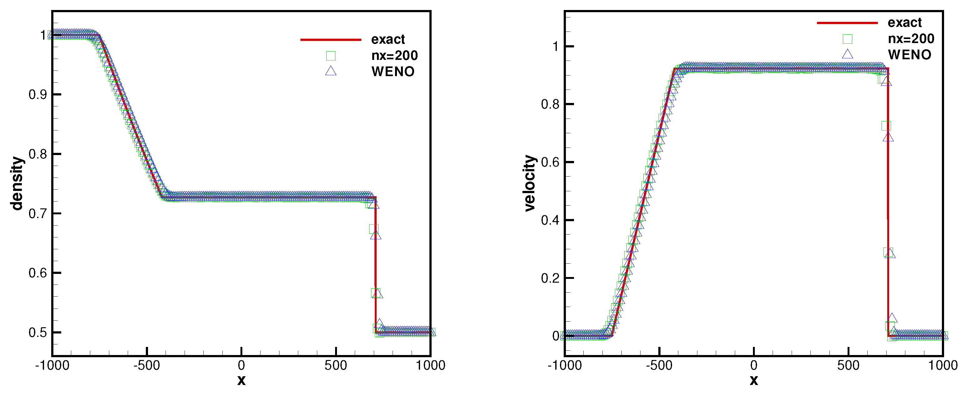
4.2. The Euler Equations of Gas Dynamics

4.2.1. Testing the Order of Accuracy

In order to demonstrate the order of accuracy, we take an example from [47].

$$\rho (x,t)=1+0.2sin\left(\pi \right(x-t\left)\right),u(x,t)=1,p(x,t)=1,x\in [0,2].$$

We apply periodic boundary conditions on both ends of the domain. Table 1 shows the errors at time $t=2$ and the orders of accuracy. It should be pointed out that we here take the step size of time as ${\displaystyle \Delta t=CFL\frac{{(\Delta x)}^{\frac{5}{3}}}{\alpha }}$ to keep the spatial errors dominant.

Table 1. The errors and orders of accuracy.

Cells	${\mathit{L}}^{\mathit{\infty }}\mathbf{Error}$	Order	${\mathit{L}}^1\mathbf{Error}$	Order	${\mathit{L}}^2\mathbf{Error}$	Order
25	7.1557 × 10${}^{-9}$		5.4250 × 10${}^{-9}$		4.6434 × 10${}^{-9}$
50	1.4620 × 10${}^{-9}$	2.29	5.0198 × 10${}^{-10}$	3.43	5.4977 × 10${}^{-10}$	3.08
100	3.2688 × 10${}^{-11}$	5.48	1.1626 × 10${}^{-11}$	5.43	1.2667 × 10${}^{-11}$	5.44
200	1.2699 × 10${}^{-12}$	4.69	5.8475 × 10${}^{-13}$	4.31	5.2894 × 10${}^{-13}$	4.58

4.2.2. Sod Problem

The initial data are as in [48]

$$(\rho ,u,p)(x,0)=\left\{\begin{array}{cc}(1,0,1)\hfill & \mathrm{if}x\le 0,\hfill \\ (0.125,0,0.1)\hfill & \mathrm{if}x>0,\hfill \end{array}\right.$$

on $[-5,5]$. Figure 6 shows the density at time $t=2$. Clearly, the contact discontinuities are well decomposed and the results maintain a steep discontinuity transition.

Figure 6. The density of the Sod problem at $t=2$.

4.2.3. Lax Problem

We use the following data

$$(\rho ,u,p)(x,0)=\left\{\begin{array}{cc}(0.445,0.698,3.528)\hfill & \mathrm{if}x\le 0,\hfill \\ (0.5,0,0.571)\hfill & \mathrm{if}x>0,\hfill \end{array}\right.$$

on $[-5,5]$. We can find a contact discontinuity that is hard to solve. Figure 7 shows the density at $t=1.3$ and makes a comparison with the exact one.

Figure 7. The density of the Lax problem at $t=1.3$.

4.2.4. Shu–Osher Problem

We adopt the initial data from [49]

$$\begin{array}{c}\hfill (\rho ,u,p)(x,0)=\left\{\begin{array}{cc}(3.857143,2.629369,10.333333)\hfill & \mathrm{if}x<-4,\hfill \\ (1+0.2sin(5x),0,1)\hfill & \mathrm{if}x\ge -4,\hfill \end{array}\right.\end{array}$$

on a domain $[-5,5]$. A shock is produced and it interacts with the smooth regions. Figure 8 presents the density at time $t=1.8$.

Figure 8. The density of the Shu-Osher problem at $t=1.8$.

4.2.5. 123 Problem

The data are given by [50]

$$(\rho ,u,p)(x,0)=\left\{\begin{array}{cc}(1,-2,0.4)\hfill & \mathrm{if}x<0.5,\hfill \\ (1,2,0.4)\hfill & \mathrm{if}x>0.5,\hfill \end{array}\right.$$

on $[0,1]$. Figure 9 shows the density at time $t=0.15$. It is clear that the new scheme can adequately resolve the central expansion regions.

Figure 9. The density of the 123 problem at $t=0.15$.

4.2.6. Modified Shock/Turbulence Interaction

We conduct an example [51] that is actually a modification of the shock/turbulence problem developed in [52,53]. The initial conditions are as follows

$$(\rho ,u,p)(x,0)=\left\{\begin{array}{cc}(1.515695,0.523346,1.805)\hfill & \mathrm{if}x\le -4.5,\hfill \\ \left(1+0.1sin\left(20\pi x\right),0,1\right)\hfill & \mathrm{if}x>-4.5,\hfill \end{array}\right.$$

on a domain $[-5,5]$. Using a mesh with 1000 cells, Figure 10 shows the density at time $t=5$. Both schemes provide exceptional resolution for oscillations.

Figure 10. The density of the modified shock/turbulence interaction problem at $t=5$.

5. Conclusions

This article proposes a high-order accurate ES finite difference scheme for nonlinear hyperbolic systems of conservation laws. This article mainly contains two innovative points: on one hand, a high-order accurate EC scheme is achieved by building the second-order EC schemes; on the other hand, the WENO reconstruction is employed based on the scaled entropy variables to obtain the high-order dissipation term. Furthermore, extensive results illustrate that the proposed scheme enjoys steep discontinuous transitions and keeps high-order accuracy. The current scheme can only be applied to uniform meshes or smooth transformed curve meshes for two-dimensional cases. In future research, we aim to expand the proposed scheme to uniform meshes.

References

- Bradford, S.F.; Sanders, B.F. Finite volume model for shallow water flooding of arbitrary topography. J. Hydraul. Eng. 2002, 128, 289–298. [Google Scholar] [CrossRef]
- Gottardi, G.; Venutelli, M. Central scheme for the two-dimensional dam-break flow simulation. Adv. Water Resour. 2004, 27, 259–268. [Google Scholar] [CrossRef]
- Vreugdenhil, C.B. Numerical Methods for Shallow-Water Flow; Springer: Dordrecht, The Netherlands, 1995; pp. 15–25. [Google Scholar]
- Perthame, B.; Simeoni, C. A kinetic scheme for the Saint-Venant system with a source term. Calcolo 2001, 38, 201–231. [Google Scholar] [CrossRef]
- Xu, K. A well-balanced gas-kinetic scheme for the shallow-water equations with source terms. J. Comput. Phys. 2002, 178, 533–562. [Google Scholar] [CrossRef]
- Kurganov, A.; Levy, D. Central-upwind schemes for the Saint-Venant system. Math. Model. Numer. Anal. 2002, 36, 397–425. [Google Scholar] [CrossRef]
- Vukovic, S.; Sopta, L. ENO and WENO schemes with the exact conservation property for one-dimensional shallow water equations. J. Comput. Phys. 2002, 179, 593–621. [Google Scholar] [CrossRef]
- Vukovic, S.; Crnjaric-Zic, N.; Sopta, L. WENO schemes for balance laws with spatially varying flux. J. Comput. Phys. 2004, 199, 87–109. [Google Scholar] [CrossRef]
- Xing, Y.L.; Shu, C.-W. High order finite difference WENO schemes with the exact conservation property for the shallow water equations. J. Comput. Phys. 2005, 208, 206–227. [Google Scholar] [CrossRef]
- Noelle, S.; Pankratz, N.; Puppo, G.; Natvig, J. Well-balanced finite volume schemes of arbitrary order of accuracy for shallow water flows. J. Comput. Phys. 2006, 213, 474–499. [Google Scholar] [CrossRef]
- Xing, Y.L.; Shu, C.-W. High order well-balanced finite volume WENO schemes and discontinuous Galerkin methods for a class of hyperbolic systems with source terms. J. Comput. Phys. 2006, 214, 567–598. [Google Scholar] [CrossRef]
- Noelle, S.; Xing, Y.; Shu, C.-W. High-order well-balanced finite volume WENO schemes for shallow water equation with moving water. J. Comput. Phys. 2007, 226, 29–58. [Google Scholar] [CrossRef]
- Li, G.; Lu, C.; Qiu, J. Hybrid well-balanced WENO schemes with different indicators for shallow water equations. J. Sci. Comput. 2012, 51, 527–559. [Google Scholar] [CrossRef]
- Li, G.; Caleffi, V.; Qi, Z.K. A well-balanced finite difference WENO scheme for shallow water flow model. Appl. Math. Comput. 2015, 265, 1–16. [Google Scholar] [CrossRef]
- Zhu, Q.; Gao, Z.; Don, W.S.; Lv, X. Well-balanced hybrid compact-WENO scheme for shallow water equations. Appl. Numer. Math. 2017, 112, 65–78. [Google Scholar] [CrossRef]
- Li, J.J.; Li, G.; Qian, S.G.; Gao, J.M. High-order well-balanced finite volume WENO schemes with conservative variables decomposition for shallow water equations. Adv. Appl. Math. Mech. 2021, 13, 827–849. [Google Scholar]
- Caleffi, V. A new well-balanced Hermite weighted essentially non-oscillatory scheme for shallow water equations. Int. J. Numer. Methods Fluids 2011, 67, 1135–1159. [Google Scholar] [CrossRef]
- Russo, G. Central schemes for balance laws. In Proceedings of the VIII International Conference on Nonlinear Hyperbolic Problems, Magdeburg, Germany, 28 February–3 March 2000. [Google Scholar]
- Touma, R.; Khankan, S. Well-balanced unstaggered central schemes for one and two-dimensional shallow water equation systems. Appl. Math. Comput. 2012, 218, 5948–5960. [Google Scholar] [CrossRef]
- Ern, A.; Piperno, S.; Djadel, K. A well-balanced Runge-Kutta discontinuous Galerkin method for the shallow-water equations with flooding and drying. Int. J. Numer. Methods Fluids 2008, 58, 1–25. [Google Scholar] [CrossRef]
- Xing, Y. Exactly well-balanced discontinuous Galerkin methods for the shallow water equations with moving water equilibrium. J. Comput. Phys. 2014, 257, 536–553. [Google Scholar] [CrossRef]
- Li, G.; Song, L.N.; Gao, J.M. High order well-balanced discontinuous Galerkin methods based on hydrostatic reconstruction for shallow water equations. J. Comput. Appl. Math. 2018, 340, 546–560. [Google Scholar] [CrossRef]
- Vignoli, G.; Titarev, V.A.; Toro, E.F. ADER schemes for the shallow water equations in channel with irregular bottom elevation. J. Comput. 2008, 227, 2463–2480. [Google Scholar] [CrossRef]
- Navas-Montilla, A.; Murillo, J. Energy balanced numerical schemes with very high order. The Augmented Roe Flux ADER scheme. Application to the shallow water equations. J. Comput. Phys. 2015, 290, 188–218. [Google Scholar] [CrossRef]
- Gassner, G.J.; Winters, A.R.; Kopriva, D.A. A well balanced and entropy conservative discontinuous Galerkin spectral element method for the shallow water equations. Appl. Math. Comput. 2016, 272, 291–308. [Google Scholar] [CrossRef]
- Berthon, C.; Chalons, C. A fully well-balanced, positive and entropy-satisfying Godunov-type method for the shallow-water equations. Math. Comput. 2016, 85, 1281–1307. [Google Scholar] [CrossRef]
- Yuan, X.H. A well-balanced element-free Galerkin method for the nonlinear shallow water equations. Appl. Math. Comput. 2018, 331, 46–53. [Google Scholar] [CrossRef]
- Li, G.; Li, J.J.; Qian, S.G.; Gao, J.M. A well-balanced ADER discontinuous Galerkin method based on differential transformation procedure for shallow water equations. Appl. Math. Comput. 2021, 395, 125848. [Google Scholar] [CrossRef]
- Liu, Y.Y.; Yang, L.M.; Shu, C.; Zhang, H.W. Three-dimensional high-order least square-based finite difference-finite volume method on unstructured grids. Phys. Fluids 2020, 32, 123604. [Google Scholar] [CrossRef]
- Liu, Y.Y.; Shu, C.; Yang, L.M.; Liu, Y.G.; Liu, W.; Zhang, Z.L. High-order implicit RBF-based differential quadrature-finite volume method on unstructured grids: Application to inviscid and viscous compressible flows. J. Comput. Phys. 2023, 478, 111962. [Google Scholar] [CrossRef]
- Jitendra; Chaurasiya, V.; Rai, K.N.; Singh, J. Legendre wavelet residual approach for moving boundary problem with variable thermal physical properties. Int. J. Nonlinear Sci. Numer. Simul. 2022, 23, 947–956. [Google Scholar]
- Chaurasiya, V.; Jain, A.; Singh, J. Numerical study of a non-linear porous sublimation problem with temperature-dependent thermal conductivity and Concentration-Dependent Mass Diffusivity. ASME J. Heat Mass Transf. 2023, 145, 072701. [Google Scholar] [CrossRef]
- Chaudhary, R.K.; Chaurasiya, V.; Singh, J. Numerical estimation of temperature response with step heating of a multi-layer skin under the generalized boundary condition. J. Therm. Biol. 2022, 108, 103278. [Google Scholar] [CrossRef]
- Fjordholm, U.S.; Mishra, S.; Tadmor, E. The numerical viscosity of entropy stable schemes for systems of conservation laws. I. Math. Comput. 1987, 49, 91–103. [Google Scholar]
- Duan, J.M.; Tang, H.Z. High-order accurate entropy stable finite difference schemes for the shallow water magneto-hydrodynamics. J. Comput. Phys. 2021, 431, 110136. [Google Scholar] [CrossRef]
- Winters, A.R.; Gassner, G.J. A comparison of two entropy stable discontinuous Galerkin spectral element approximations for the shallow water equations with non-constant topography Author links open overlay panel. J. Comput. Phys. 2015, 301, 357–376. [Google Scholar] [CrossRef]
- Wintermeyer, N.; Winters, A.R.; Gassner, G.J.; Kopriva, D.A. An entropy stable nodal discontinuous Galerkin method for the two dimensional shallow water equations on unstructured curvilinear meshes with discontinuous bathymetry. J. Comput. Phys. 2017, 340, 200–242. [Google Scholar] [CrossRef]
- Wintermeyer, N.; Winters, A.R.; Gassner, G.J.; Warburton, T. An entropy stable discontinuous Galerkin method for the shallow water equations on curvilinear meshes with wet/dry fronts accelerated by GPUs. J. Comput. Phys. 2018, 375, 447–480. [Google Scholar] [CrossRef]
- Wen, X.; Don, W.S.; Gao, Z.; Xing, Y.L. Entropy stable and well-balanced discontinuous Galerkin methods for the nonlinear shallow water equations. J. Sci. Comput. 2020, 83, 66. [Google Scholar] [CrossRef]
- Liu, Q.S.; Liu, Y.Q.; Feng, J.H. The scaled entropy variables reconstruction for entropy stable schemes with application to shallow water equations. Comput. Fluids 2019, 192, 104266. [Google Scholar] [CrossRef]
- Ismail, F.; Roe, P.L. Affordable, entropy-consistent Euler flux functions II: Entropy production at shocks. J. Comput. Phys. 2009, 228, 5410–5436. [Google Scholar] [CrossRef]
- Lefloch, P.G.; Mercier, J.M.; Rohde, C. Fully discrete entropy conservative schemes of arbitrary order. SIAM J. Numer. Anal. 2002, 40, 1968–1992. [Google Scholar] [CrossRef]
- Fjordholm, U.S.; Mishra, S.; Tadmor, E. Arbitrarily high-order accurate entropy stable essentially non-oscillatory schemes for systems of conservation laws. SIAM J. Numer. Anal. 2012, 50, 544–573. [Google Scholar] [CrossRef]
- Fjordholm, U.S.; Mishra, S.; Tadmor, E. ENO reconstruction and ENO interpolation are stable. Found. Comput. Math. 2013, 13, 139–159. [Google Scholar] [CrossRef]
- Biswas, B.; Dubey, R.K. Low dissipative entropy stable schemes using third order WENO and TVD reconstructions. Adv. Comput. Math. 2018, 44, 1153–1181. [Google Scholar] [CrossRef]
- Alcrudo, F.; Garcia-Navarro, P. A high-resolution Godunov-type scheme in finite volumes for the 2D shallow-water equations. Int. J. Numer. Methods Fluids 1993, 16, 489–505. [Google Scholar] [CrossRef]
- Qiu, J.; Shu, C.-W. Hermite WENO schemes and their application as limiters for Runge–Kutta discontinuous Galerkin method: One-dimensional case. J. Comput. Phys. 2003, 193, 115–135. [Google Scholar] [CrossRef]
- Sod, G. A survey of several finite difference methods for systems of nonlinear hyperbolic conservation laws. J. Comput. Phys. 1978, 27, 1–31. [Google Scholar] [CrossRef]
- Shu, C.-W.; Osher, S. Efficient implementation of essentially non-oscillatory shock capturing schemes. J. Comput. Phys. 1988, 77, 439–471. [Google Scholar] [CrossRef]
- Toro, E.F. Riemann Solvers and Numerical Methods for Fluid Dynamics: A Practical Introduction; Springer: Berlin/Heidelberg, Germany, 1999. [Google Scholar]
- Toro, E.F.; Titarev, V.A. TVD fluxes for the high-order ADER schemes. J. Sci. Comput. 2005, 24, 285–309. [Google Scholar] [CrossRef]
- Jiang, G.S.; Shu, C.-W. Efficient Implementation of weighted ENO Schemes. J. Comput. Phys. 1996, 126, 202–228. [Google Scholar] [CrossRef]
- Balsara, D.S.; Shu, C.-W. Monotonicity preserving weighted essentially non-oscillatory schemes with increasingly high order of accuracy. J. Comput. Phys. 2000, 160, 405–452. [Google Scholar] [CrossRef]