Abstract
This research aims to propose a new family of one-parameter multi-step iterative methods that combine the homotopy perturbation method with a quadrature formula for solving nonlinear equations. The proposed methods are based on a higher-order convergence scheme that allows for faster and more efficient convergence compared to existing methods. It aims also to demonstrate that the efficiency index of the proposed iterative methods can reach up to and , respectively, indicating a high degree of accuracy and efficiency in solving nonlinear equations. To evaluate the effectiveness of the suggested methods, several numerical examples including their performance are provided and compared with existing methods.
MSC:
65H05; 65B99
1. Introduction
Nonlinear equations are ubiquitous in various scientific and engineering fields and are of great importance in applied mathematics. Finding their solutions analytically is often infeasible or impossible, and therefore numerical iterative methods are commonly employed to obtain approximations. Among the classical iterative formulas, Newton’s method and its variants are widely used, but many other techniques have been developed and studied, such as the Adomian decomposition method, the variational iteration method, and the differential transform method, to name a few (see [1,2,3,4,5] and the references therein).
One of the techniques that has gained attention for obtaining iterative methods for nonlinear equations is the homotopy analysis method (HAM) introduced by Liao in 1992 [6]. Another successful iterative method for nonlinear equations is the homotopy perturbation method (HPM), which is a special case of HAM introduced by He in 1999 [7] (see [8,9,10] for more details). Since then, many developments and extensions of HPM have been proposed by many authors, such as Sehati et al. [11] and others, resulting in a variety of novel iterative methods with higher orders of convergence. For instance, Waheed et al. [12] used the HPM to develop certain iterative methods with high accuracy and efficiency.
Recent advances in artificial intelligence and machine learning techniques have also been applied to develop iterative methods for nonlinear equations, such as using deep learning neural networks, for predicting iterative solutions [13,14].
An essential aspect of iterative methods is their convergence rate, which determines how quickly the method converges to the true solution. Numerous studies have focused on the convergence analysis of iterative methods for nonlinear equations, resulting in various convergence criteria that can be used to improve the efficiency of iterative methods and optimize their convergence rate [11,15,16,17].
Iterative methods for solving nonlinear equations are a vital research area with many practical applications. The recent developments in this field, including the use of the HPM and artificial intelligence techniques, have expanded the available toolkit for approximating the solutions of nonlinear equations and have led to improved insights into their behavior. As research in this area continues, further advances can be expected in the accuracy and efficiency of iterative methods, enabling researchers to tackle increasingly complex nonlinear problems.
Motivated by the objective of enhancing the precision and efficiency of iterative methods employed in solving nonlinear equations, this paper introduces a novel multi-step iterative method that combines the Haar wavelets quadrature formula and the homotopy perturbation technique. The organization of the paper is as follows: Section 2 presents the construction of the new iterative methods, comprising a novel set of algorithms designed specifically for solving nonlinear equations. The algorithms employed as proposed methods are demonstrated, accompanied by an explanation of their underlying rationale. Section 3 provides a convergence analysis of the proposed methods, accompanied by the declaration of efficiency indices. The performance of the algorithms is further assessed through an analysis of convergence rates. Additionally, efficiency indices, which serve as indicators of the computational cost and accuracy of the methods, are described. In Section 4, a comparative analysis is conducted between the performance of the proposed algorithms and several existing methods found in the literature. Various examples are employed to evaluate the performance of the algorithms, and numerical results are presented to demonstrate their effectiveness in solving the problem at hand. Furthermore, graphical representations are utilized to provide a more comprehensive description of the convergence, accuracy, and reliability of the proposed algorithms. Lastly, Section 5 delves into a discussion of the obtained results, drawing conclusions from the analysis conducted. The strengths and weaknesses of the proposed methods are highlighted, and suggestions for future research directions are provided.
2. The New Iterative Methods Construction
Consider the following nonlinear equation:
and suppose be a simple root of Equation (1), and is an initial approximation near to . Consider the quadrature formula which is defined by
Approximating the above integral in Equation (2) by using Haar wavelets quadrature formula [18], one could obtain that
Assuming that is close enough to in Equation (3) leads to
Based on HPM, the construction of the homotopy can be made, which will satisfy
where is an artificial parameter. As a trivial case, one could see that
and
The solution of Equation (5) is obtained as an infinite series that is given as
Consequently, the approximate solution of Equation (1) is given by
provided the series (8) converges. Series (9) is convergent for most cases, and also the rate of convergence depends on [7]. Equation (5) can be expressed as follows by using Taylor’s series [19] for and about :
Matching powers of the above coefficients of p, one can obtain the following system of equations
and so on. After solving the above system of equations, the following is obtained:
Substituting the values of and in (9) obtains
The above formula is a generalization of Equation (8) in [20]. From the aforementioned formulation, a one-step iterative method is presented for solving nonlinear equations, which is given by the following Algorithm 1.
| Algorithm 1: A suggested one-step iterative method. |
For a suitable initial approximation , calculate the next solution using the below iterative method
|
As the aim of this study is to develop effective multi-step iterative methods, we rely on Algorithm 1 and the following iterative method proposed by [17]:
where , and is selected such that the corresponding function value and have the same signs.
In addition, to improve the efficiency of the new iterative methods, the first and second derivatives and are approximated, respectively, by using a Bernoulli interpolating polynomial of degree 2 and as follows:
Furthermore, using the Bernoulli interpolating polynomial of degree 3, the derivative is approximated:
Therefore, the new two and three step iterative methods, which will be referred to as (HM2) and (HM3), respectively, are given by the following Algorithms 2 and 3:
| Algorithm 2: A suggested two-step iterative method (HM2). |
For a suitable initial approximation , calculate the next solution using the following iterative method: |
| Algorithm 3: A suggested three-step iterative method (HM3). |
For a suitable initial approximation , calculate the next solution using the following iterative method: |
3. Convergence Investigation
In this section, a convergence analysis of Algorithms 2 and 3 is provided and their efficiency indices are stated. Specifically, it is meant to show that both algorithms converge to the exact solution of the nonlinear equation under certain conditions on the initial guess and the nonlinear function. Moreover, the convergence rate of the proposed iterative methods is analyzed by computing their efficiency indices, which reflect the number of iterations required to achieve a given level of accuracy.
Theorem 1.
Suppose that is a smooth function with a simple root . If is sufficiently near to α, then Algorithm 2 exhibits at least fourth-order convergence in its iteration towards the exact root.
Proof.
Let be a simple root of . (Note that, and . By applying the Taylor series expansion around , one can expand and to obtain the following:
where and . From Equation (17), it can be shown that
and hence,
Moreover,
From Equation (20), it can be seen that
In addition,
and
Substituting Equations (24)–(27) in Algorithm 2 obtains
implying that
As a result, it can be seen that Algorithm 2 has fourth-order convergence. □
Theorem 2.
Suppose that is a smooth function with a simple root . If is sufficiently near to α, then Algorithm 3 exhibits at least eighth-order convergence in its iteration towards the exact root.
Proof.
In fact, it is essential in numerical analysis to know the behavior of an approximate method. Therefore, the order of convergence of the new iterative methods can be explained by the following definition and remark (more details can be found in [11,21,22]).
Definition 1.
Let is a scalar function on an open interval D with a simple root α of the nonlinear equation. An iterative method is said to have an integer order of convergence s if it produces the sequence of real numbers such that
for some and , then s is said to be the order of convergence of the sequence, and A is known as the asymptotic error constant, or equivalently
Remark 1.
Let be the error in the iteration. The equation
is called the error equation for the method, s being the order of convergence.
Remark 2.
The definition of efficiency index in [16] is analyzed, which is given as , where s is the order of the iterative method and m is the number of function evaluations in each iteration. Using this definition, the efficiency indices of our suggested Algorithms 2 and 3 are 1.587 and 1.681, respectively.
4. Numerical Applications
The purpose of this section is to compare the performance of the proposed Algorithms 2 and 3 with the Noor method (NR2) [2], the Chun method (CM) [23], and the Sehati et al. method (AL2) [11]. The comparison is aimed at demonstrating the applicability and efficacy of the newly proposed methods.
To evaluate the methods, the Maple16 program is utilized and floating-point arithmetic with 1000 digits (Digits := 1000) is employed. The computations were performed on a desktop machine that runs on Windows 10 Pro (64-bit) operating system. The computer is equipped with an Intel(R) Core(TM) i3-4170 CPU that runs at a speed of GHz, and it has a total installed memory of 10.00 GB RAM. The system configuration provided ample resources to ensure a smooth and efficient execution of the Maple16 algorithms used in this study. The stopping criteria as well as are used, where , and (HM2) and (HM3) have been applied for the value of . Table 1 presents various test functions , and the approximated root of each equation . The table also provides information about the initial guess , the number of iterations , the value of , the absolute value of the function , and the computational order of convergence (COC) , which is described in [16] and given as the following:
All the results and the performance comparison are included in Table 2.

Table 1.
Nonlinear equations and their simple root .
Table 2.
Comparison between the proposed methods and relevant methods.
Moreover, Figure 1, Figure 2, Figure 3, Figure 4 and Figure 5 are presented to provide a more comprehensive description of the convergence, accuracy, and reliability of the proposed Algorithms 2 and 3. These graphs display the logarithm of residuals at each iteration for the nonlinear equations listed in Table 1. Additionally, Figure 6 is included, which compares the efficiency of the suggested two- and three-step methods with the alternative methods that have been considered.
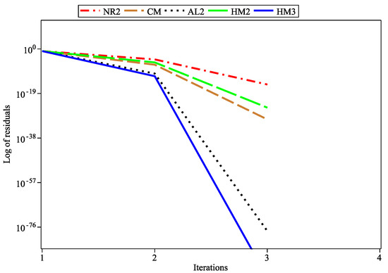
Figure 1.
Log of residuals for .
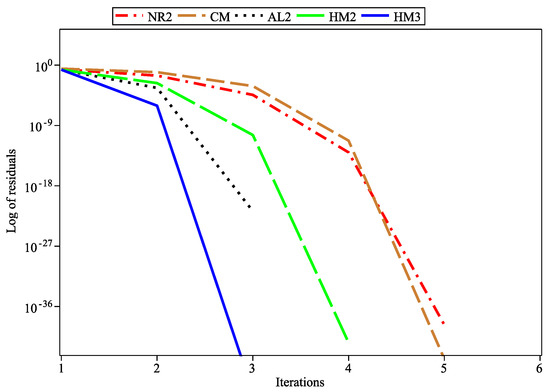
Figure 2.
Log of residuals for .
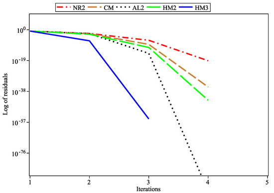
Figure 3.
Log of residuals for .
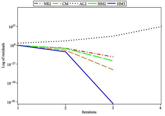
Figure 4.
Log of residuals for .
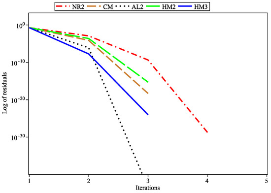
Figure 5.
Log of residuals for .
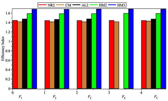
Figure 6.
Comparison of efficiency indices among different methods.
5. Discussion and Conclusions
The numerical findings in Table 2 and Figure 1, Figure 2, Figure 3, Figure 4 and Figure 5 demonstrate that none of the five nonlinear equations above exhibits the failure or divergence of our multi-step iterative methods. The new three-step iterative method proves to be more effective and accurate, and provides solutions faster than the other methods that it is compared against, such as Noor’s method, Chun’s method, and the Sehati et al. method. Moreover, the suggested iterative methods have a higher computational order of convergence (COC) than any other methods, making them more efficient. Our findings can be viewed as an alternative to comparable methods for solving nonlinear equations as they approximate higher derivatives, enabling us to obtain solutions with fewer computational steps and a higher order of convergence.
This paper introduces a new class of iterative methods free from second derivatives to solve nonlinear equations based on the homotopy perturbation method, Haar wavelets quadrature rule, and some numerical techniques. The suggested iterative methods have a fourth-order convergence for the two-step type with two function evaluations and one first derivative evaluation, while for the three-step type, it has an eighth-order convergence with three function evaluations and one first derivative evaluation. The convergence order using Theorems 1 and 2, efficiency index, computational order of convergence, and convergence criterion of the new multi-step iterative methods are evaluated. The proposed Algorithms 2 and 3 outperform the previously mentioned methods in terms of efficiency index. The eighth-order iterative method (HM3) is the key finding of this study since it is both fast and efficient, as evident through both theoretical evaluation and numerical testing.
The suggested methods are numerically and graphically compared to several currently used methods, and the proposed methods outperform several other previously known methods in terms of convergence rate and computational efficiency. The obtained results show that the proposed methods are promising tools for solving nonlinear equations, as they outperform existing methods. Overall, our work provides a novel approach to solving nonlinear equations that can significantly improve the accuracy and efficiency of numerical methods, indicating its potential for use in a range of scientific and engineering applications.
There are several potential directions for future work. For instance, hybrid algorithms that combine the proposed methods with other existing techniques could be developed to further improve their performance. Additionally, more efficient and accurate versions of the methods could be created to enhance their effectiveness. Furthermore, the methods can be adapted or modified to tackle more complex and diverse problems, including systems of nonlinear equations.
Author Contributions
Conceptualization, H.J.S. and A.H.A.; Methodology, H.J.S. and A.H.A.; Software, A.H.A. and H.A.; Validation, A.D.P.; Formal analysis, R.M.; Investigation, R.M.; Resources, R.M.; Data curation, H.J.S.; Writing—original draft, H.J.S. and R.M.; Writing—review & editing, A.H.A., A.D.P. and H.A.; Visualization, A.H.A. and H.A.; Supervision, A.D.P.; Project administration, A.D.P.; Funding acquisition, A.D.P. All authors have read and agreed to the published version of the manuscript.
Funding
The authors did not receive any funding to support this study.
Institutional Review Board Statement
Not applicable.
Informed Consent Statement
Not applicable.
Data Availability Statement
No data were used for this work.
Conflicts of Interest
The authors declare that they have no competing interest.
References
- Noor, K.I.; Noor, M.A. Predictor-corrector Hally method for nonlinear equations. Appl. Math. Comput. 2007, 188, 1587–1591. [Google Scholar]
- Noor, M.A.; Noor, K.I.; Mohyud-Din, S.T.; Shabbir, A. An iterative method with cubic convergence for nonlinear equations. Appl. Math. Comput. 2006, 183, 1249–1255. [Google Scholar] [CrossRef]
- Noor, M.A. Some iterative methods for solving nonlinear equations using homotopy perturbation method. Int. J. Comput. Math. 2010, 1, 141149. [Google Scholar] [CrossRef]
- Noor, M.A.; Khan, W.A. New iterative methods for solving nonlinear equation by using homotopy perturbation method. Appl. Math. Comput. 2012, 219, 3565–3574. [Google Scholar] [CrossRef]
- Abdul-Hassan, N.Y.; Ali, A.H.; Park, C. A new fifth-order iterative method free from second derivative for solving nonlinear equations. J. Appl. Math. Comput. 2022, 68, 2877–2886. [Google Scholar] [CrossRef]
- Liao, S.J. The Proposed Homotopy Analysis Technique for the Solution of Nonlinear Problems. Ph.D. Thesis, Shanghai Jiao Tong University, Shanghai, China, 1992. [Google Scholar]
- He, J.H. Homotopy perturbation technique. Comput. Methods Appl. Mech. Eng. 1999, 178, 257–262. [Google Scholar] [CrossRef]
- Liao, S.J. Comparison between the homotopy analysis method and homotopy perturbation method. Appl. Math. Comput. 2005, 169, 1186–1194. [Google Scholar] [CrossRef]
- Az-Zo’bi, E.A.; Al-Khaled, K.; Darweesh, A. Numeric-analytic solutions for nonlinear oscillators via the modified multi-stage decomposition method. Mathematics 2019, 7, 550. [Google Scholar] [CrossRef]
- Alim, M.A.; Kawser, M.A. Illustration of the homotopy perturbation method to the modified nonlinear single degree of freedom system. Chaos Solitons Fractals 2023, 171, 113481. [Google Scholar] [CrossRef]
- Sehati, M.M.; Karbassi, S.M.; Heydari, M.; Loghmani, G.B. several new iterative methods for solving nonlinear algebraic equations incorporating homotopy perturbation method (HPM). Int. J. Phys. Sci. 2012, 12, 5017–5025. [Google Scholar] [CrossRef]
- Waheed, A.; Din, S.T.M.; Zeb, M.; Usman, M. Some Higher Order Algorithms for Solving Fixed Point Problems. Commun. Math. Appl. 2018, 1, 41–52. [Google Scholar]
- Freno, B.A.; Carlberg, T.K. Machine-learning error models for approximate solutions to parameterized systems of nonlinear equations. Comput. Methods Appl. Mech. Eng. 2019, 348, 250–296. [Google Scholar] [CrossRef]
- Gong, W.; Liao, Z.; Mi, X.; Wang, L.; Guo, Y. Nonlinear equations solving with intelligent optimization algorithms: A survey. Complex Syst. Model. Simul. 2021, 1, 15–32. [Google Scholar] [CrossRef]
- Abbasbandy, S. Improving Newton-Raphson method for nonlinear equations by modified Adomian decomposition method. Appl. Math. Comput. 2023, 145, 887–893. [Google Scholar] [CrossRef]
- Saeed, H.J.; Abdul-Hassan, N.Y. An Efficient Three-Step Iterative Methods Based on Bernstein Quadrature Formula for Solving Nonlinear Equations. Basrah J. Sci. 2021, 3, 355–383. [Google Scholar] [CrossRef]
- Wu, X.Y. A New Continuation Newton-Like Method and its Deformation. Appl. Math. Comput. 2000, 112, 75–78. [Google Scholar] [CrossRef]
- Aziz, I.; Siraj-ul-Islam; Khan, W. Quadrature Rules for Numerical Integration Based on Haar wavelets and Hybrid Functions. Comput. Math. Appl. 2011, 61, 2770–2781. [Google Scholar] [CrossRef]
- Ali, A.H.; Páles, Z. Taylor-type Expansions in Terms of Exponential Polynomials. Math. Inequalities Appl. 2022, 25, 1123–1141. [Google Scholar] [CrossRef]
- Abbasbandy, S. Modified homotopy perturbation method for nonlinear equations and comparison with Adomian decomposition method. Appl. Math. Comput. 2006, 172, 431–438. [Google Scholar] [CrossRef]
- Ljajko, E.; Tosic, M.; Kevkic, T.; Stojanovic, V. Application of the Homotopy Perturbations Method in Approximation Probability Distributions of Non-linear Time Series. Univ. Politeh. Buchar. Sci.-Bull.-Ser.-Appl. Math. Phys. 2021, 83, 177–186. [Google Scholar]
- Khan, K.; Syed, H.Z. Semi Analytic Solution of Hodgkin-Huxley Model by Homotopy Perturbation Method. Punjab Univ. J. Math. 2021, 53, 825–842. [Google Scholar] [CrossRef]
- Chun, C. A new iterative method for solving nonlinear equations. Appl. Math. Comput. 2006, 178, 415–422. [Google Scholar] [CrossRef]
Disclaimer/Publisher’s Note: The statements, opinions and data contained in all publications are solely those of the individual author(s) and contributor(s) and not of MDPI and/or the editor(s). MDPI and/or the editor(s) disclaim responsibility for any injury to people or property resulting from any ideas, methods, instructions or products referred to in the content. |
© 2023 by the authors. Licensee MDPI, Basel, Switzerland. This article is an open access article distributed under the terms and conditions of the Creative Commons Attribution (CC BY) license (https://creativecommons.org/licenses/by/4.0/).