Equivalent-Input-Disturbance Based Robust Control Design for Fuzzy Semi-Markovian Jump Systems via the Proportional-Integral Observer Approach

Abstract

This work focuses on the design of a unified control law, which enhances the accuracy of both the disturbance estimation and stabilization of nonlinear T-S fuzzy semi-Markovian jump systems. In detail, a proportional-integral observer based equivalent-input-disturbance (PIO-EID) approach is considered to model and develop the controller. The PIO approach includes a variable for relaxation in the system design along with an additional term for integration to improve the flexibility of the design and endurance of the system. The proposed stability criteria are formulated in the form of matrix inequalities using Lyapunov theory and depend on the sojourn time for robust control design. Final analyses are performed using MATLAB software with simulations to endorse the theoretical findings of this paper.

1. Introduction

In the real world, nonlinearity poses many challenges during the analysis of the stability and stabilization of control systems. The study based on the Takagi–Sugeno (T-S) fuzzy model technique has attracted a lot of attention due to its remarkable ability to approximate complex nonlinear systems as the weighted sum of linearized subsystems at operating points using fuzzy membership functions and if–then rules. In recent decades, remarkable research attention has been given to the stability and stabilization for T-S fuzzy systems [1,2,3,4,5,6]. In [7,8], the authors looked into the $H_{\infty }$ filtering problem for nonlinear switched systems with time-varying delay by incorporating T-S fuzzy model characteristics. The research findings in the design of fault-tolerant controller for fuzzy systems with actuator fault were presented in [3,9].

Meanwhile, random factors may also have an impact on physical systems that are actually in use, rapidly altering the structure of the system. Due to the fact that traditional systems are unable to accurately reflect the system models in this situation, MJSs are used to describe them. As a result of their composition as a collection of subsystems with Markov chains that select values from a finite set, MJSs are seen as an effective tool for modeling systems that are subject to rapid changes. To be specific, the sojourn time (ST) is the interval between two subsequent jumps. In reality, the ST of MJS is a random variable distributed according to a probability distribution, and the ${\epsilon }_{\iota \wp }\left(\mathfrak{l}\right)$ variable denotes the rate at which the system switches from mode i to mode j. The transition rate (TR) is usually taken to be constant, i.e., ${\epsilon }_{\iota \wp }\left(\mathfrak{l}\right)={\epsilon }_{\iota \wp }$. In particular, the ST of each subsystem in MJSs [10,11,12], however, is restricted to following an exponential distribution, leading to constant TRs, whereas, it can be challenging to guarantee some jump systems based on this presumption to have constant TR. Therefore, SMJS are introduced where the TR varies according to the ST. In contrast to MJSs, refs. [13,14,15,16] emphasized that the ST could follow more generic probability distributions. Therefore, compared to MJSs, SMJSs [17,18,19] have a wider range of practical application domains, and MJSs are thought to be more specific than SMJSs. Additionally, as the T-S fuzzy approach can simulate complex nonlinear systems, fuzzy model-based SMJSs [20,21] have also drawn a lot of attention. In [22,23], a sliding mode control for reliable stabilization in a class of continuous-time T-S fuzzy SMJSs with time delay was studied. Event-triggered control was devised for T-S fuzzy SMJSs in [24,25].

On the other hand, external disturbances in a system not only collapse the control performance but also result in malfunctions, vibrations, and other issues. Though fault tolerant control schemes themselves offer robust performance against matching external disturbance, they are unable to attenuate or, in certain cases, even amplify mismatch disturbances. A new area of study is the EID estimator, which calculates an equivalent disturbance on the control input to eliminate disturbances in the relevant control systems, which are not necessarily periodic, and they may be aperiodic in nature. In this regard, the literature [26,27,28,29,30,31,32] has provided a few intriguing results on the EID technique. To be specific, the Luenberger observer has a proportionate loop of the system output error and has significantly helped in the calculation of the EID. Compared with the Luenberger observer, the PIO, which increases the estimation accuracy of state variables with additional integral feedback to rebuild the state without previous knowledge of the system for estimating EID making the system robust, has been employed in the recent literature [33,34]. Numerous original and fascinating findings on the PIO for fuzzy systems have been made to date in [35,36]. The authors in [37] explored the disturbance rejection method for a linear control system based on the PIO and EID estimator. However, EID based control along with PIO for FSMJS has not been jointly investigated in the previous literature.

The above discussions shed light on this work, which concentrates on the stability and disturbance rejection issue of FSMJSs that are subject to actuator fault with parametric uncertainties. The bullet points listed below provide the major contributions made in this work:

• The EID based FSMJSs with a PIO are being taken into consideration for the first time.
• A new set of LMI-based restrictions is derived using Lyapunov functional approaches to ensure the disturbance rejection and stochastic stability of FSMJSs.
• The accompanying controller gain and observer gain are realized by addressing the LMI restrictions. The offered simulation results are able to unequivocally show the advantages and applicability of the produced theoretical conclusions.

The remainder of this article proceeds as follows: Section 2 illustrates the construction of an EID based FSMJS with a PIO. Through mathematical authentications, the major result is demonstrated in Section 3. The efficiency of the suggested control design is demonstrated by the theoretical findings in Section 4. Section 5 draws a brief conclusion regarding our study.

2. Problem Formulation and Preliminaries

Let us consider the following FSMJSs:

Plant rule $\varsigma$: If ${\Psi }_1\left(t\right)$ is ${{\rm Y}}_{\varsigma 1}$, ${\Psi }_2\left(t\right)$ is ${{\rm Y}}_{\varsigma 2}$, and ⋯${\Psi }_g\left(t\right)$ is ${{\rm Y}}_{\varsigma g}$, then:

$$\begin{array}{c}\hfill \left\{\begin{array}{c}\dot{\aleph }\left(t\right)={\mathfrak{D}}_{\varsigma }\left({ı}_t\right)\aleph \left(t\right)+{\mathfrak{E}}_{\varsigma }\left({ı}_t\right)u\left(t\right)+{\mathfrak{E}}_{d\varsigma }\left({ı}_t\right){\upsilon }_d\left(t\right),\hfill \\ \pounds \left(t\right)={\mathfrak{J}}_{\varsigma }\left({ı}_t\right)\aleph \left(t\right),\hfill \end{array}\right.\end{array}$$

(1)

where ${{\rm Y}}_{\varsigma j}$ are fuzzy sets of $\varsigma$-th rule $(\varsigma =1,2,\dots ,r,j=1,2,\dots ,g)$, the scalar r is the number of if–then rules, and $\Psi \left(t\right)=\left[{\Psi }_1\left(t\right),{\Psi }_2\left(t\right),\dots ,{\Psi }_g\left(t\right)\right]$ are the measurable premise variables. $\aleph \left(t\right)\in {\mathbb{R}}^n$ is the state vector; $u\left(t\right)\in {\mathbb{R}}^m$ is the control input; $\pounds \left(t\right)\in {\mathbb{R}}^r$ is the measured output; ${\upsilon }_d\left(t\right)\in {\mathbb{R}}^q$ is the disturbance input, which belongs to $L_2[0,\infty )$. ${\mathfrak{D}}_{\varsigma }\left({ı}_t\right)$, ${\mathfrak{E}}_{\varsigma }\left({ı}_t\right)$, ${\mathfrak{J}}_{\varsigma }\left({ı}_t\right)$, and ${\mathfrak{E}}_{d\varsigma }\left({ı}_t\right)$ are constant system matrices with appropriate dimensions subject to a random jumping process $\{{ı}_t,t\ge 0\}$. For notational simplicity, each value of ${ı}_t$ is denoted by $\iota$; that is, ${\mathfrak{D}}_{\varsigma }\left({ı}_t\right)$, ${\mathfrak{E}}_{\varsigma }\left({ı}_t\right)$, ${\mathfrak{J}}_{\varsigma }\left({ı}_t\right)$, and ${\mathfrak{E}}_{d\varsigma }\left({ı}_t\right)$ are, respectively, denoted as ${\mathfrak{D}}_{\varsigma \iota }$, ${\mathfrak{E}}_{\varsigma \iota }$, ${\mathfrak{J}}_{\varsigma \iota }$, and ${\mathfrak{E}}_{d\varsigma \iota }$. Here, it is assumed that the input matrices ${\mathfrak{E}}_{\varsigma \iota }(\varsigma =1,2,\dots ,r,\iota =1,2,\dots ,\mathfrak{T})$ satisfy ${\mathfrak{E}}_{1\iota }={\mathfrak{E}}_{2\iota }=\dots ={\mathfrak{E}}_{r\iota }={\mathfrak{E}}_{\iota }$. In the above, $\{{ı}_t,t\ge 0\}$ means the SMP in $\Theta =\{1,2,\dots ,\mathfrak{T}\}$ with probability transitions:

$$\begin{array}{c}\hfill {\mathcal{P}}_r\{{\delta }_{t+\overline{\mathfrak{l}}}=\wp |{ı}_t=\iota \}=\left\{\begin{array}{c}{\epsilon }_{\iota \wp }\left(\mathfrak{l}\right)\overline{\mathfrak{l}}+o\left(\overline{\mathfrak{l}}\right),\mathrm{if}\iota \ne \wp ,\hfill \\ 1+{\epsilon }_{\iota \wp }\left(\mathfrak{l}\right)\overline{\mathfrak{l}}+o\left(\overline{\mathfrak{l}}\right),\mathrm{if}\iota =\wp ,\hfill \end{array}\right.\end{array}$$

where $\mathfrak{l}$ means the sojourn time, ${\epsilon }_{\iota \wp }\left(\mathfrak{l}\right)>0$ stands for the transition rate from $\iota$ to ℘ for $\iota \ne \wp$, and ${\sum }_{\wp =1,\wp \ne \iota }^{\mathfrak{T}}{\epsilon }_{\iota \wp }\left(\mathfrak{l}\right)=-{\epsilon }_{\iota \iota }\left(\mathfrak{l}\right)$, for all $\iota \in \Theta$. The transition rate is given as ${\overline{\epsilon }}_{\iota \wp }\left(\mathfrak{l}\right)\le {\epsilon }_{\iota \wp }\left(\mathfrak{l}\right)\le {\underline{\epsilon }}_{\iota \wp }\left(\mathfrak{l}\right)$ with real constant scalars ${\overline{\epsilon }}_{\iota \wp }\left(\mathfrak{l}\right)$ and ${\underline{\epsilon }}_{\iota \wp }\left(\mathfrak{l}\right)$.

Table 1. Notations used in EID based control system configuration with PIO.

Variable	Explanation
$\aleph \left(t\right)$ and $\widehat{\aleph }\left(t\right)$	actual and reconstructed state vector, respectively
$u\left(t\right)$	control input
$\pounds \left(t\right)$ and $\widehat{\pounds }\left(t\right)$	actual and reconstructed measured output, respectively
${\upsilon }_d\left(t\right)$	disturbance input
${\mathfrak{D}}_{\varsigma \iota }$, ${\mathfrak{E}}_{\varsigma \iota }$, ${\mathfrak{J}}_{\varsigma \iota }$ and ${\mathfrak{E}}_{d\varsigma \iota }$	constant matrices
${\upsilon }_d\left(t\right)$	actual disturbances
${\widehat{\upsilon }}_e\left(t\right)$	EID estimator
${\tilde{\upsilon }}_e\left(t\right)$	predicted filter signal
$\mathfrak{F}\left(s\right)$	low-pass filter
$u_f\left(t\right)$	enhanced control input
${\mathfrak{L}}_{\varsigma \iota }$ and ${\mathfrak{N}}_{\varsigma \iota }$	proportional and integral gains, respectively
${\aleph }_I\left(t\right)$	integral of the weighted output estimation
${\mathfrak{K}}_{\eta \iota }$	fuzzy controller gain
$S^{-1}$	differentiator

describes the notations used in EID based control system configuration with PIO.

Consequently, the total fuzzy model is inferred as a result of fuzzy blending as:

$$\begin{array}{c}\hfill \left\{\begin{array}{c}\dot{\aleph }\left(t\right)={\displaystyle \sum _{\varsigma =1}^r}{\Im }_{\varsigma }(\ell \left(t\right))\left[{\mathfrak{D}}_{\varsigma \iota }\aleph \left(t\right)+{\mathfrak{E}}_{\iota }u\left(t\right)+{\mathfrak{E}}_{d\iota }{\upsilon }_d\left(t\right)\right],\hfill \\ \pounds \left(t\right)={\displaystyle \sum _{\varsigma =1}^r}{\Im }_{\varsigma }(\ell \left(t\right)){\mathfrak{J}}_{\varsigma \iota }\aleph \left(t\right),\hfill \end{array}\right.\end{array}$$

(2)

where $\ell \left(t\right)={\left[\begin{array}{ccc}{\ell }_1\left(t\right)& {\ell }_2\left(t\right)& \dots {\ell }_l\left(t\right)\end{array}\right]}^T$, and ${\Im }_{\varsigma }(\ell \left(t\right))$ is the membership function given as:

$$\begin{array}{c}\hfill {\Im }_{\varsigma }(\ell \left(t\right))=\frac{{\prod }_{j=1}^g{{\rm Y}}_{\varsigma j}\left({\ell }_j\left(t\right)\right)}{{\sum }_{\varsigma =1}^r{\prod }_{j=1}^g{{\rm Y}}_{\varsigma j}\left({\ell }_j\left(t\right)\right)}.\end{array}$$

(3)

${{\rm Y}}_{\varsigma j}\left({\ell }_j\left(t\right)\right)\in [0,1]$ represents the grade of the membership of ${\ell }_j\left(t\right)$ in ${{\rm Y}}_{\varsigma j}$. In fact, since ${{\rm Y}}_{\varsigma j}\left({\ell }_j\left(t\right)\right)\ge 0$, ${\Im }_{\varsigma }(\ell \left(t\right))$ satisfies ${\Im }_{\varsigma }(\ell \left(t\right))\ge 0$, and ${\displaystyle \sum _{\varsigma =1}^r}{\Im }_{\varsigma }(\ell \left(t\right))=1$ for all $t>0$.

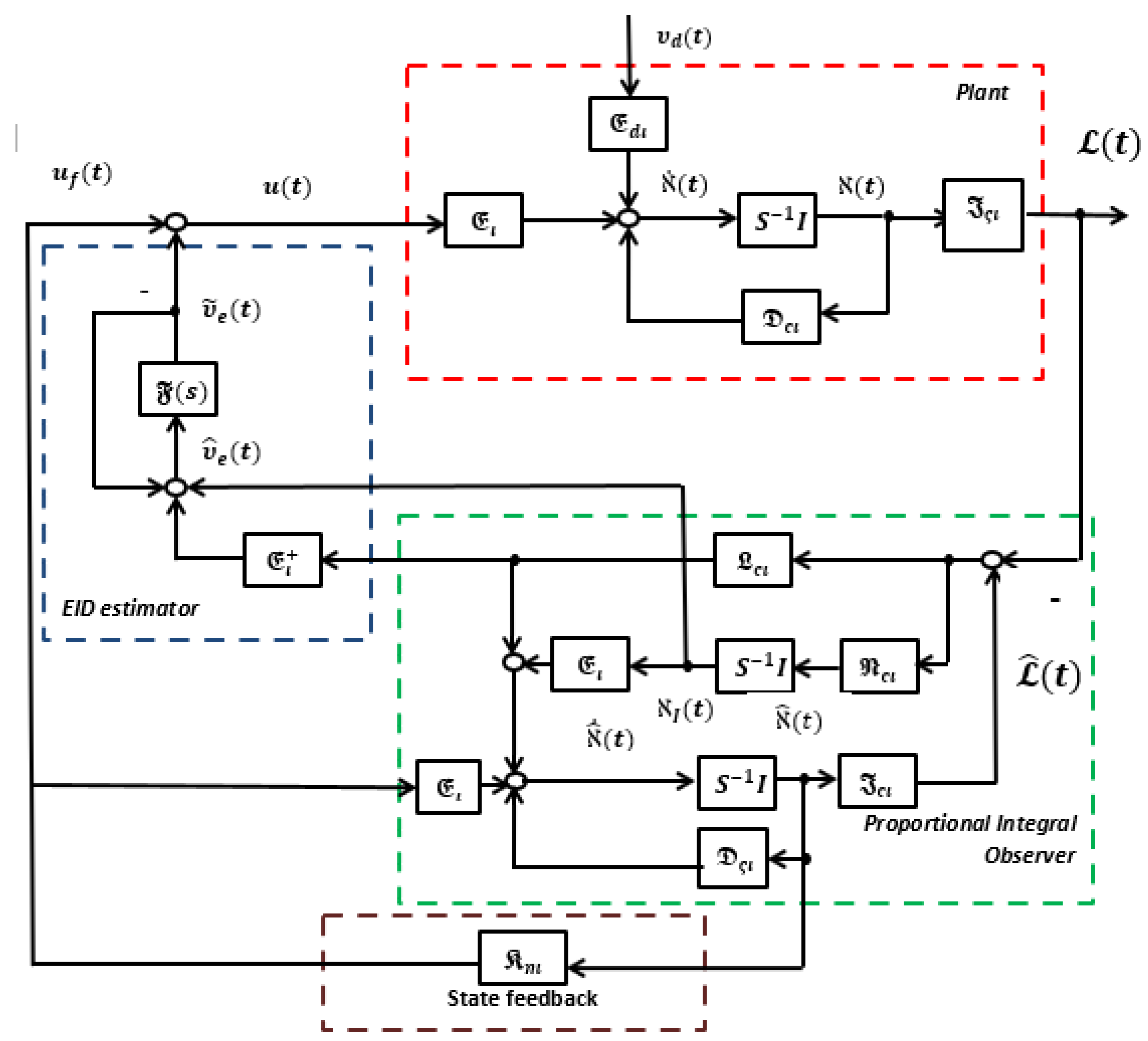
In Figure 1, the setup of an EID based control system with a PIO is depicted. It includes the plant, a state-feedback controller, a PIO, and an EID estimator. EID, as defined in [26], is a signal on the control input channel that affects the output in a manner similar to genuine disturbances. To start, we characterize the plant (2) using an EID ${\upsilon }_e\left(t\right)$. This gives:

$$\begin{array}{c}\hfill \left\{\begin{array}{c}\dot{\aleph }\left(t\right)={\displaystyle \sum _{\varsigma =1}^r}{\Im }_{\varsigma }(\ell \left(t\right))\left[{\mathfrak{D}}_{\varsigma \iota }\aleph \left(t\right)+{\mathfrak{E}}_{\iota }\left(u\left(t\right)+{\upsilon }_e\left(t\right)\right)\right],\hfill \\ \pounds \left(t\right)={\displaystyle \sum _{\varsigma =1}^r}{\Im }_{\varsigma }(\ell \left(t\right)){\mathfrak{J}}_{\varsigma \iota }\aleph \left(t\right),\hfill \end{array}\right.\end{array}$$

(4)

where the equivalent-input-disturbance ${\upsilon }_e\left(t\right)$ of ${\upsilon }_d\left(t\right)$ means that the output of the EID ${\upsilon }_e\left(t\right)$ is equal to the output produced by the real disturbance ${\upsilon }_d\left(t\right)$.

The PIO from [37] is utilized in this work to aid with system design. The PIO is represented in state space by:

$$\begin{array}{c}\hfill \left\{\begin{array}{c}\dot{\widehat{\aleph }}\left(t\right)={\displaystyle \sum _{\varsigma =1}^r}{\Im }_{\varsigma }(\ell \left(t\right))\left[{\mathfrak{D}}_{\varsigma \iota }\widehat{\aleph }\left(t\right)+{\mathfrak{E}}_{\iota }{u}_f\left(t\right)+{\mathfrak{L}}_{\varsigma \iota }[\pounds \left(t\right)-\widehat{\pounds }\left(t\right)]+{\mathfrak{E}}_{\iota }{\aleph }_I\left(t\right)\right],\hfill \\ \widehat{\pounds }\left(t\right)={\displaystyle \sum _{\varsigma =1}^r}{\Im }_{\varsigma }(\ell \left(t\right)){\mathfrak{J}}_{\varsigma \iota }\widehat{\aleph }\left(t\right),\hfill \\ {\dot{\aleph }}_I\left(t\right)={\displaystyle \sum _{\varsigma =1}^r}{\Im }_{\varsigma }(\ell \left(t\right)){\mathfrak{N}}_{\varsigma \iota }[\pounds \left(t\right)-\widehat{\pounds }\left(t\right)]-{\aleph }_I\left(t\right),\hfill \end{array}\right.\end{array}$$

(5)

where the estimated reconstructed states of $\aleph \left(t\right)$ and $\pounds \left(t\right)$ are indicated by $\widehat{\aleph }\left(t\right)\in {\mathbb{R}}^n$, $\widehat{\pounds }\left(t\right)\in {\mathbb{R}}^r$. $u_f\left(t\right)$ is the enhanced control input, and the proportional and integral gains, respectively, are ${\mathfrak{L}}_{\varsigma \iota }\in {\mathbb{R}}^{n\times r}$ and ${\mathfrak{N}}_{\varsigma \iota }\in {\mathbb{R}}^{r\times r}$. A vector named ${\aleph }_I\left(t\right)$ represents the integral of the weighted output estimation.

Remark 1.

In this study, it is assumed that the state variables in (4), which represents the measured output $\pounds \left(t\right)$, are unavailable. In order to estimate the measured output, the system in (4) is manually replicated with the same behavior to form the estimated output $\widehat{\pounds }\left(t\right)$ in (5). In particular, while replicating the actual system, a negligible error component $\Delta \pounds \left(t\right)=\pounds \left(t\right)-\widehat{\pounds }\left(t\right)$ is introduced. To be specific, when $t\to \infty$, $\Delta \pounds \left(t\right)\to 0$; thus, it is obvious that $\pounds \left(t\right)=\widehat{\pounds }\left(t\right)$. Hence, when $\widehat{\pounds }\left(t\right)$ converges to 0, $\pounds \left(t\right)$ will also converge to 0.

Further, the error dynamics between state (2) and the observer (5) are denoted by:

$$\begin{array}{c}\hfill \Delta \aleph \left(t\right)=\aleph \left(t\right)-\widehat{\aleph }\left(t\right),\end{array}$$

(6)

and substituting it to (4) yields:

$$\begin{array}{c}\hfill \left\{\begin{array}{c}\dot{\widehat{\aleph }}\left(t\right)={\displaystyle \sum _{\varsigma =1}^r}{\Im }_{\varsigma }(\ell \left(t\right))\left[{\mathfrak{D}}_{\varsigma \iota }\widehat{\aleph }\left(t\right)+{\mathfrak{E}}_{\iota }(u\left(t\right)+{\upsilon }_e\left(t\right))\right]+\left[{\mathfrak{D}}_{\varsigma \iota }\left(t\right)\Delta \aleph \left(t\right)-\Delta \dot{\aleph }\left(t\right)\right],\hfill \\ \widehat{\pounds }\left(t\right)={\displaystyle \sum _{\varsigma =1}^r}{\Im }_{\varsigma }(\ell \left(t\right)){\mathfrak{J}}_{\varsigma \iota }\widehat{\aleph }\left(t\right).\hfill \end{array}\right.\end{array}$$

(7)

If we add a control input $\Delta \upsilon \left(t\right)$, such that:

$$\begin{array}{c}\hfill {\mathfrak{E}}_{\iota }\Delta \upsilon \left(t\right)={\mathfrak{D}}_{\varsigma \iota }\left(t\right)\Delta \aleph \left(t\right)-\Delta \dot{\aleph }\left(t\right),\end{array}$$

(8)

then substituting (8) into (7) and allowing the estimated EID ${\upsilon }_e\left(t\right)$ to be:

$$\begin{array}{c}\hfill {\widehat{\upsilon }}_e\left(t\right)={\upsilon }_e\left(t\right)+\Delta \upsilon \left(t\right)\end{array}$$

(9)

allows us to denote the plant as:

$$\begin{array}{c}\hfill \left\{\begin{array}{c}\dot{\widehat{\aleph }}\left(t\right)={\displaystyle \sum _{\varsigma =1}^r}{\Im }_{\varsigma }(\ell \left(t\right))\left[{\mathfrak{D}}_{\varsigma \iota }\widehat{\aleph }\left(t\right)+{\mathfrak{E}}_{\iota }(u\left(t\right)+{\widehat{\upsilon }}_e\left(t\right))\right],\hfill \\ \pounds \left(t\right)={\displaystyle \sum _{\varsigma =1}^r}{\Im }_{\varsigma }(\ell \left(t\right)){\mathfrak{J}}_{\varsigma \iota }\aleph \left(t\right).\hfill \end{array}\right.\end{array}$$

(10)

It should be noticed that the FSMJSs (4) may contain disturbances, which may lead to the poor performance or instability of the system. Moreover, the EID approach does not need prior information about the disturbances, and it may efficiently estimate and reject both matched and unmatched disturbances. In this FSMJSs, an EID technique is employed in the control channel, which yields satisfactory disturbance rejection performance. The optimal EID estimated disturbance can be expressed by:

$$\begin{array}{c}\hfill {\widehat{\upsilon }}_e\left(t\right)=\sum _{\varsigma =1}^r{\Im }_{\varsigma }(\ell \left(t\right))\left[{\mathfrak{E}}_{\iota }^{+}{\mathfrak{L}}_{\varsigma \iota }{\mathfrak{J}}_{\varsigma \iota }\Delta \aleph \left(t\right)+u_f\left(t\right)-u\left(t\right)+{\aleph }_I\left(t\right)\right],\end{array}$$

(11)

where ${\mathfrak{E}}_{\iota }^{+}$ is the pseudo inverse of ${\mathfrak{E}}_{\iota }$. It is commonly known that external disruptions typically have frequencies in the low-frequency range. Therefore, developing a method to determine the disturbance in a particular low-frequency band makes sense. The frequency range for the disturbance calculation is chosen using a low-pass filter, $\mathfrak{F}\left(s\right)$ to achieve this.

$$\begin{array}{c}\hfill \left|\mathfrak{F}\left(j\varpi \right)\right|\approx 1,\forall \varpi \in [0,{\varpi }_r].\end{array}$$

(12)

Here, ${\varpi }_r$ is the highest angular frequency required for the EID estimation. It should be noted that the estimated total disturbance may contain some measurement noise. To eliminate this noise from ${\widehat{\upsilon }}_e\left(t\right)$, the low-pass-filter $\mathfrak{F}\left(s\right)$ is integrated together with the state observer. Then, the state–space form of $\mathfrak{F}\left(s\right)$ is considered as:

$$\begin{array}{c}\hfill \left\{\begin{array}{cc}{\dot{\aleph }}_{\nu }\left(t\right)\hfill & ={\mathfrak{D}}_{\nu }{\aleph }_{\nu }\left(t\right)+{\mathfrak{E}}_{\nu }\left[{\mathfrak{E}}_{\iota }^{+}{\mathfrak{L}}_{\varsigma \iota }{\mathfrak{J}}_{\varsigma \iota }\Delta \aleph \left(t\right)+u_f\left(t\right)-u\left(t\right)+{\aleph }_I\left(t\right)\right],\hfill \\ {\tilde{\upsilon }}_e\left(t\right)\hfill & ={\mathfrak{J}}_{\nu }{\aleph }_{\nu }\left(t\right)\hfill \end{array}\right.\end{array}$$

(13)

where the state of $\mathfrak{F}\left(s\right)$ is represented by ${\aleph }_{\nu }\left(t\right)$. The predicted noise signal is shown as ${\tilde{\upsilon }}_e\left(t\right)$. ${\mathfrak{D}}_{\nu },{\mathfrak{E}}_{\nu }$, and ${\mathfrak{J}}_{\nu }$ are constant parameters.

Remark 2.

It should be noted that the abovementioned conditions of the EID are used to construct an EID estimator, which estimates and rejects the unknown external disturbances. In particular, it shows the difference between the fuzzy state-observer error dynamics and its system parameters. This difference is also treated as the disturbance, since it is caused by modeling the error dynamics and unknown inputs. Further, it is added to the estimated disturbance and filtered by a first order low-pass filter. Finally, this disturbance is completely suppressed by the EID estimator. Therefore, the construction of this assumption is reasonable.

Remark 3.

It should be noticed that the PIO has an additional integrating term, $x_I\left(t\right)$, which raises the order of the state observer and enables quick and precise estimation of the system state. Additionally, the system flexibility is improved by an additional gain matrix ${\mathfrak{N}}_{\varsigma \iota }$ introduced in the PIO. The PIO combined with the EID offers stable and accurate disturbance rejection performance as well as a trustworthy disturbance estimate.

Next, we consider the stabilization problem of FSMJSs (2). In order to stabilize system (2), a fuzzy state feedback controller $u_f\left(t\right)$ of $\eta$-th rule is designed as follows.

Control rule $\eta$: If ${\Psi }_1\left(t\right)$ is ${{\rm Y}}_{\eta 1}$, ${\Psi }_2\left(t\right)$ is ${{\rm Y}}_{\eta 2}$, and ⋯${\Psi }_g\left(t\right)$ is ${{\rm Y}}_{\eta g}$, then:

$$\begin{array}{c}\hfill u_f\left(t\right)=\sum _{\eta =1}^r{\Im }_{\eta }(\ell \left(t\right)){\mathfrak{K}}_{\eta \iota }\widehat{\aleph }\left(t\right),\end{array}$$

(14)

where ${\mathfrak{K}}_{\eta \iota }\in {\mathbb{R}}^{m\times n}$ indicates the fuzzy controller gain. Eventually, the noise estimated disturbance ${\tilde{\upsilon }}_e\left(t\right)$ together with the state feedback control law $u_f\left(t\right)$ yields a new controller, which is given by

$$\begin{array}{c}\hfill u\left(t\right)=u_f\left(t\right)-{\tilde{\upsilon }}_e\left(t\right).\end{array}$$

(15)

Furthermore, the system internal stability condition does not depends on exogenous signals; hence, the exogenous signals ${\upsilon }_e\left(t\right)$ are assumed to be zero.

Remark 4.

The primary objective of this work is to stabilize the system (1); therefore, a state feedback control $u_f\left(t\right)$ is introduced in (14), which is a function of the estimated observer state $\widehat{\aleph }\left(t\right)$. The developed control law $u\left(t\right)$ in (15) is a combination of $u_f\left(t\right)$ and an EID estimator ${\tilde{\upsilon }}_e\left(t\right)$, which forces $\widehat{\aleph }\left(t\right)$ to zero for stabilizing the system. Therefore, the convergence of ℵ to zero implies the convergence of the measured output £ to zero from (1), and the developed controller significantly converges the estimate $\widehat{\aleph }$ to zero.

Moreover, the following equation is obtained when incorporating (15) in (13):

$$\begin{array}{cc}\hfill {\dot{\aleph }}_{\nu }\left(t\right)& ={\mathfrak{D}}_{\nu }{\aleph }_{\nu }\left(t\right)+{\mathfrak{E}}_{\nu }\left[{\mathfrak{E}}_{\iota }^{+}{\mathfrak{L}}_{\varsigma \iota }{\mathfrak{J}}_{\varsigma \iota }\Delta \aleph \left(t\right)+{\tilde{\upsilon }}_d\left(t\right)+{\aleph }_I\left(t\right)\right],\hfill \\ \hfill & =\left({\mathfrak{D}}_{\nu }+{\mathfrak{E}}_{\nu }{\mathfrak{J}}_{\nu }\right){\aleph }_{\nu }\left(t\right)+{\mathfrak{E}}_{\nu }{\mathfrak{E}}_{\iota }^{+}{\mathfrak{L}}_{\varsigma \iota }{\mathfrak{J}}_{\varsigma \iota }\Delta \aleph \left(t\right)+{\mathfrak{E}}_{\nu }{\aleph }_I\left(t\right).\hfill \end{array}$$

(16)

Furthermore, we define the error between the state (2) and observer (5) with the configuration $\Delta \aleph \left(t\right)=\aleph \left(t\right)-\widehat{\aleph }\left(t\right)$. Then, the corresponding error system can be written as:

$$\begin{array}{c}\hfill \left\{\begin{array}{cc}\Delta \dot{\aleph }\left(t\right)\hfill & ={\displaystyle \sum _{\varsigma =1}^r}{\Im }_{\varsigma }(\ell \left(t\right))\left[\left({\mathfrak{D}}_{\varsigma \iota }-{\mathfrak{L}}_{\varsigma \iota }{\mathfrak{J}}_{\varsigma \iota }\right)\Delta \aleph \left(t\right)+{\mathfrak{E}}_{\iota }\left({\upsilon }_d\left(t\right)-{\tilde{\upsilon }}_e\left(t\right)\right)-{\mathfrak{E}}_{\iota }{\aleph }_I\left(t\right)\right],\hfill \\ \Delta \pounds \left(t\right)\hfill & ={\displaystyle \sum _{\varsigma =1}^r}{\Im }_{\varsigma }(\ell \left(t\right)){\mathfrak{J}}_{\varsigma \iota }\Delta \aleph \left(t\right)\hfill \end{array}\right..\end{array}$$

(17)

For the sake of simplicity, we assume that the closed-loop system must satisfy the following stability requirement: ${\upsilon }_d\left(t\right)=0$.

$$\begin{array}{c}\hfill \left\{\begin{array}{cc}\Delta \dot{\aleph }\left(t\right)\hfill & ={\displaystyle \sum _{\varsigma =1}^r}{\Im }_{\varsigma }(\ell \left(t\right))\left[\left({\mathfrak{D}}_{\varsigma \iota }-{\mathfrak{L}}_{\varsigma \iota }{\mathfrak{J}}_{\varsigma \iota }\right)\Delta \aleph \left(t\right)-{\mathfrak{E}}_{\iota }{\mathfrak{J}}_{\nu }{\aleph }_{\nu }\left(t\right)-{\mathfrak{E}}_{\iota }{\aleph }_I\left(t\right)\right],\hfill \\ \Delta \pounds \left(t\right)\hfill & ={\displaystyle \sum _{\varsigma =1}^r}{\Im }_{\varsigma }(\ell \left(t\right)){\mathfrak{J}}_{\varsigma \iota }\Delta \aleph \left(t\right)\hfill \end{array}\right..\end{array}$$

(18)

The enhanced closed loop system resulting from the aforementioned equations with state vector $\phi \left(t\right)={\left[\begin{array}{cccc}{\widehat{\aleph }}^T\left(t\right)& \Delta {\aleph }^T\left(t\right)& {\aleph }_I^T\left(t\right)& {\aleph }_{\nu }^T\left(t\right)\end{array}\right]}^T$ can be defined as:

$$\begin{array}{cc}\hfill \dot{\phi }\left(t\right)& =\sum _{\varsigma =1}^r\sum _{\eta =1}^r{\Im }_{\varsigma }(\ell \left(t\right)){\Im }_{\eta }(\ell \left(t\right))\left[{\overline{\mathfrak{A}}}_{\varsigma \iota }\phi \left(t\right)\right],\hfill \end{array}$$

(19)

$$\begin{array}{cc}\hfill \overline{\pounds }\left(t\right)& =\sum _{\varsigma =1}^r{\Im }_{\varsigma }(\ell \left(t\right))\left[{\overline{\mathfrak{J}}}_{\varsigma \iota }\phi \left(t\right)\right],\hfill \end{array}$$

(20)

where

$$\begin{array}{cc}\hfill {\overline{\mathfrak{A}}}_{\varsigma \iota }& =\left[\begin{array}{cccc}{\mathfrak{D}}_{\varsigma \iota }+{\mathfrak{E}}_{\iota }{\mathfrak{K}}_{\eta \iota }& {\mathfrak{L}}_{\varsigma \iota }{\mathfrak{J}}_{\varsigma \iota }& {\mathfrak{E}}_{\iota }& 0\\ 0& {\mathfrak{D}}_{\varsigma \iota }-{\mathfrak{L}}_{\varsigma \iota }{\mathfrak{J}}_{\varsigma \iota }& -{\mathfrak{E}}_{\iota }& -{\mathfrak{E}}_{\iota }{\mathfrak{J}}_{\nu }\\ 0& {\mathfrak{N}}_{\varsigma \iota }{\mathfrak{J}}_{\varsigma \iota }& -I& 0\\ 0& {\mathfrak{E}}_{\nu }{\mathfrak{E}}_{\iota }^{+}{\mathfrak{L}}_{\varsigma \iota }{\mathfrak{J}}_{\varsigma \iota }& {\mathfrak{E}}_{\nu }& {\mathfrak{D}}_{\nu }+{\mathfrak{E}}_{\nu }{\mathfrak{J}}_{\nu }\end{array}\right],{\overline{\mathfrak{J}}}_{\varsigma \iota }=\left[\begin{array}{cccc}{\mathfrak{J}}_{\varsigma \iota }& 0& 0& 0\\ 0& {\mathfrak{J}}_{\varsigma \iota }& 0& 0\\ 0& 0& 0& 0\\ 0& 0& 0& 0\end{array}\right],\hfill \end{array}$$

and $\overline{\pounds }\left(t\right)={\left[\begin{array}{cccc}{\widehat{\pounds }}^T\left(t\right)& \Delta {\pounds }^T\left(t\right)& 0& 0\end{array}\right]}^T$ is the output of the augmented closed loop system (19).

Remark 5.

It is noted that the augmented system φ in (19) combines the vectors $\widehat{\aleph }\left(t\right)$ and $\Delta \aleph \left(t\right)$ but does have the term $\aleph \left(t\right)$. In addition, from (14) and (15), φ converges to zero. It is obvious that the terms $\widehat{\aleph }\left(t\right)$ and $\Delta \aleph \left(t\right)$ of the error dynamics in (6) converge to zero, achieving the convergence of $\aleph \left(t\right)$ to zero.

3. Main Results

The issue of the stabilization and disturbance rejection for FSMJSs based on the EID control via the PIO method is covered in this section. It is possible to create a new set of necessary conditions based on the LMI that ensure the closed-loop system (19) is stochastically stable by building a correct Lyapunov–Krasovskii functional (LKF).

Theorem 1.

For fixed positive scalars ${\vartheta }_1,{\vartheta }_2,$ and ${\vartheta }_3$, the closed-loop system (19) is stochastically stable, if there exist symmetric positive definite matrices ${\mathfrak{P}}_{\iota },{\mathfrak{Q}}_{\iota },{\mathfrak{R}}_{\iota },$ and $\mathfrak{S}$, such that the following inequalities are satisfied:

$$\begin{array}{c}\hfill \Pi =\left\{\begin{array}{c}\left[\begin{array}{cccc}{\left[{\Phi }_{\iota }^{\varsigma \varsigma }\right]}_{4\times 4}& {\Omega }_1& {\Omega }_3& {\Omega }_5\\ \ast & -{\Omega }_2& 0& 0\\ \ast & \ast & -{\Omega }_4& 0\\ \ast & \ast & \ast & -{\Omega }_6\end{array}\right]<0,(\varsigma =\eta ),\hfill \\ \left[\begin{array}{cccc}{\left[{\Phi }_{\iota }^{\varsigma \eta }+{\Phi }_{\iota }^{\eta \varsigma }\right]}_{4\times 4}& {\Omega }_1& {\Omega }_3& {\Omega }_5\\ \ast & -{\Omega }_2& 0& 0\\ \ast & \ast & -{\Omega }_4& 0\\ \ast & \ast & \ast & -{\Omega }_6\end{array}\right]<0,(\varsigma \ne \eta ),\hfill \end{array}\right.\end{array}$$

(21)

where the elements of Π are:

${\Phi }_{\iota 1,1}^{\varsigma \eta }=\mathrm{Sym}\{\frac{1}{{\vartheta }_1}{\mathfrak{P}}_{\iota }{\mathfrak{D}}_{\varsigma \iota }+\frac{1}{{\vartheta }_1}{\mathfrak{P}}_{\iota }{\mathfrak{E}}_{\iota }{\mathfrak{K}}_{\eta \iota }\}+{\epsilon }_{\iota \iota }\left(\mathfrak{l}\right)\frac{1}{{\vartheta }_1}{\mathfrak{P}}_{\iota }$, ${\Phi }_{\iota 1,2}^{\varsigma \eta }=\frac{1}{{\vartheta }_1}{\mathfrak{P}}_{\iota }{\mathfrak{L}}_{\varsigma \iota }{\mathfrak{J}}_{\varsigma \iota }$, ${\Phi }_{\iota 1,3}^{\varsigma \eta }=\frac{1}{{\vartheta }_1}{\mathfrak{P}}_{\iota }{\mathfrak{E}}_{\iota }$,

${\Phi }_{\iota 2,2}^{\varsigma \eta }=\mathrm{Sym}\{\frac{1}{{\vartheta }_2}{\mathfrak{Q}}_{\iota }{\mathfrak{D}}_{\varsigma \iota }-\frac{1}{{\vartheta }_2}{\mathfrak{Q}}_{\iota }{\mathfrak{L}}_{\varsigma \iota }{\mathfrak{J}}_{\varsigma \iota }\}+{\epsilon }_{\iota \iota }\left(\mathfrak{l}\right)\frac{1}{{\vartheta }_2}{\mathfrak{Q}}_{\iota }$, ${\Phi }_{\iota 2,3}^{\varsigma \eta }=-\frac{1}{{\vartheta }_2}{\mathfrak{Q}}_{\iota }{\mathfrak{E}}_{\iota }+{\mathfrak{J}}_{\varsigma \iota }^T{\mathfrak{N}}_{\varsigma \iota }^T\frac{1}{{\vartheta }_3}{\mathfrak{R}}_{\iota }$,

${\Phi }_{\iota 2,4}^{\varsigma \eta }=-\frac{1}{{\vartheta }_2}{\mathfrak{Q}}_{\iota }{\mathfrak{E}}_{\iota }{\mathfrak{J}}_{\nu }+{\left({\mathfrak{E}}_{\nu }{\mathfrak{E}}_{\iota }^{+}{\mathfrak{L}}_{\varsigma \iota }{\mathfrak{J}}_{\varsigma \iota }\right)}^T\mathfrak{S}$, ${\Phi }_{\iota 3,3}^{\varsigma \eta }=\mathrm{Sym}\{-\frac{1}{{\vartheta }_3}{\mathfrak{R}}_{\iota }\}+{\epsilon }_{\iota \iota }\left(\mathfrak{l}\right)\frac{1}{{\vartheta }_3}{\mathfrak{R}}_{\iota }$, ${\Phi }_{\iota 3,4}^{\varsigma \eta }={\mathfrak{E}}_{\nu }^T\mathfrak{S}$,

${\Phi }_{\iota 4,4}^{\varsigma \eta }=\mathrm{Sym}\{\mathfrak{S}{\mathfrak{D}}_{\nu }+\mathfrak{S}{\mathfrak{E}}_{\nu }{\mathfrak{J}}_{\nu }\}$,

${\Omega }_1=\frac{1}{{\vartheta }_1}\left[\sqrt{{\epsilon }_{\iota 1}}{\mathfrak{P}}_1^T,\dots ,\sqrt{{\epsilon }_{\iota (\iota -1)}}{\mathfrak{P}}_{(\iota -1)}^T,\sqrt{{\epsilon }_{\iota (\iota +1)}}{\mathfrak{P}}_{(\iota +1)}^T,\dots ,\sqrt{{\epsilon }_{\iota \mathfrak{T}}}{\mathfrak{P}}_{\mathfrak{T}}^T\right]$,

${\Omega }_3=\frac{1}{{\vartheta }_2}\left[\sqrt{{\epsilon }_{\iota 1}}{\mathfrak{Q}}_1^T,\dots ,\sqrt{{\epsilon }_{\iota (\iota -1)}}{\mathfrak{Q}}_{(\iota -1)}^T,\sqrt{{\epsilon }_{\iota (\iota +1)}}{\mathfrak{Q}}_{(\iota +1)}^T,\dots ,\sqrt{{\epsilon }_{\iota \mathfrak{T}}}{\mathfrak{Q}}_{\mathfrak{T}}^T\right]$,

${\Omega }_5=\frac{1}{{\vartheta }_3}\left[\sqrt{{\epsilon }_{\iota 1}}{\mathfrak{R}}_1^T,\dots ,\sqrt{{\epsilon }_{\iota (\iota -1)}}{\mathfrak{R}}_{(\iota -1)}^T,\sqrt{{\epsilon }_{\iota (\iota +1)}}{\mathfrak{R}}_{(\iota +1)}^T,\dots ,\sqrt{{\epsilon }_{\iota \mathfrak{T}}}{\mathfrak{R}}_{\mathfrak{T}}^T\right]$,

${\Omega }_2=\mathrm{diag}\{\frac{1}{{\vartheta }_1}{\mathfrak{P}}_1,\frac{1}{{\vartheta }_1}{\mathfrak{P}}_2,\dots ,\frac{1}{{\vartheta }_1}{\mathfrak{P}}_{\mathfrak{T}}\}$, ${\Omega }_4=\mathrm{diag}\{\frac{1}{{\vartheta }_2}{\mathfrak{Q}}_1,\frac{1}{{\vartheta }_2}{\mathfrak{Q}}_2,\dots ,\frac{1}{{\vartheta }_2}{\mathfrak{Q}}_{\mathfrak{T}}\}$,

${\Omega }_6=\mathrm{diag}\{\frac{1}{{\vartheta }_3}{\mathfrak{R}}_1,\frac{1}{{\vartheta }_3}{\mathfrak{R}}_2,\dots ,\frac{1}{{\vartheta }_3}{\mathfrak{R}}_{\mathfrak{T}}\}$.

Proof. 

Obtaining the stability criterion for the enhanced system (19) suffices to verify the stochastic stability for the considered FSMJSs (1). Let us build an LKF with the following structure for the enhanced system (19) for this purpose:

$$\begin{array}{c}\hfill \mathcal{V}(\phi \left(t\right),t,\iota )=\sum _{i=1}^4{\mathcal{V}}_i(\phi \left(t\right),t,\iota )={\phi }^T\left(t\right)\overline{{\mathfrak{W}}_{\iota }}\phi \left(t\right),\end{array}$$

(22)

where $\overline{{\mathfrak{W}}_{\iota }}=\mathrm{diag}\{\frac{1}{{\vartheta }_1}{\mathfrak{P}}_{\iota },\frac{1}{{\vartheta }_2}{\mathfrak{Q}}_{\iota },\frac{1}{{\vartheta }_3}{\mathfrak{R}}_{\iota },\mathfrak{S}\}$ are the positive definite matrices. By using the infinitesimal operator $\mathcal{L}\{.\}$ together with the solution of the augmented system (19) along with the mathematical expectation, we can have:

$$\begin{array}{cc}\hfill \mathcal{E}\left\{\mathcal{L}\mathcal{V}\right(\phi \left(t\right),t,\iota \left)\right\}& \le \mathcal{E}\{2{\phi }^T\left(t\right)\overline{{\mathfrak{W}}_{\iota }}\dot{\phi }\left(t\right)+{\phi }^T\left(t\right)\sum _{\wp =1}^{\mathfrak{T}}{\epsilon }_{\iota \wp }\overline{{\mathfrak{W}}_{\wp }}\phi \left(t\right)\}\hfill \\ \hfill & \le \mathcal{E}\{2\sum _{\varsigma =1}^r\sum _{\eta =1}^r{\Im }_{\varsigma }(\ell \left(t\right)){\Im }_{\eta }(\ell \left(t\right)){\phi }^T\left(t\right)\overline{{\mathfrak{W}}_{\iota }}{\overline{\mathfrak{A}}}_{\varsigma \iota }\phi \left(t\right)+{\phi }^T\left(t\right)\sum _{\wp =1}^{\mathfrak{T}}{\epsilon }_{\iota \wp }\overline{{\mathfrak{W}}_{\wp }}\phi \left(t\right)\}\hfill \end{array}$$

(23)

$$\begin{array}{cc}\hfill \mathcal{E}\left\{\mathcal{L}{\mathcal{V}}_1(\widehat{\aleph }\left(t\right),t,\iota )\right\}& =\mathcal{E}\{{\widehat{\aleph }}^T\left(t\right)\frac{1}{{\vartheta }_1}{\mathfrak{P}}_{\iota }\dot{\widehat{\aleph }}\left(t\right)+{\widehat{\aleph }}^T\left(t\right)\sum _{\wp =1}^{\mathfrak{T}}{\epsilon }_{\iota \wp }\frac{1}{{\vartheta }_1}{\mathfrak{P}}_{\wp }\widehat{\aleph }\left(t\right)\}\hfill \\ & =\mathcal{E}\{\sum _{\varsigma =1}^r\sum _{\eta =1}^r{\Im }_{\varsigma }(\ell \left(t\right)){\Im }_{\eta }(\ell \left(t\right)){\widehat{\aleph }}^T\left(t\right)\frac{1}{{\vartheta }_1}{\mathfrak{P}}_{\iota }\hfill \\ & \times \left[{\mathfrak{D}}_{\varsigma \iota }\widehat{\aleph }\left(t\right)+{\mathfrak{E}}_{\iota }{u}_f\left(t\right)+{\mathfrak{L}}_{\varsigma \iota }[\pounds \left(t\right)-\widehat{\pounds }\left(t\right)]+{\mathfrak{E}}_{\iota }{\aleph }_I\left(t\right)\right]\hfill \\ & +{\widehat{\aleph }}^T\left(t\right)\sum _{\wp =1}^{\mathfrak{T}}{\epsilon }_{\iota \wp }\frac{1}{{\vartheta }_1}{\mathfrak{P}}_{\wp }\widehat{\aleph }\left(t\right)\}\hfill \end{array}$$

(24)

$$\begin{array}{cc}\hfill \mathcal{E}\left\{\mathcal{L}{\mathcal{V}}_2(\Delta \aleph \left(t\right),t,\iota )\right\}& =\mathcal{E}\{\Delta {\aleph }^T\left(t\right)\frac{1}{{\vartheta }_2}{\mathfrak{Q}}_{\iota }\Delta \dot{\aleph }\left(t\right)+\Delta {\aleph }^T\left(t\right)\sum _{\wp =1}^{\mathfrak{T}}{\epsilon }_{\iota \wp }\frac{1}{{\vartheta }_2}{\mathfrak{Q}}_{\wp }\Delta \aleph \left(t\right)\}\hfill \\ \hfill & =\mathcal{E}\{\sum _{\varsigma =1}^r\sum _{\eta =1}^r{\Im }_{\varsigma }(\ell \left(t\right)){\Im }_{\eta }(\ell \left(t\right))\Delta {\aleph }^T\left(t\right)\frac{1}{{\vartheta }_2}{\mathfrak{Q}}_{\iota }\hfill \\ \hfill & \times \left[{\mathfrak{D}}_{\varsigma \iota }\Delta \aleph \left(t\right)-{\mathfrak{L}}_{\varsigma \iota }{\mathfrak{J}}_{\varsigma \iota }\Delta \aleph \left(t\right)-{\mathfrak{E}}_{\iota }{\aleph }_I\left(t\right)-{\mathfrak{E}}_{\iota }{\mathfrak{J}}_{\nu }{\aleph }_{\nu }\left(t\right)\right]\hfill \\ \hfill & +\Delta {\aleph }^T\left(t\right)\sum _{\wp =1}^{\mathfrak{T}}{\epsilon }_{\iota \wp }\frac{1}{{\vartheta }_2}{\mathfrak{Q}}_{\wp }\Delta \aleph \left(t\right)\}\hfill \end{array}$$

(25)

$$\begin{array}{cc}\hfill \mathcal{E}\left\{\mathcal{L}{\mathcal{V}}_3({\aleph }_I\left(t\right),t,\iota )\right\}& =\mathcal{E}\{{\aleph }_I^T\left(t\right)\frac{1}{{\vartheta }_3}{\mathfrak{R}}_{\iota }{\dot{\aleph }}_I\left(t\right)+{\aleph }_I^T\left(t\right)\sum _{\wp =1}^{\mathfrak{T}}{\epsilon }_{\iota \wp }\frac{1}{{\vartheta }_3}{\mathfrak{R}}_{\wp }{\aleph }_I\left(t\right)\}\hfill \\ \hfill & =\mathcal{E}\{\sum _{\varsigma =1}^r\sum _{\eta =1}^r{\Im }_{\varsigma }(\ell \left(t\right)){\Im }_{\eta }(\ell \left(t\right)){\aleph }_I^T\left(t\right)\frac{1}{{\vartheta }_3}{\mathfrak{R}}_{\iota }\left[{\mathfrak{N}}_{\varsigma \iota }{\mathfrak{J}}_{\varsigma \iota }\Delta \aleph \left(t\right)-{\aleph }_I\left(t\right)\right]\hfill \\ & +{\aleph }_I^T\left(t\right)\sum _{\wp =1}^{\mathfrak{T}}{\epsilon }_{\iota \wp }\frac{1}{{\vartheta }_3}{\mathfrak{R}}_{\wp }{\aleph }_I\left(t\right)\}\hfill \end{array}$$

(26)

$$\begin{array}{cc}\hfill \mathcal{E}\left\{\mathcal{L}{\mathcal{V}}_4({\aleph }_{\nu }\left(t\right),t,\iota )\right\}& =\mathcal{E}\left\{{\aleph }_{\nu }^T\left(t\right)\mathfrak{S}{\dot{\aleph }}_{\nu }\left(t\right)\right\}\hfill \\ \hfill & =\mathcal{E}\{\sum _{\varsigma =1}^r\sum _{\eta =1}^r{\Im }_{\varsigma }(\ell \left(t\right)){\Im }_{\eta }(\ell \left(t\right)){\aleph }_{\nu }^T\left(t\right)\hfill \\ \hfill & \times \mathfrak{S}\left[{\mathfrak{E}}_{\nu }{\mathfrak{E}}_{\iota }^{+}{\mathfrak{L}}_{\varsigma \iota }{\mathfrak{J}}_{\varsigma \iota }\Delta \aleph \left(t\right)+{\mathfrak{E}}_{\nu }{\aleph }_I\left(t\right)+({\mathfrak{D}}_{\nu }+{\mathfrak{E}}_{\nu }{\mathfrak{J}}_{\nu }){\aleph }_{\nu }\left(t\right)\right]\}.\hfill \end{array}$$

(27)

By applying the Schur complement lemma to the semi-Markovian terms in (24)–(26) and then combining Equations (24)–(27), we can obtain the LMI (21). Furthermore, it is obvious and simple to draw the conclusion that $\mathcal{E}\left\{\mathcal{L}\mathcal{V}\right(\phi \left(t\right),t,\iota \left)\right\}<0$, if the condition in (21) is true. In addition, the closed-loop system (19) is stochastically stable according to the Lyapunov stability theory and the aforementioned assessments. □

Theorem 2.

For fixed positive scalars ${\kappa }_1,{\vartheta }_1,{\vartheta }_2,$ and ${\vartheta }_3$, the closed-loop system (19) is stochastically stable, if there exist symmetric positive definite matrices, ${\mathfrak{X}}_{\iota },{\mathfrak{Y}}_{\iota },{\mathfrak{Z}}_{\iota },$ and $\mathfrak{M}$, and appropriate dimensional matrices, ${\mathfrak{V}}_{\eta \iota },{\mathfrak{U}}_{\varsigma \iota },$ and ${\mathfrak{H}}_{\varsigma \iota }$, such that the following inequalities are satisfied:

$$\begin{array}{c}\hfill \overline{\Pi }=\left\{\begin{array}{c}\left[\begin{array}{cccc}{\left[{\overline{\Phi }}_{\iota }^{\varsigma \varsigma }\right]}_{4\times 4}& {\overline{\Omega }}_1& {\overline{\Omega }}_3& {\overline{\Omega }}_5\\ \ast & -{\overline{\Omega }}_2& 0& 0\\ \ast & \ast & -{\overline{\Omega }}_4& 0\\ \ast & \ast & \ast & -{\overline{\Omega }}_6\end{array}\right]<0,(\varsigma =\eta ),\hfill \\ \left[\begin{array}{cccc}{\left[{\overline{\Phi }}_{\iota }^{\varsigma \eta }+{\overline{\Phi }}_{\iota }^{\eta \varsigma }\right]}_{4\times 4}& {\overline{\Omega }}_1& {\overline{\Omega }}_3& {\overline{\Omega }}_5\\ \ast & -{\overline{\Omega }}_2& 0& 0\\ \ast & \ast & -{\overline{\Omega }}_4& 0\\ \ast & \ast & \ast & -{\overline{\Omega }}_6\end{array}\right]<0,(\varsigma \ne \eta ),\hfill \end{array}\right.\end{array}$$

(28)

$$\begin{array}{c}\hfill \left[\begin{array}{cc}-{\kappa }_{1}I& {\mathfrak{Y}}_{\iota }{\mathfrak{J}}_{\varsigma \iota }^T-{\mathfrak{J}}_{\varsigma \iota }^T{\overline{\mathfrak{Y}}}_{\iota }^T\\ 0& -I\end{array}\right]<0,\end{array}$$

(29)

where the elements of $\overline{\Pi }$ are:

${\overline{\Phi }}_{\iota 1,1}^{\varsigma \eta }=\mathrm{Sym}\{{\mathfrak{D}}_{\varsigma \iota }{\vartheta }_1{\mathfrak{X}}_{\iota }+{\vartheta }_1{\mathfrak{E}}_{\iota }{\mathfrak{V}}_{\eta \iota }\}+{\epsilon }_{\iota \iota }\left(\mathfrak{l}\right){\vartheta }_1{\mathfrak{X}}_{\iota }$, ${\overline{\Phi }}_{\iota 1,2}^{\varsigma \eta }={\vartheta }_2{\mathfrak{U}}_{\varsigma \iota }{\mathfrak{J}}_{\varsigma \iota }$, ${\overline{\Phi }}_{\iota 1,3}^{\varsigma \eta }={\mathfrak{E}}_{\iota }{\vartheta }_3{\mathfrak{Z}}_{\iota }$,

${\overline{\Phi }}_{\iota 2,2}^{\varsigma \eta }=\mathrm{Sym}\{{\mathfrak{D}}_{\varsigma \iota }{\vartheta }_2{\mathfrak{Y}}_{\iota }-{\vartheta }_2{\mathfrak{U}}_{\varsigma \iota }{\mathfrak{J}}_{\varsigma \iota }\}+{\epsilon }_{\iota \iota }\left(\mathfrak{l}\right){\vartheta }_2{\mathfrak{Y}}_{\iota }$, ${\overline{\Phi }}_{\iota 2,3}=-{\mathfrak{E}}_{\iota }{\vartheta }_3{\mathfrak{Z}}_{\iota }+{\vartheta }_2{\mathfrak{H}}_{\varsigma \iota }{\mathfrak{J}}_{\varsigma \iota }^T$,

${\overline{\Phi }}_{\iota 2,4}^{\varsigma \eta }=-{\mathfrak{E}}_{\iota }{\mathfrak{J}}_{\nu }\mathfrak{M}+{\vartheta }_2{\mathfrak{J}}_{\varsigma \iota }^T{\mathfrak{U}}_{\varsigma \iota }^T{\mathfrak{E}}_{\nu }^T{\mathfrak{E}}_{\iota }^{+}$, ${\overline{\Phi }}_{\iota 3,3}^{\varsigma \eta }=\mathrm{Sym}\{-{\vartheta }_3{\mathfrak{Z}}_{\iota }\}+{\epsilon }_{\iota \iota }\left(\mathfrak{l}\right){\vartheta }_3{\mathfrak{Z}}_{\iota }$, ${\overline{\Phi }}_{\iota 3,4}^{\varsigma \eta }={\vartheta }_3{\mathfrak{Z}}_{\iota }{\mathfrak{E}}_{\nu }^T$,

${\overline{\Phi }}_{\iota 4,4}^{\varsigma \eta }=\mathrm{Sym}\{{\mathfrak{D}}_{\nu }\mathfrak{M}+{\mathfrak{E}}_{\nu }{\mathfrak{J}}_{\nu }\mathfrak{M}\}$,

${\overline{\Omega }}_1={\vartheta }_1\left[\sqrt{{\epsilon }_{\iota 1}}{\mathfrak{X}}_1^T,\dots ,\sqrt{{\epsilon }_{\iota (\iota -1)}}{\mathfrak{X}}_{(\iota -1)}^T,\sqrt{{\epsilon }_{\iota (\iota +1)}}{\mathfrak{X}}_{(\iota +1)}^T,\dots ,\sqrt{{\epsilon }_{\iota \mathfrak{T}}}{\mathfrak{X}}_{\mathfrak{T}}^T\right]$,

${\overline{\Omega }}_3={\vartheta }_2\left[\sqrt{{\epsilon }_{\iota 1}}{\mathfrak{Y}}_1^T,\dots ,\sqrt{{\epsilon }_{\iota (\iota -1)}}{\mathfrak{Y}}_{(\iota -1)}^T,\sqrt{{\epsilon }_{\iota (\iota +1)}}{\mathfrak{Y}}_{(\iota +1)}^T,\dots ,\sqrt{{\epsilon }_{\iota \mathfrak{T}}}{\mathfrak{Y}}_{\mathfrak{T}}^T\right]$,

${\overline{\Omega }}_5={\vartheta }_3\left[\sqrt{{\epsilon }_{\iota 1}}{\mathfrak{Z}}_1^T,\dots ,\sqrt{{\epsilon }_{\iota (\iota -1)}}{\mathfrak{Z}}_{(\iota -1)}^T,\sqrt{{\epsilon }_{\iota (\iota +1)}}{\mathfrak{Z}}_{(\iota +1)}^T,\dots ,\sqrt{{\epsilon }_{\iota \mathfrak{T}}}{\mathfrak{Z}}_{\mathfrak{T}}^T\right]$,

${\overline{\Omega }}_2=\mathrm{diag}\{{\vartheta }_1{\mathfrak{X}}_1,{\vartheta }_1{\mathfrak{X}}_2,\dots ,{\vartheta }_1{\mathfrak{X}}_{\mathfrak{T}}\}$, ${\overline{\Omega }}_4=\mathrm{diag}\{{\vartheta }_2{\mathfrak{Y}}_1,{\vartheta }_2{\mathfrak{Y}}_2,\dots ,{\vartheta }_2{\mathfrak{Y}}_{\mathfrak{T}}\}$,

${\overline{\Omega }}_6=\mathrm{diag}\{{\vartheta }_3{\mathfrak{Z}}_1,{\vartheta }_3{\mathfrak{Z}}_2,\dots ,{\vartheta }_3{\mathfrak{Z}}_{\mathfrak{T}}\}$.

Moreover, if the derived inequality (28) is feasible, then the stabilizing controller gain is given by ${\mathfrak{K}}_{\eta \iota }={\mathfrak{V}}_{\eta \iota }{\mathfrak{X}}_{\iota }^{-1}$, and the observer gains are given by ${\mathfrak{L}}_{\varsigma \iota }={\mathfrak{U}}_{\varsigma \iota }{\overline{\mathfrak{Y}}}_{\iota }^{-1}$ and ${\mathfrak{N}}_{\varsigma \iota }={\mathfrak{H}}_{\varsigma \iota }{\overline{\mathfrak{Y}}}_{\iota }^{-1}$.

Proof. 

It appears that inequality (21) has been transformed into an LMI-based constraint because it does not take the linear form. Let us define a few terms to that end: $\frac{1}{{\vartheta }_1}{\mathfrak{P}}_{\iota }^{-1}={\vartheta }_1{\mathfrak{X}}_{\iota }$, $\frac{1}{{\vartheta }_2}{\mathfrak{Q}}_{\iota }^{-1}={\vartheta }_2{\mathfrak{Y}}_{\iota }$, $\frac{1}{{\vartheta }_3}{\mathfrak{R}}_{\iota }^{-1}={\vartheta }_3{\mathfrak{Z}}_{\iota }$, and ${\mathfrak{S}}^{-1}=\mathfrak{M}$. Further, pre- and post-multiplying (21) by $\mathrm{diag}\left\{{\nu }_1{\mathfrak{X}}_{\iota },{\nu }_2{\mathfrak{Y}}_{\iota },{\nu }_3{\mathfrak{Z}}_{\iota },\mathfrak{M},I,I,I\right\}$, and setting up ${\mathfrak{V}}_{\eta \iota }={\mathfrak{K}}_{\eta \iota }{\mathfrak{X}}_{\iota }$, ${\mathfrak{U}}_{\varsigma \iota }={\mathfrak{L}}_{\varsigma \iota }{\overline{\mathfrak{Y}}}_{\iota }$, ${\mathfrak{H}}_{\varsigma \iota }={\mathfrak{N}}_{\varsigma \iota }{\overline{\mathfrak{Y}}}_{\iota }$, we can easily retrieve (28). Since it is not a linear equation, it is difficult to solve the equation ${\mathfrak{C}}_{\varsigma \iota }{\mathfrak{Y}}_{\iota }={\overline{\mathfrak{Y}}}_{\iota }{\mathfrak{C}}_{\varsigma \iota }$ using the MATLAB LMI toolbox. In order to circumvent the problem, the optimization strategy algorithm is taken into account for the assumptions ${\mathfrak{C}}_{\varsigma \iota }{\mathfrak{Y}}_{\iota }={\overline{\mathfrak{Y}}}_{\iota }{\mathfrak{C}}_{\varsigma \iota }$. It can thus be understood equivalently as ${\left[{\mathfrak{C}}_{\varsigma \iota }{\mathfrak{Y}}_{\iota }-{\overline{\mathfrak{Y}}}_{\iota }{\mathfrak{C}}_{\varsigma \iota }\right]}^T\left[{\mathfrak{C}}_{\varsigma \iota }{\mathfrak{Y}}_{\iota }-{\overline{\mathfrak{Y}}}_{\iota }{\mathfrak{C}}_{\varsigma \iota }\right]<{\kappa }_{1}I$, where ${\kappa }_1$ is a given positive scalar that is sufficiently small. Then, by using the Schur complement, the aforementioned inequality can be equivalently turned into (29). The closed-loop system (19) is stochastically stable, if the relations (28) and (29) are met.

As a result, the closed-loop system (19) meets the prerequisites for stochastic stability, which has been proved in Theorem 2. Since the TR matrix ${\epsilon }_{\iota \iota }\left(\mathfrak{l}\right)$ is time varying, it might be necessary to test an infinite number of LMIs to fulfill the criteria (28) in Theorem 2, which would be computationally inefficient. The next step is to create numerically feasible finite LMIs from the inequalities in (28). This problem is resolved by the subsequent theorem. □

Theorem 3.

For fixed positive scalars ${\kappa }_1,{\vartheta }_1,{\vartheta }_2,$ and ${\vartheta }_3$, the closed-loop system (19) is stochastically stable, if there exist symmetric positive definite matrices, ${\mathfrak{X}}_{\iota },{\mathfrak{Y}}_{\iota },{\mathfrak{Z}}_{\iota },$ and $\mathfrak{M}$, and appropriate dimensional matrices ${\mathfrak{V}}_{\eta \iota },{\mathfrak{U}}_{\varsigma \iota },$ and ${\mathfrak{H}}_{\varsigma \iota }$, such that the following inequalities are satisfied:

$$\begin{array}{c}\hfill {\overline{\Pi }}^{\left(j\right)}=\left\{\begin{array}{c}\left[\begin{array}{cccc}{\left[{\overline{\Phi }}_{\iota }^{\varsigma \varsigma \left(j\right)}\right]}_{4\times 4}& {\overline{\Omega }}_1^{\left(j\right)}& {\overline{\Omega }}_3^{\left(j\right)}& {\overline{\Omega }}_5^{\left(j\right)}\\ \ast & -{\overline{\Omega }}_2^{\left(j\right)}& 0& 0\\ \ast & \ast & -{\overline{\Omega }}_4^{\left(j\right)}& 0\\ \ast & \ast & \ast & -{\overline{\Omega }}_6^{\left(j\right)}\end{array}\right]<0,(\varsigma =\eta ),\hfill \\ \left[\begin{array}{cccc}{\left[{\overline{\Phi }}_{\iota }^{\varsigma \eta \left(j\right)}+{\overline{\Phi }}_{\iota }^{\eta \varsigma \left(j\right)}\right]}_{4\times 4}& {\overline{\Omega }}_1^{\left(j\right)}& {\overline{\Omega }}_3^{\left(j\right)}& {\overline{\Omega }}_5^{\left(j\right)}\\ \ast & -{\overline{\Omega }}_2^{\left(j\right)}& 0& 0\\ \ast & \ast & -{\overline{\Omega }}_4^{\left(j\right)}& 0\\ \ast & \ast & \ast & -{\overline{\Omega }}_6^{\left(j\right)}\end{array}\right]<0,(\varsigma \ne \eta ),\hfill \end{array}\right.\end{array}$$

(30)

where the elements of $\left[{\widehat{\Pi }}^{\left(j\right)}\right]$ are:

${\overline{\Phi }}_{\iota 1,1}^{\varsigma \eta \left(j\right)}=\mathrm{Sym}\{{\vartheta }_1{\mathfrak{D}}_{\varsigma \iota }{\mathfrak{X}}_{\iota }+{\vartheta }_1{\mathfrak{E}}_{\iota }{\mathfrak{V}}_{\eta \iota }\}+{\vartheta }_1{\epsilon }_{\iota \iota ,w}^{\left(j\right)}{\mathfrak{X}}_{\iota }$,

${\overline{\Phi }}_{\iota 2,2}^{\varsigma \eta \left(j\right)}=\mathrm{Sym}\{{\mathfrak{D}}_{\varsigma \iota }{\vartheta }_2{\mathfrak{Y}}_{\iota }-{\vartheta }_2{\mathfrak{U}}_{\varsigma \iota }{\mathfrak{J}}_{\varsigma \iota }\}+{\epsilon }_{\iota \iota ,w}^{\left(j\right)}{\vartheta }_2{\mathfrak{Y}}_{\iota }$, ${\overline{\Phi }}_{\iota 3,3}^{\varsigma \eta \left(j\right)}=\mathrm{Sym}\{-{\vartheta }_3{\mathfrak{Z}}_{\iota }\}+{\epsilon }_{\iota \iota ,w}^{\left(j\right)}{\vartheta }_3{\mathfrak{Z}}_{\iota }$,

${\overline{\Omega }}_1^{\left(j\right)}={\vartheta }_1\left[\sqrt{{\epsilon }_{\iota 1,w}^{\left(j\right)}}{\mathfrak{X}}_1^T,\dots ,\sqrt{{\epsilon }_{\iota (\iota -1),w}^{\left(j\right)}}{\mathfrak{X}}_{(\iota -1)}^T,\sqrt{{\epsilon }_{\iota (\iota +1),w}^{\left(j\right)}}{\mathfrak{X}}_{(\iota +1)}^T,\dots ,\sqrt{{\epsilon }_{\iota \mathfrak{T},w}^{\left(j\right)}}{\mathfrak{X}}_{\mathfrak{T}}^T\right]$,

${\overline{\Omega }}_3^{\left(j\right)}={\vartheta }_2\left[\sqrt{{\epsilon }_{\iota 1,w}^{\left(j\right)}}{\mathfrak{Y}}_1^T,\dots ,\sqrt{{\epsilon }_{\iota (\iota -1),w}^{\left(j\right)}}{\mathfrak{Y}}_{(\iota -1)}^T,\sqrt{{\epsilon }_{\iota (\iota +1),w}^{\left(j\right)}}{\mathfrak{Y}}_{(\iota +1)}^T,\dots ,\sqrt{{\epsilon }_{\iota \mathfrak{T},w}^{\left(j\right)}}{\mathfrak{Y}}_{\mathfrak{T}}^T\right]$,

${\overline{\Omega }}_5^{\left(j\right)}={\vartheta }_3\left[\sqrt{{\epsilon }_{\iota 1,w}^{\left(j\right)}}{\mathfrak{Z}}_1^T,\dots ,\sqrt{{\epsilon }_{\iota (\iota -1),w}^{\left(j\right)}}{\mathfrak{Z}}_{(\iota -1)}^T,\sqrt{{\epsilon }_{\iota (\iota +1),w}^{\left(j\right)}}{\mathfrak{Z}}_{(\iota +1)}^T,\dots ,\sqrt{{\epsilon }_{\iota \mathfrak{T},w}^{\left(j\right)}}{\mathfrak{Z}}_{\mathfrak{T}}^T\right]$,

${\overline{\Omega }}_2^{\left(j\right)}=\mathrm{diag}\{{\vartheta }_1{\mathfrak{X}}_1,{\vartheta }_1{\mathfrak{X}}_2,\dots ,{\vartheta }_1{\mathfrak{X}}_{\mathfrak{T}}\}$, ${\overline{\Omega }}_4^{\left(j\right)}=\mathrm{diag}\{{\vartheta }_2{\mathfrak{Y}}_1,{\vartheta }_2{\mathfrak{Y}}_2,\dots ,{\vartheta }_2{\mathfrak{Y}}_{\mathfrak{T}}\}$, and

${\overline{\Omega }}_6^{\left(j\right)}=\mathrm{diag}\{{\vartheta }_3{\mathfrak{Z}}_1,{\vartheta }_3{\mathfrak{Z}}_2,\dots ,{\vartheta }_3{\mathfrak{Z}}_{\mathfrak{T}}\}$, and the remaining parameters and inequalities are the same as in Theorem 2. For $j=1,2$, we have ${\epsilon }_{\iota \wp ,w}^{\left(1\right)}={\underline{\epsilon }}_{\iota \wp ,w}$ and ${\epsilon }_{\iota \wp ,w}^{\left(2\right)}={\overline{\epsilon }}_{\iota \wp ,w}$.

Proof. 

Theorem 2 makes it clear that assuming condition (28) holds, and the closed-loop system (19) accompanied by the time-varying TR matrix ${\epsilon }_{\iota \wp }\left(\mathfrak{l}\right)$ is robustly stochastically stable. The time-varying term ${\epsilon }_{\iota \wp }\left(\mathfrak{l}\right)$ is allowed to have a lower bound ${\underline{\epsilon }}_{\iota \wp }$ and an upper bound ${\overline{\epsilon }}_{\iota \wp }$ in order to ensure numerical tractability. There is no disagreement that this is a successful approach.

$$\begin{array}{c}\hfill {\underline{\epsilon }}_{\iota \wp }\le {\epsilon }_{\iota \wp }\left(\mathfrak{l}\right)\le {\overline{\epsilon }}_{\iota \wp }.\end{array}$$

(31)

As can be seen from (31), it is clear that ${\epsilon }_{\iota \wp }\left(\mathfrak{l}\right)$ takes any value in $\left[{\underline{\epsilon }}_{\iota \wp },{\overline{\epsilon }}_{\iota \wp }\right]$. In parallel, for a specific $\mathfrak{l}$, ${\epsilon }_{\iota \wp }\left(\mathfrak{l}\right)$ is a convex combination, as demonstrated below:

$$\begin{array}{c}\hfill {\epsilon }_{\iota \wp }\left(\mathfrak{l}\right)=\beta {\underline{\epsilon }}_{\iota \wp }+(1-\beta ){\overline{\epsilon }}_{\iota \wp },\end{array}$$

(32)

where $0\le \beta \le 1$, because ${\epsilon }_{\iota \wp }\left(\mathfrak{l}\right)$ in (32) is linearly dependent on $\beta$, and (28) only has to be satisfied for $\beta =0$ and $\beta =1$; that is, (28) holds if the inequalities in (30) hold. The proof of this theorem is also completed by splitting the sojourn time s into w pieces. □

4. Numerical Simulation

To demonstrate the theoretical viability of our strategy, we assume a system in this section that has two operating system modes and two fuzzy rules. The parameters are chosen in accordance with the following, and its model is identical to system (19):

${\mathfrak{D}}_{11}=\left[\begin{array}{cc}-2.9& -0.8\\ 1& -1.3\end{array}\right]$, ${\mathfrak{D}}_{21}=\left[\begin{array}{cc}-1.3& 0.5\\ -0.2& -2.4\end{array}\right]$, ${\mathfrak{D}}_{12}=\left[\begin{array}{cc}-2.8& -0.7\\ 0.8& -1.2\end{array}\right]$, ${\mathfrak{D}}_{22}=\left[\begin{array}{cc}-1.3& 0.5\\ -0.1& -2.1\end{array}\right]$,

${\mathfrak{E}}_{11}=\left[\begin{array}{c}0.5\\ -0.5\end{array}\right]$, ${\mathfrak{E}}_{21}=\left[\begin{array}{c}0.4\\ -0.8\end{array}\right]$, ${\mathfrak{E}}_{12}=\left[\begin{array}{c}0.2\\ -0.5\end{array}\right]$, ${\mathfrak{E}}_{22}=\left[\begin{array}{c}0.4\\ -0.7\end{array}\right]$, ${\mathfrak{J}}_{11}=\left[\begin{array}{cc}-0.7& 1.1\end{array}\right]$, ${\mathfrak{J}}_{21}=\left[\begin{array}{cc}-0.6& 0.9\end{array}\right]$, ${\mathfrak{J}}_{12}=\left[\begin{array}{cc}-0.6& 1.1\end{array}\right]$, ${\mathfrak{J}}_{22}=\left[\begin{array}{cc}-0.5& 0.9\end{array}\right]$, $\varsigma =1,2$, $\iota =1,2$.

We choose ${\aleph }_1\left({\aleph }_2\left(t\right)\right)=\frac{e^{-}\left({\aleph }_1-0.1\sin \left({\aleph }_1\right)-1\right)}{1+e^{-}\left({\aleph }_1-0.1\sin \left({\aleph }_1\right)-1\right)},{\aleph }_2\left({\aleph }_2\left(t\right)\right)=1-{\aleph }_1\left({\aleph }_2\left(t\right)\right)$ as the fuzzy membership function for simulation. The upper and lower bounded TR matrices are taken as $\underline{\epsilon }=\left[\begin{array}{cc}-1.8& 1.8\\ 1.1& -1.1\end{array}\right],\overline{\epsilon }=\left[\begin{array}{cc}-1.3& 1.3\\ 0.6& -0.6\end{array}\right]$. The other parameters are given as ${\kappa }_1={10}^{-4}$, ${\vartheta }_1=1$, ${\vartheta }_2=0.00001$, and ${\vartheta }_3=1$. A disturbance ${\upsilon }_e\left(t\right)=e^{-0.0001t}\sin \left(2t\right)$ is injected to the system. We select ${\varpi }_r$ to be $\pi$. The parameters of the low-pass filter $\mathfrak{F}\left(s\right)$ are chosen as ${\mathfrak{D}}_{\nu }=-101,{\mathfrak{E}}_{\nu }=100,$ and ${\mathfrak{J}}_{\nu }=1$, which satisfies (12). By utilizing the MATLAB LMI toolbox, a set of feasible solutions for Theorem 2 is discovered via LMIs (28) and (29), and the associated admissible gain matrices are started as ${\mathfrak{K}}_{11}=\left[1.42711.7615\right]$, ${\mathfrak{K}}_{21}=\left[1.41351.8423\right]$, ${\mathfrak{K}}_{12}=[-0.3380-0.9300]$, ${\mathfrak{K}}_{22}=[-0.3179-0.8896]$, ${\mathfrak{L}}_{11}=\left[\begin{array}{c}-0.8313\\ 0.3493\end{array}\right]$, ${\mathfrak{L}}_{21}=\left[\begin{array}{c}-0.8429\\ 0.3353\end{array}\right]$, ${\mathfrak{L}}_{12}=\left[\begin{array}{c}-0.9912\\ 1.7080\end{array}\right]$, ${\mathfrak{L}}_{22}=\left[\begin{array}{c}-0.7876\\ 1.7802\end{array}\right]$, ${\mathfrak{N}}_{11}=-0.0017$, ${\mathfrak{N}}_{21}=-0.0016$, ${\mathfrak{N}}_{12}=0.0028$, and ${\mathfrak{N}}_{22}=0.0036$. We plot the associated simulation graphs under the initial condition $\aleph \left(0\right)=\widehat{\aleph }\left(0\right)={[-23]}^T$, and ${\aleph }_I\left(0\right)=0.1$ and ${\aleph }_{\nu }\left(0\right)=0.1$, using the aforementioned gain matrices. 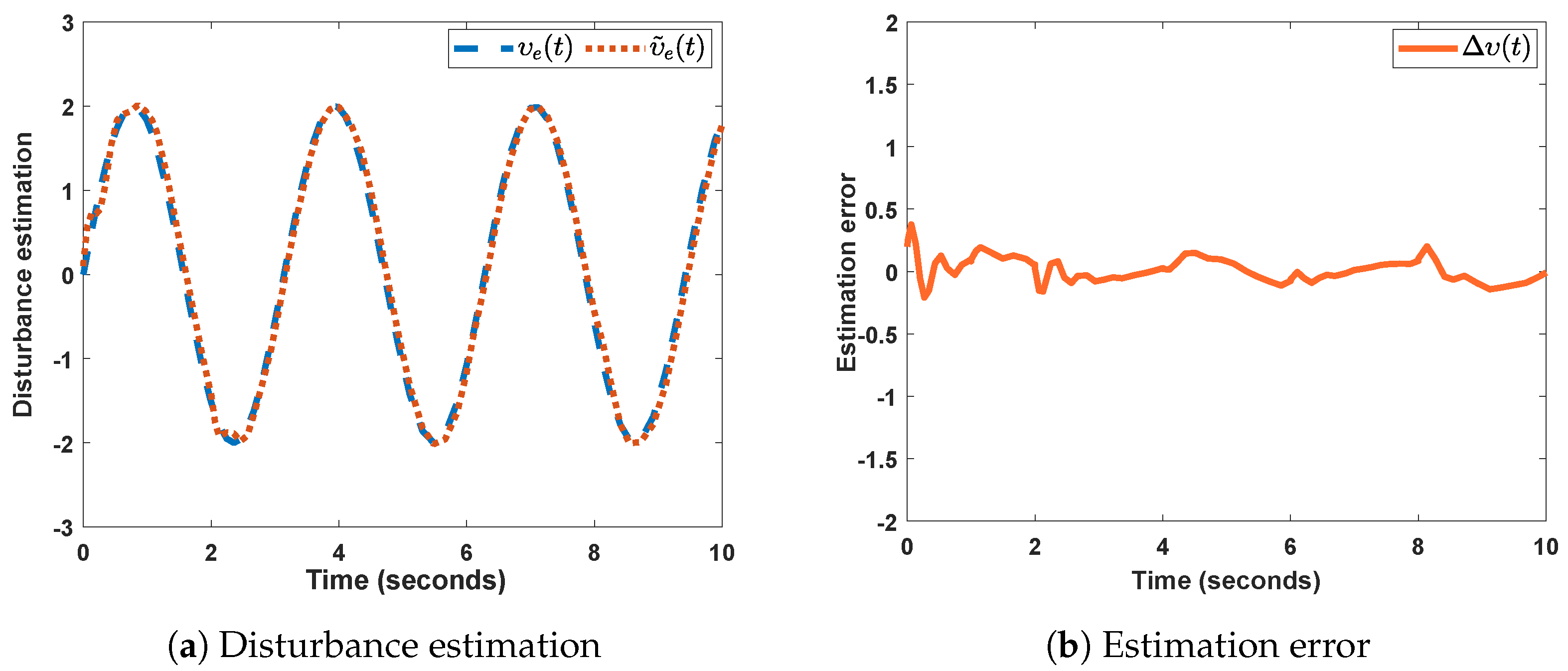The simulation results are shown in Figure 2, Figure 3, Figure 4, Figure 5, Figure 6, Figure 7, Figure 8, Figure 9 and Figure 10 employing the entire set of data described above. From Figure 2a, it is clear that the actual disturbance is completely estimated by the estimated disturbance, and its corresponding estimation error is displayed in Figure 2b. 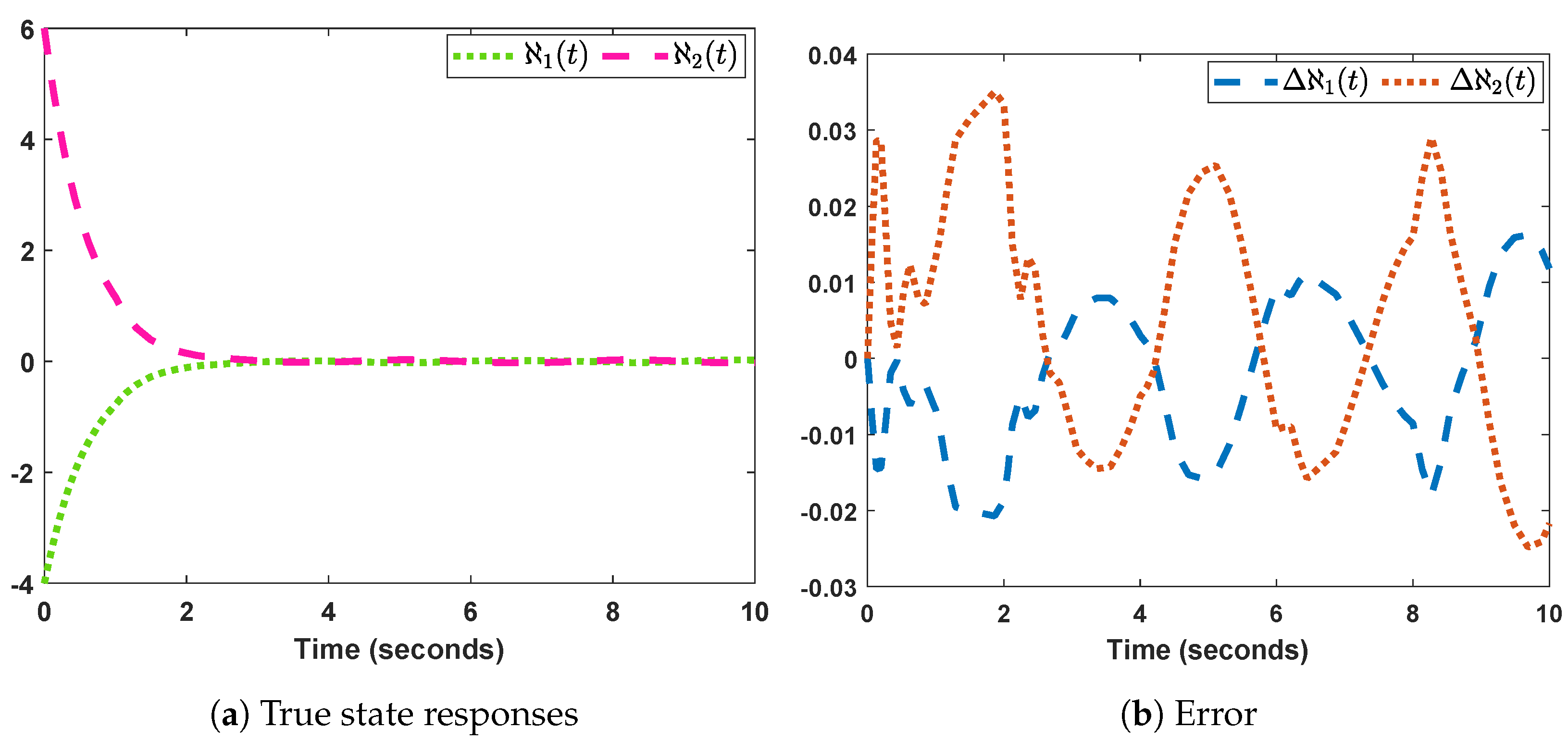Figure 3a,b shows, respectively, the system’s genuine state trajectory and associated error trajectory. 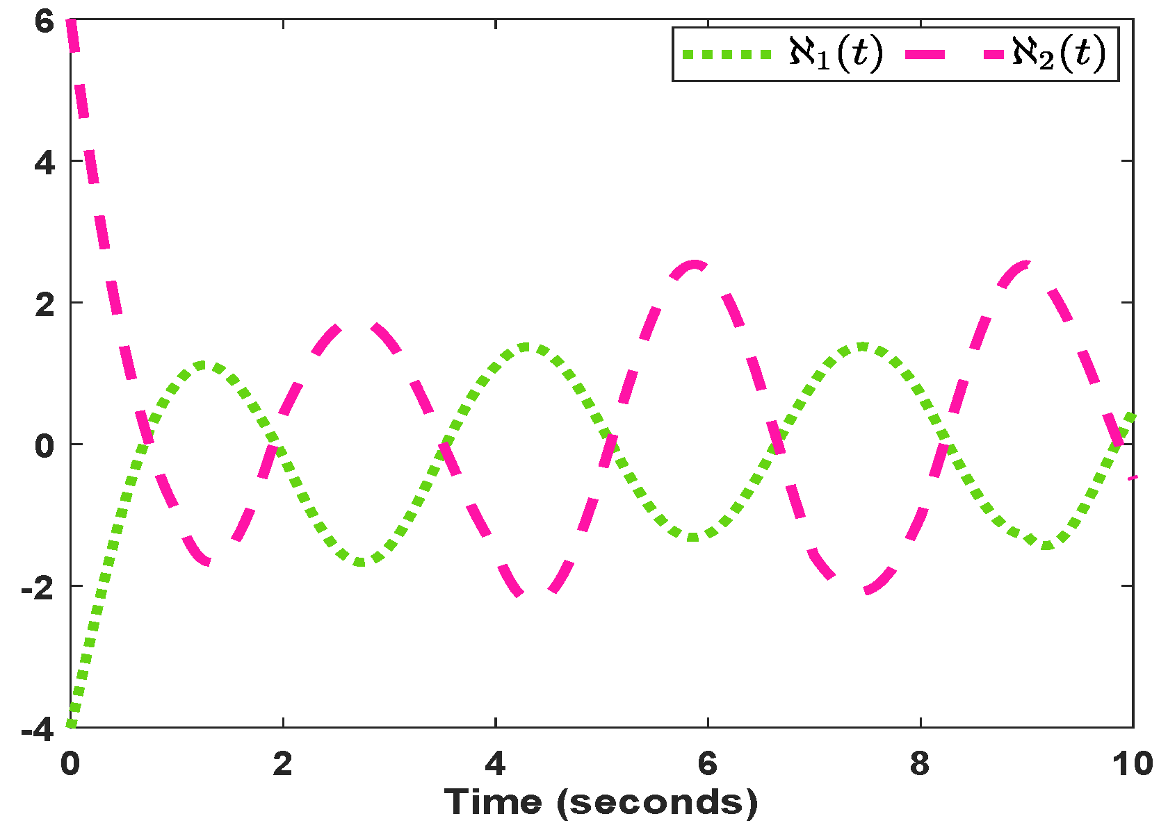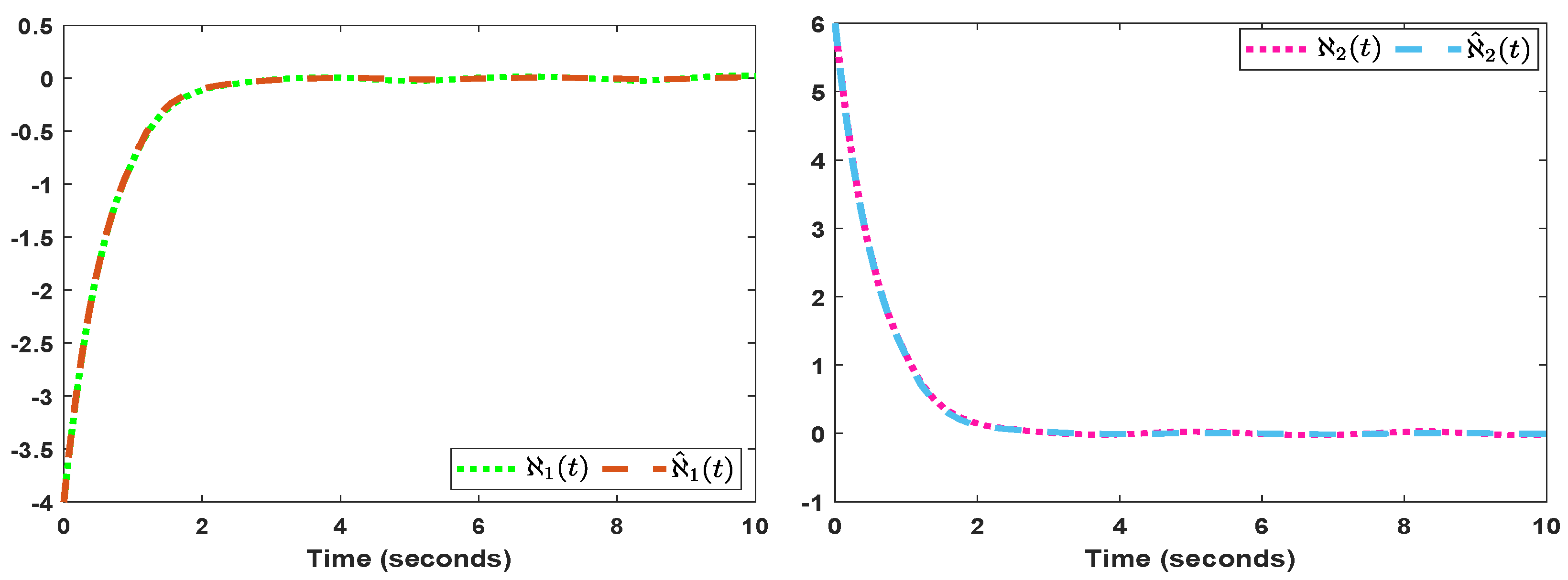Figure 4 shows the open-loop state trajectories. The state response curves of system along with its observer are presented in Figure 5a,b. 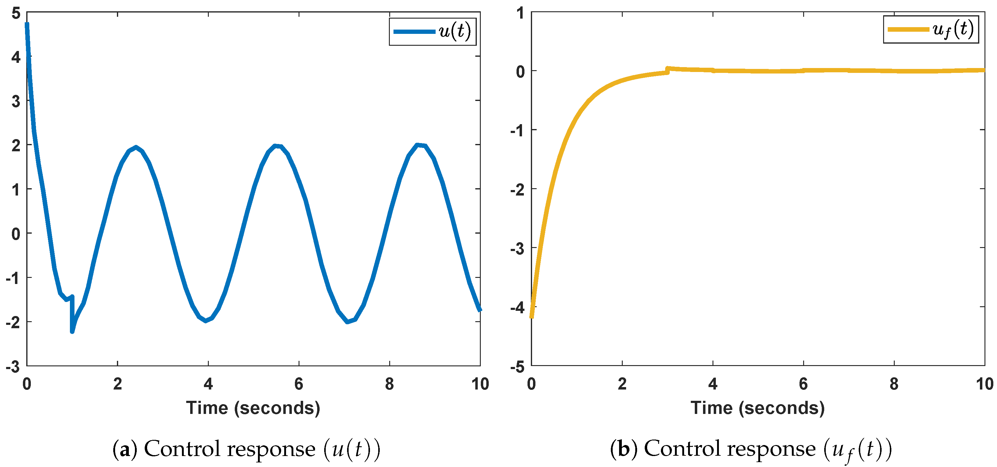Figure 6a displays the control responses. Furthermore, Figure 6b displays the control responses in the absence of a disturbance estimation ${\tilde{\upsilon }}_e\left(t\right)$. 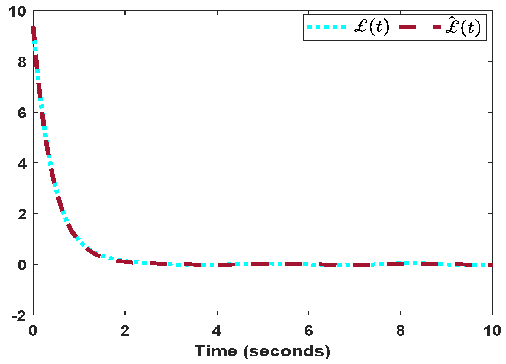The associated measured and observation output responses are displayed in Figure 7. 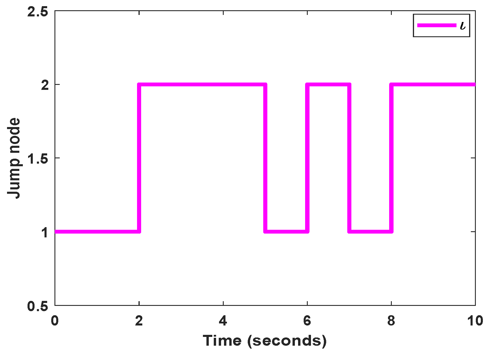In Figure 8, the membership functions are displayed. The jumping mode’s trajectory is also shown in Figure 9. 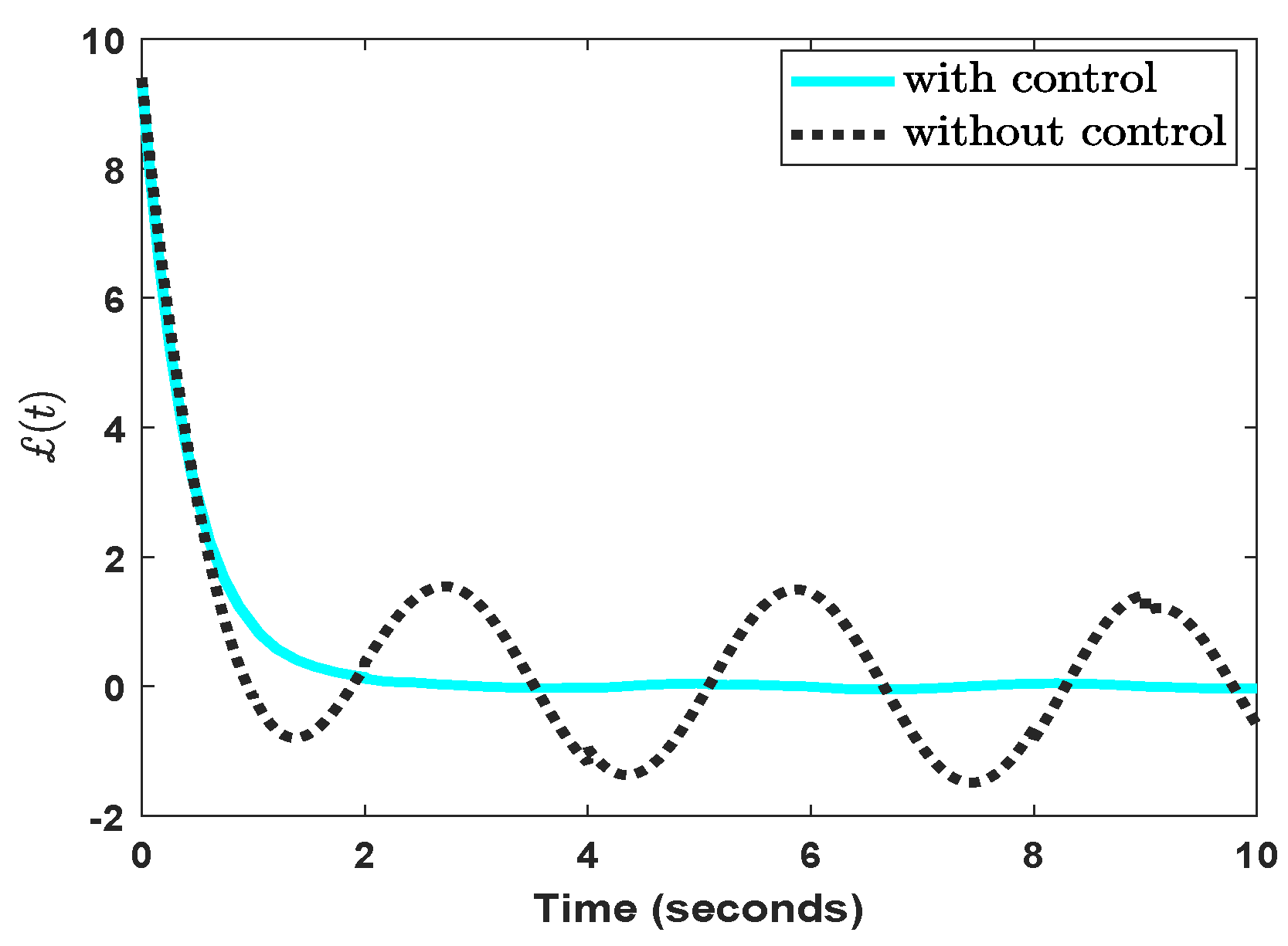Additionally, Figure 10 shows the outcomes of output response curves in the control absenteeism.

5. Conclusions

This work has examined FSMJSs in terms of the stability and disturbance rejection, utilizing the EID technique. A PIO was utilized in conjunction with an EID estimator to improve the accuracy of the state system estimation. LMIs were formulated to design the stability condition from the gain of the feedback controller and PIO. The simulation results showed that the proposed PIO-based EID technique achieved appropriate stability in addition to enhanced disturbance estimation and rejection capabilities. The intriguing subject of our future study will be how we may incorporate the PIO to further extend the suggested method for event-triggered fuzzy sliding-mode control with semi-Markovian switchings using EID for networked control systems.