Abstract
Regression analysis is a statistical process that utilizes two or more predictor variables to predict a response variable. When the predictors included in the regression model are strongly correlated with each other, the problem of multicollinearity arises in the model. Due to this problem, the model variance increases significantly, leading to inconsistent ordinary least-squares estimators that may lead to invalid inferences. There are numerous existing strategies used to solve the multicollinearity issue, and one of the most used methods is ridge regression. The aim of this work is to develop novel estimators for the ridge parameter “” and compare them with existing estimators via extensive Monte Carlo simulation and real data sets based on the mean squared error criterion. The study findings indicate that the proposed estimators outperform the existing estimators.
MSC:
62J05; 62J07; 62H20; 65C05
1. Introduction
Regression analysis predicts response variables using one or more predictor variables. In a variety of academic fields, including the social sciences, engineering, economics, and medicine, the predictor variables are highly intercorrelated. In such situations, the ordinary least-squares estimators (OLS) are inconsistent. Consequently, the OLS estimators have very large standard errors, and thus lead to wrong inferences. To overcome this issue, ref. [] introduced ridge regression, a technique that relies on biased estimation to reduce estimators’ overall variance. To control the trade-off between bias and variance, the ridge parameter , also known as the tuning parameter, is used.
To understand ridge regression, consider the following multiple linear regression equation:
where Y is an vector of the dependent variable, is a vector of unknown parameter, Z is an matrix of regression and is an vector of the error term, i.e.,
Generally, is considered to be independent and identically distributed, with mean 0 and variance , i.e.,
where is an identity matrix of order n, i.e.,
Furthermore, model (1) assumes that , , and , for .
The regression coefficient is unknown and must be estimated from the data. Usually, OLS estimators are used to estimate the regression coefficient by minimizing the sum of the squares of the residual, and the resulting OLS estimator is derived as
and
OLS estimators are typically preferred because they are the best linear unbiased estimator (BLUE), that is, they have the smallest variance among the set of unbiased estimators. However, their performance is heavily dependent on the matrix . If the matrix is ill-conditioned, i.e., if det , it indicates that there exists a multicollinearity problem. In other words, there exists at least a pair of regressors that are highly correlated (linearly dependent). In such cases, the OLS estimators are inconsistent and have large variance. In addition, some of the regression coefficients may be statistically insignificant or have the wrong sign, and thus can be misleading [].
One of the most effective approaches to address the issue of multicollinearity is ridge regression, which is suggested by many researchers. To address the issue of multicollinearity, ref. [] originally suggested ridge regression. To avoid overfitting, they added a small positive integer to the diagonal elements of the matrix via a penalty term in the loss function. The ridge regression estimator was then obtained mathematically by minimizing
This minimization leads to the ridge regression estimator
which is a biased estimator of , i.e.,
The estimator in Equation (4) is known as a ridge regression estimator, where plays an important role in the consistency of the estimator. When , , i.e., we obtain a stable but biased estimator of . On the other hand, when , OLS, and we obtain an unbiased but unstable estimator of . Furthermore, for a positive value of , this estimator provides a smaller mean-squared error (MSE) compared to the OLS [].
As plays an important role in the estimation of , ref. [] suggested that the value of should be small enough so that the MSE of the ridge estimator is less than the OLS. To this end, the researcher proposed different methods to estimate the value of , and the performance of the proposals was evaluated using simulation studies as well as real data sets. The MSE has generally been used as a performance criterion. As the ridge estimator is heavily dependent on the unknown value of , the optimum value for that can produce the best results is to some extent still an open problem in the literature. The estimator is a complicated function of , and several authors have presented their proposals for the estimation of [,,,,,,,,,,,,,,,,].
For example, ref. [] suggested an algorithm for choosing the tuning parameter in the ridge regression. The proposed algorithm has the following properties: it produces an average squared error for the regression coefficients that is less than the least-squares method; the estimate derived from the proposed method has a smaller variance than that of the least-squares method; and irrespective of the signal-to-noise ratio, the probability that the ridge produces a smaller squared error than the least-squares method is greater than 0.50. In addition, the simulation study shows that the proposed method performs better than the least-squares method. Ref. [] introduced a new method for selecting the ridge tuning parameter. The performance of the proposal was evaluated by simulation techniques using the MSE. Simulation results show that the MSE from their proposed method was smaller than using the Hoerl and Kennard ridge regression estimator.
Ref. [] suggested four modified versions of [] to select the ridge parameter () when multicollinearity exists in the design matrix columns. These estimators are compared to the [] using the MSE criterion. All estimators were tested using simulation criteria under certain conditions where a variety of variables that may influence their properties have been varied. It was shown that at least one of the proposed estimators either has a lower MSE than the others or is the next best.
Considering the generalized ridge regression approach, ref. [] proposed some new methods for estimating the ridge parameter . The proposed estimators, known as KAM, KGM, and KMed, were constructed using the arithmetic mean, geometric mean, and median of the [] estimator. Based on the MSE criterion, the simulation studies and real data results suggest the superiority of the proposed approach compared to some existing estimators. Based on different percentiles, ref. [] compared some new and old ridge regression estimators. The performance of the new estimators were evaluated using simulation studies and real data sets. It was observed that the proposed estimators are more efficient than the existing estimators.
Ref. [] presented a novel ridge estimator and compared it to well-established methods. Their estimator outperformed existing methods, according to the simulation studies and applications to real data sets. Furthermore, ref. [] introduced some new ridge estimators based on the Jackknife algorithm and compared their performance with existing ridge regression estimation using Monte Carlo simulations and real data sets. Their findings showed that the proposed estimators outperformed the competitors, and they concluded that ridge parameter estimates computed using Jackknife techniques are substantially better.
The main aim of this work was to propose efficient ridge estimators that are flexible and robust in the presence of multicollinearity. To this end, some of the existing estimators were modified, which resulted in three novel estimators of ridge parameters, which are NIS1, NIS2, and NIS3. To examine the performance of the proposals, different variables were varied throughout the simulation study, with errors being generated from two different probability distributions. Finally, the proposed estimators were tested using an extensive simulation study, as well as real datasets. The rest of the article is organized as follows. Section 2 introduces notations and preliminaries, followed by some existing and our proposed ridge estimators. Based on different variables, simulation settings are discussed in Section 3. A comprehensive simulation analysis is provided in Section 4. Section 5 assesses the performance of the proposed estimators on real datasets. Finally, Section 6 provides the conclusion of the study.
2. Existing and Proposed Ridge Estimators
This section presents the general ridge regression model in detail and proposes some new estimators for the ridge parameter . For this purpose, assume an orthogonal matrix D exists such that . The matrix is a diagonal matrix containing on its diagonal, which are the eigenvalues of the matrix C, where . Then, Equation (1) can be generalized as
where and . Consequently, the generalized ridge regression estimator can be obtained as
where and is the OLS estimates of .
2.1. Some Existing Estimators
Following on from the description of the basic ridge regression estimator, this section reviews some of previously developed ridge estimators for estimating the ridge parameter .
Hoerl and Kennard Estimator (1970)
Ref. [] suggested a ridge estimator by replacing and with their corresponding unbiased estimators, that is,
where is the residual mean square estimate, which is an unbiased estimator of ; and is the ith element of , which is an unbiased estimator of . Ref. [] offered an estimator for the ridge parameter based on the maximum value of , that is,
where the residual mean square error is an unbiased estimator of .
2.2. Kibria Estimator (2003)
Using the geometric mean of the vector , ref. [] offered a novel estimator based on the generalized ridge regression technique. The estimator is
A second estimator for the ridge parameter was also developed by [] by using the median of the estimator values in Equation (6), that is,
2.3. Khalaf, Mansson, and Shukar (2005)
A modified form of was proposed by [] for the estimation of ridge parameter , given as
Here, represents the maximum eigenvalue of the matrix .
2.4. Khalaf Alkhamisi Modified (2006)
Using the generalized ridge regression approach, ref. [] suggested a new estimator for estimating the ridge parameter , given as
2.5. Muniz and Kibria Estimator (2009)
Using the square root transformation of Equation (6), ref. [] proposed the following estimators for the estimation of the parameter :
where .
2.6. Proposed Estimators
For the ridge parameter, several estimators have been proposed by many researchers; however, none of them have consistently outperformed all other estimators. This has inspired us to reconsider the problem of estimating the ridge parameter and offer some new developments to the existing estimators that can perform well in a range of scenarios. In this study, some existing estimators are modified to propose some ridge parameters. In order to achieve this, the first proposed estimator is defined as
where CN refers to the condition number given as
where and are the maximum and minimum eigenvalues of the matrix . Our second proposed estimator is defined as
The third and final estimator we propose is:
Note that the proposed estimators are functions of the eigenvalues, the number of predictors, the standard deviation, and the number of observations. Thus, they contain a significant amount of information to determine an optimum value of the ridge parameter. In addition, they are highly flexible and robust to the varying values of different parameters.
3. Monte Carlo Simulation
The purpose of this section is to compare the performance of the existing ridge estimators to our suggested estimators. Specifically, it will evaluate the performance of the existing estimators HK, KGM, KMS, MKED, KSM, MK, and OLS and compare it to the performance of our proposed estimators NIS1, NIS2, and NIS3 based on the extensive Monte Carlo simulation.
3.1. Generating Predictor Variables
To conduct simulation studies, the initial step is to generate the explanatory variables and the response variable. To accomplish this, the explanatory variables were generated using the following equation:
where denotes the linear correlation between independent variables, are pseudo-random numbers generated from the standard normal distribution and Student-t distribution, and p denotes the number of explanatory variables. Once the predictors are generated, the response variable is determined as
where is an independent and identically distributed standard normal random variable with mean zero and variance , and n is the total number of observations.
3.2. Simulation Settings
The performance of an estimator can be affected by several factors, including sample size n, the correlation between independent variables , the number of independent variables p, and the error standard deviation . Therefore, in the simulation studies, we consider different values to evaluate the effect of these factors. In particular, we consider three different values for the correlation coefficient, i.e., = 0.90, 0.95, 0.99, sample size, n = 25, 50, 100, and the number of variables p = 4, 8, and 16. Furthermore, we consider the error terms with the following variances: = 1, 3, 5, 10, and 16. Furthermore, the explanatory variables are generated from two populations: normal and Student-t. Our main concern is the performance of the proposed estimators compared to the existing estimators. We consider high correlation values between independent variables, i.e., = 0.90, 0.95, and 0.99, to see how our proposed estimators perform in the presence of multicollinearity. In addition, we consider different sample sizes n = 25, 50, 100 to assess the effect of sample size. Moreover, the error terms are generated from the normal distribution as well as the Student-t distribution, considering a small, moderate, and large degree of freedom to see the effect of the distribution on the simulation studies.
3.3. Performance Evaluation Criteria
To evaluate the performance of the estimators, we used the MSE criterion, which can be mathematically expressed as
where is the estimator of obtained through the OLS or ridge estimator and N denotes the number of replications used in the Monte Carlo simulations. As the MSE balances the trade-off between bias and sampling variance, researchers extensively used this criterion to select an optimum value of the ridge parameter. To achieve a reliable estimate of , the simulation studies were repeated 2000 times, and thus, 2000 MSEs were computed, one each for every replication. Using the MSE, we compared our proposed estimator to the OLS and other existing ridge estimators described earlier. The results of the simulation studies are given in the following section.
4. Simulation Study Results
Throughout the simulation setting, a number of parameters were changed, including the standard deviation of the error term , the correlation coefficient , the sample size n, and the number of explanatory variables p, to test the effectiveness of the different estimators on simulated data sets. The results in Table 1, Table 2, Table 3, Table 4, Table 5, Table 6, Table 7, Table 8 and Table 9 refer to the scenario in which the pseudorandom numbers are generated from the standard normal distribution, and the results of the simulation data that are generated from Student-t distribution with various degrees of freedom are listed in Table 10, Table 11, Table 12, Table 13, Table 14, Table 15, Table 16, Table 17 and Table 18.

Table 1.
Estimated MSEs considering = 0.90, p = 4, and n = 25, 50, and 100 (superscript represents ranks).
Table 2.
Estimated MSEs considering = 0.95, p = 4, and n = 25, 50, and 100 (superscript represents ranks).
Table 3.
Estimated MSEs considering = 0.99, p = 4, and n = 25, 50, and 100 (superscript represents ranks).
Table 4.
Estimated MSEs considering = 0.90, p = 8, and n = 25, 50, and 100 (superscript represents ranks).
Table 5.
Estimated MSEs considering = 0.95, p = 8, and n = 25, 50, and 100 (superscript represents ranks).
Table 6.
Estimated MSEs considering = 0.99, p= 8, and n = 25, 50, and 100 (superscript represents ranks).
Table 7.
Estimated MSEs considering = 0.90, p = 16, and n = 25, 50, and 100 (superscript represents ranks).
Table 8.
Estimated MSEs considering = 0.95, p = 16, and n = 25, 50, and 100 (superscript represents ranks).
Table 9.
Estimated MSEs considering = 0.99, p = 16, and n = 25, 50, and 100 (superscript represents ranks).
Table 10.
Estimated MSEs considering = 0.90, p = 4, and n = 25, 50, and 100 (superscript represents ranks).
Table 11.
Estimated MSEs considering = 0.95, p = 4, and n = 25, 50, and 100 (superscript represents ranks).
Table 12.
Estimated MSEs considering = 0.99, p = 4, and n = 25, 50, and 100 (superscript represents ranks).
Table 13.
Estimated MSEs considering = 0.90, p = 8, and n = 25, 50, and 100 (superscript represents ranks).
Table 14.
Estimated MSEs considering = 0.95, p = 8, and n = 25, 50, and 100 (superscript represents ranks).
Table 15.
Estimated MSEs considering = 0.99, p = 8, and n = 25, 50, and 100 (superscript represents ranks).
Table 16.
Estimated MSEs considering = 0.90, p = 16, and n = 25, 50, and 100 (superscript represents ranks).
Table 17.
Estimated MSEs considering = 0.95, p = 16, and n = 25, 50, and 100 (superscript represents ranks).
Table 18.
Estimated MSEs considering = 0.99, p = 16, and n = 25, 50, and 100 (superscript represents ranks).
In general, the results shown in Table 1, Table 2, Table 3, Table 4, Table 5, Table 6, Table 7, Table 8, Table 9, Table 10, Table 11, Table 12, Table 13, Table 14, Table 15, Table 16, Table 17 and Table 18 show that the correlation coefficient and sample size n have a significant influence on the estimator’s MSE; as the degree of correlation increases, the MSE also increases for all estimators. Although the MSE value decreases with increasing sample size, it increases with increasing standard deviation of errors. Furthermore, our suggested estimators outperform other estimators as the degree of correlation increases. The probability distribution used in the data generation process has an impact on the results as well. In the following, we elaborate each table’s results separately.
Table 1 reports the results for different estimators used in the study, considering = 0.90, p = 4, n = 25, 50, 100, and = 1, 5, 10, and 16. From the results, it is evident that our proposed estimators outperformed the OLS and existing ridge estimators. Within our proposed estimators, the NIS2 produced the smallest MSE values compared to NIS1 and NIS3. The cumulative rank of NIS2 was 14, whereas NIS1 and NIS3 had ranks of 36 and 22, respectively. From the existing ridge estimators, the KGM performed relatively better than the other existing estimators used in the study by securing a cumulative rank of 48. Moreover, the effect of sample size on the MSE was significant; as the sample sizes increased, the overall MSEs decreased. On the other hand, when the residual standard error increased, the overall MSEs increased. Furthermore, the OLS performed poorly, as it produced the highest MSE in every situation, indicating that it cannot be used in a situation of high correlation among predictors.
Considering = 0.95, Table 2 reports the results for the proposed and existing ridge estimators for n= 25, 50, 100; p = 4; and = 1, 5, 10, and 16. By increasing the correlation value, the results indicate that the MSEs significantly increased for the OLS and the existing ridge, whereas it did not affect the size of the MSE of the proposed estimators. In addition, the proposed estimators outperformed the OLS and the existing estimators in every situation. Within our proposed estimators, the performance of NIS3 is evident, as it produced the smallest MSE values compared to NIS1 and NIS2. The cumulative rank of NIS3 was 17, whereas NIS1 and NIS2 had ranks of 36 and 19, respectively. On the other hand, the sample size positively affected MSE, as it decreased with the increase in sample size, whereas the residual standard error negatively affected MSE, i.e., a high value of produced a high value of the MSE. Again, the poor performance of the OLS is evident from the results in the case of high correlation among predictors.
The results listed in Table 3 correspond to = 0.99, whereas all other variables are the same as those used in Table 1 and Table 2. From this table, note that the MSE values increased significantly for all estimators except the proposed estimators, indicating the better performance of the proposed estimators in multicollinearity situations. In addition, the proposed estimator NIS3 uniformly outperformed all other estimators by securing a cumulative rank of 13. It is worth mentioning that an estimator can obtain a minimum cumulative rank of 12 when it performs better than all other estimators in every situation. Note that the second- and third-best estimators were also the proposed estimators NIS2 and NIS1, respectively. Considering = 0.99, the MSE values for the OLS were significantly increased compared to the ridge estimators. The effect of sample size and residual standard error on the estimator’s performance is evident from the table.
Table 4, Table 5 and Table 6 report the results for different estimators used in the study considering = 0.90, 0.95, and 0.99, respectively. These tables used the same values of n = 25, 50, 100, p = 8 and = 1, 5, 10, 16. From these tables, we can see that our proposed estimators outperformed the OLS and the existing estimators uniformly. For example, from Table 4, one can see that our proposed estimators were the best estimators compared to their competitors. The cumulative ranks for our proposed estimators were 17, 19, and 36, which were smaller than the OLS and the existing ridge estimators. Within our proposed estimators, the performance of NIS3 was excellent, as it produced smaller MSEs in most cases than the other two proposed estimators. Note that as the sample size increased, the MSE decreased for all estimators. When we increased the value of from 0.90 to 0.95, it is evident from the results listed in Table 5 that the MSE values became larger for the OLS compared to the ridge estimators. In addition, as we increased the value of , the MSEs also increased, except for the proposed estimators. It can be noted from the results listed in Table 5 and Table 6 that our proposed estimators produced smaller MSE values compared to the OLS and other existing ridge estimators. In addition, Table 6 shows that NIS3 uniformly produced lower MSE compared to other estimators, and thus, secured a cumulative rank of 12.
Finally, using the number of predictors p = 16, the results for different estimators are listed in Table 7, Table 8 and Table 9. Although the values for n and are the same in these tables, Table 7, Table 8 and Table 9 used = 0.90, 0.95, and 0.99, respectively. Looking at these tables, one can see that the proposed estimators outperformed the competitors in all situations. The proposed estimators produced significantly lower MSEs compared to the OLS and existing ridge estimators. It is worth mentioning that the OLS produced the highest MSEs in all cases compared to the ridge estimators. The individual results of Table 7, Table 8 and Table 9 can be interpreted in the same manner as explained for Table 1, Table 2, Table 3, Table 4, Table 5 and Table 6. On the other hand, the explanatory variables were generated using the Student-t distribution, and the results are listed in Table 10, Table 11, Table 12, Table 13, Table 14, Table 15, Table 16, Table 17 and Table 18 for different estimators used in this study. The same simulation studies were adopted in this case, with different degrees of freedom. Particularly, the degrees of freedom considered were = 1, 5, 10, and 16. From these tables, one can see that our proposed estimators performed better than the OLS and existing ridge estimators. This illustrates that the proposals are efficient, irrespective of the choice of probability distribution used to generate the explanatory variables. In the following, we summarize the results of each table.
Table 10 reports the results for different estimators used in the study considering = 0.90, p = 4, n = 25, 50, 100, and = 1, 5, 10, and 16. From the results, we can see that our proposed estimators performed relatively well compared to the OLS and the existing estimators. Within our proposed estimators, the performance of NIS3 is evident, as it produced the smallest MSE values compared to NIS1 and NIS2. The cumulative rank of NIS3 was 16, whereas NIS1 and NIS2 had ranks of 28 and 86, respectively. The good performance of the existing estimator KSM is also evident from this table, as it produced lower MSEs than our proposed estimator NIS2. Moreover, the results reveal that when the sample sizes increased, the overall MSEs decreased, whereas when the degree of freedom increased, the overall MSEs increased. Furthermore, again the poor performance of the OLS estimator is evident in the case of high correlation.
Keeping the values of n, p, and similar to Table 10, Table 11 and Table 12, consider values of = 0.95 and 0.99, respectively. From these tables, one can see that as we increased the value of , the good performance of our proposed estimators was more evident than compared to the OLS and the existing ridge estimators. In particular, when = 0.99, our proposed estimators were the best compared to all other estimators used in this study. Furthermore, our proposed estimator NIS3 was uniformly better than all the competitors by producing smaller MSEs. Finally, the results of Table 13, Table 14, Table 15, Table 16, Table 17 and Table 18 suggest that our proposed estimators were the best in every situation. The performance of our proposed estimators was not dependent on the values of p or as they produced smaller MSEs compared to their competitors. The result of each table can be interpreted in the same manner as discussed above.
5. Real Data Application
5.1. Cruise Ship Info Data
In order to assess the performance of the proposed estimators on real data, we used cruise ship info data obtained from the University of Florida website http://www.truecruse.com, (accessed on 12 January 2022). From these data, we selected five highly correlated variables, namely age (age until 2013), tonnage (weight of ship in tonnage), passengers (passengers on board in 100 s), length (length of the ship in 100 s), and cabins (number of cabins in 100 s), and used them as explanatory variables. On the other hand, the crew (number of crews available) variable was used as a response variable in the analysis. Some numerical summaries of these variables are listed in Table 19. Looking to the table, one can see that variables are on different scales, for example, the age variable ranges from about 4 years to 48 years, while the tonnage variable ranges from 2 to 220. Thus, before conducting the analysis, we standardized all the variables.
Table 19.
Descriptive statistics for cruise ship info data.
Figure 1 shows the correlation plot of the data, where one can see that most of the variables are highly intercorrelated. For example, correlation between passengers and tonnage is 0.95. Similarly, the correlation between passengers and cabins is 0.98. By looking at the correlation plot, we can say that variables are highly correlated with each other, and there may exist multicollinearity problem in the data. To verify the existence of multicollinearity in the data, we calculated the variance inflation factor (VIF) from the data. VIF is one of the widely used methods to detect multicollinearity in any data set. It measures the strength of linear association (correlation) between the predictor variables in a regression model. In THE case of multiple regression, the VIF for the jth regressor variable can be defined as
where is the correlation coefficient between and the remaining predictors of the model. A general rule of thumb to interpret the VIF value is as follows. A value of VIF between 1 and 5 indicates a moderate correlation between a given regressor and other regressor variables in the model, and does not require any action. However, a value of VIF greater than 5 suggests that there is a severe correlation between a given predictor and the remaining regressors. In this case, multicollinearity exists, which should be addressed by the researcher to obtain reliable estimates. For the cruise ship info data, we calculated the VIF, and the results are listed in Table 20. From this table, we can see that out of five regressors, four regressors have a VIF value higher than 5, which indicates a serious multicollinearity problem in the data.
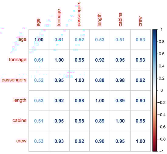
Figure 1.
Correlation plot for cruise ship info data.
Table 20.
Variance inflation factor values for cruise ship info data.
Finally, a regression model was fitted to the data using the OLS and different ridge estimators, and the results are listed in Table 21. From this table, one can see that the ridge estimators, existing as well as the proposed ones, had the smallest MSEs compared to the OLS estimator. In addition, our proposed estimators outperformed all the existing ridge estimators. Within our proposed estimators, The superior performance of NIS3 is evident as it produced lower MSEs than NIS1 and NIS2 Table 21.
Table 21.
Mean square error for different estimators of cruise ship info data (superscript represents ranks).
5.2. Economic Survey Data of Pakistan
We examined another dataset extracted from [] to assess the performance of the proposed estimators. The data set has a dependent variable Y that denotes the number of persons employed (in millions). The independent variables are Z1 = land cultivated (in millions of hectares); Z2 = inflation rate (in %); Z3 = number of establishments; Z4 = population (in millions); and Z5 = literacy rate (in %). From Table 22, one can see that variables are on different scales. For example, the variable Z1 ranges from 19.55 to 21.99, whereas Z3 ranges from 3248 to 5128. Therefore, the variables were standardized before the estimation of the model.
Table 22.
Descriptive statistics for economic survey data of Pakistan.
To check the linear association among the different variables of the data set, a correlation plot is given in Figure 2. This plot shows that the regressors are highly correlated. For example, the correlation between Z1 and Z3 is 0.94, whereas it is 0.98 between Z1 and Z4. Similarly, Z3 and Z4 have a correlation coefficient value of 0.96. The correlation coefficient values suggest that there may exist a serious problem of multicollinearity. To assess the strength of multicollinearity, VIF was calculated for the data, and the results are listed in Table 23. The table suggests that the regressors are strongly correlated and their VIF values are much higher. For example, the VIF value for Z1 is 32.144, which is an indication of a severe multicollinearity problem in the data.
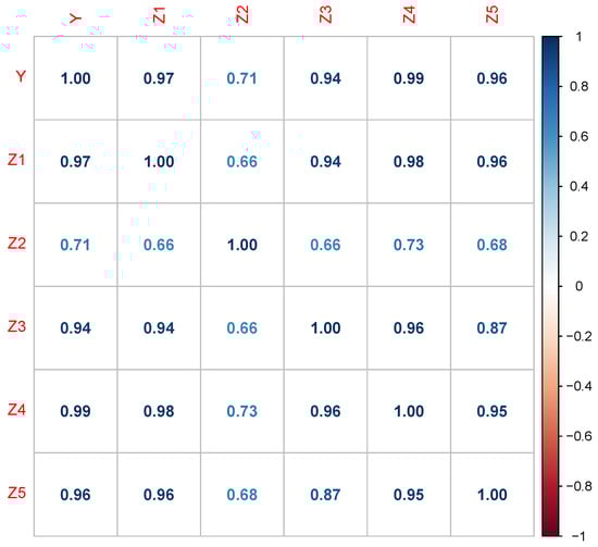
Figure 2.
Correlation plot for economic survey data of Pakistan.
Table 23.
Variance inflation factor values for economic survey data of Pakistan.
We fitted the following model to our data, and the results are listed in Table 24.
Table 24.
Meansquare error for different estimators of economic survey data of Pakistan (superscript represents ranks).
From this table, the poor performance of the OLS is evident, as it results in a larger MSE value compared to the ridge estimators. The proposed estimators performed relatively well compared to the existing ridge estimators, as NIS3 and NIS2 were ranked 1st and 2nd. Within the proposed estimators, NIS3 outperformed the other two proposals by producing a lower MSE value. From the simulation and real data analysis, it is concluded that the proposed estimators are efficient and can be used in a situation where strong multicollinearity exists in the data.
6. Conclusions
In this article, we proposed some new developments to the existing estimators of ridge parameters. Some of these existing estimators were modified, which resulted in three novel estimators of ridge parameters, which are NIS1, NIS2, and NIS3. The proposed estimators depend on the eigenvalues, the number of predictors, the standard deviation, and the number of observations. A simulation and real data study were conducted, and the performance of the ridge regression methods was evaluated on the basis of the mean squared error criterion. Based on the simulation results, the new proposed estimators NIS1, NIS2, and NIS3 were found to have the smallest MSEs in general. Comparing different parameter values, the simulation results suggested that the proposed estimators have the smallest MSEs than the OLS and existing ridge regression estimators. Finally, two real data sets were used to demonstrate the ability and the performance of the proposed estimators and it was found that the presented estimators performed relatively well compared to the existing ridge estimators by producing lower MSE values. From the simulation and real data analysis, it is concluded that the proposed estimators are efficient and can be used in a situation where strong multicollinearity exists in the data. Although the proposals perform relatively well compared to some of the existing estimators, more study is required before making any definite statement. In the future, some of the recently proposed ridge estimators from the literature can be compared with the proposed estimators to evaluate the proposals’ performance. Moreover, the theoretical properties of the proposed estimators can be studied in a future research work.
Author Contributions
Methodology, N.S. and I.S.; Software, I.S., A.A. and H.N.A.; Validation, S.A.; Formal analysis, N.S. and S.A.; Investigation, N.S.; Resources, A.A. and H.N.A.; Data curation, S.A. and H.N.A.; Writing-original draft, I.S. and A.A.; Visualization, N.S.; Supervision, I.S. All authors have read and agreed to the published version of the manuscript.
Funding
This research was funded by the Deanship of Scientific Research at Qassim University.
Data Availability Statement
The real data set used in the study is freely available from http://www.truecruse.com (accessed on 12 January 2022).
Acknowledgments
The researchers would like to thank the Deanship of Scientific Research, Qassim University for funding the publication of this project.
Conflicts of Interest
The authors declare no conflict of interest.
References
- Hoerl, A.E.; Kennard, R.W. Ridge regression: Applications to nonorthogonal problems. Technometrics 1970, 12, 69–82. [Google Scholar] [CrossRef]
- Muniz, G.; Kibria, B.G. On some ridge regression estimators: An empirical comparisons. Commun. Stat.—Simul. Comput. 2009, 38, 621–630. [Google Scholar] [CrossRef]
- Rajan, M. An efficient Ridge regression algorithm with parameter estimation for data analysis in machine learning. SN Comput. Sci. 2022, 3, 171. [Google Scholar] [CrossRef]
- Obenchain, R.L. Efficient generalized ridge regression. Open Stat. 2022, 3, 1–18. [Google Scholar] [CrossRef]
- Alkhamisi, M.A.; Shukur, G. Developing ridge parameters for SUR model. Commun. Stat.—Theory Methods 2008, 37, 544–564. [Google Scholar] [CrossRef]
- Yildirim, H.; Özkale, M.R. The performance of ELM based ridge regression via the regularization parameters. Expert Syst. Appl. 2019, 134, 225–233. [Google Scholar] [CrossRef]
- McDonald, G.C.; Galarneau, D.I. A Monte Carlo evaluation of some ridge-type estimators. J. Am. Stat. Assoc. 1975, 70, 407–416. [Google Scholar] [CrossRef]
- Michimae, H.; Emura, T. Bayesian ridge estimators based on copula-based joint prior distributions for regression coefficients. Comput. Stat. 2022, 37, 2741–2769. [Google Scholar] [CrossRef]
- Kibria, B.G. Performance of some new ridge regression estimators. Commun.-Stat.-Simul. Comput. 2003, 32, 419–435. [Google Scholar] [CrossRef]
- Alkhamisi, M.; Khalaf, G.; Shukur, G. Some modifications for choosing ridge parameters. Commun.-Stat.-Theory Methods 2006, 35, 2005–2020. [Google Scholar] [CrossRef]
- Muniz, G.; Kibria, B.; Shukur, G. On developing ridge regression parameters: A graphical investigation. Sort 2012, 36, 115–138. [Google Scholar]
- Månsson, K.; Shukur, G.; Golam Kibria, B. A simulation study of some ridge regression estimators under different distributional assumptions. Commun.-Stat.-Simul. Comput. 2010, 39, 1639–1670. [Google Scholar] [CrossRef]
- Kibria, B.; Lukman, A.F. A new ridge-type estimator for the linear regression model: Simulations and applications. Scientifica 2020, 2020, 9758378. [Google Scholar] [CrossRef] [PubMed]
- Arashi, M.; Valizadeh, T. Performance of Kibria’s methods in partial linear ridge regression model. Stat. Pap. 2015, 56, 231–246. [Google Scholar] [CrossRef]
- Clark, A.; Troskie, C. Ridge regression—A simulation study. Commun.-Stat.-Simul. Comput. 2006, 35, 605–619. [Google Scholar] [CrossRef]
- Ahn, J.J.; Byun, H.W.; Oh, K.J.; Kim, T.Y. Using ridge regression with genetic algorithm to enhance real estate appraisal forecasting. Expert Syst. Appl. 2012, 39, 8369–8379. [Google Scholar] [CrossRef]
- Shah, I.; Naz, H.; Ali, S.; Almohaimeed, A.; Lone, S.A. A New Quantile-Based Approach for LASSO Estimation. Mathematics 2023, 11, 1452. [Google Scholar] [CrossRef]
- Cule, E.; De Iorio, M. A semi-automatic method to guide the choice of ridge parameter in ridge regression. arXiv 2012, arXiv:1205.0686. [Google Scholar]
- Wong, K.Y.; Chiu, S.N. An iterative approach to minimize the mean squared error in ridge regression. Comput. Stat. 2015, 30, 625–639. [Google Scholar] [CrossRef]
- Hoerl, A.E.; Kannard, R.W.; Baldwin, K.F. Ridge regression: Some simulations. Commun.-Stat.-Theory Methods 1975, 4, 105–123. [Google Scholar] [CrossRef]
- Khalaf, G.; Shukur, G. Choosing ridge parameter for regression problems. Commun.-Stat.-Theory Methods 2005, 34, 1177–1182. [Google Scholar] [CrossRef]
- Ali, S.; Khan, H.; Shah, I.; Butt, M.M.; Suhail, M. A comparison of some new and old robust ridge regression estimators. Commun.-Stat.-Simul. Comput. 2021, 50, 2213–2231. [Google Scholar] [CrossRef]
- Shah, I.; Sajid, F.; Ali, S.; Rehman, A.; Bahaj, S.A.; Fati, S.M. On the performance of jackknife based estimators for ridge regression. IEEE Access 2021, 9, 68044–68053. [Google Scholar] [CrossRef]
- Pasha, G.; Shah, M. Application of ridge regression to multicollinear data. J. Res. (Sci.) 2004, 15, 97–106. [Google Scholar]
Disclaimer/Publisher’s Note: The statements, opinions and data contained in all publications are solely those of the individual author(s) and contributor(s) and not of MDPI and/or the editor(s). MDPI and/or the editor(s) disclaim responsibility for any injury to people or property resulting from any ideas, methods, instructions or products referred to in the content. |
© 2023 by the authors. Licensee MDPI, Basel, Switzerland. This article is an open access article distributed under the terms and conditions of the Creative Commons Attribution (CC BY) license (https://creativecommons.org/licenses/by/4.0/).