Optimisation of Cycling Trends in Hamiltonian Systems of Economic Growth Models

Abstract

The paper analyses dynamical growth models predicting the cyclic development of investigated economic factors. The provided research deals with an optimal control problem based on the economic growth model with the production function of Cobb–Douglas type. Following the Pontryagin maximum principle, we derived the Hamiltonian system and conducted its qualitative analysis, which reveals conditions for the cyclic behaviour of the optimal solutions around the isolate steady state. Numerical experiments visually illustrated the obtained results by demonstrating a phase portrait corresponding to a steady state of the focal type.

1. Introduction

The paper investigated stabilised solutions of an optimal control problem [1,2] that is based on an economic growth model [3,4]. More precisely, the work focused on the case when a steady state has the focal character and applies theoretical results [5,6] of a qualitative behaviour of the Hamiltonian systems to the specific growth model. At the end of the past and the beginning of the present century, optimal control problems found their wide application in economics [1,2,3,4]. This was caused by the usage of dynamical principles for designing economical models to predict scenarios of economic development (see [7]). Moreover, optimal control approaches have the opportunity to pursue a certain goal in the design of different scenarios of economic development and reveal the ways to achieve this goal by choosing specific control regimes (see [1,2,4,8]. For example, this goal can be the maximisation of the cumulative consumption level, the maximisation of an output, or cost optimisation. Often, models are aimed at constructing long-term forecasts that lead to the analysis of the corresponding control problems at the infinite time interval and to the study of the limit character of the optimal trends [1,9,10,11]. Therefore, we concentrated on the limit behaviour of an optimal solution when time goes to infinity. The present paper describes a classical growth model [1,2,3,4] and analysed conditions under which the economic development of some region has the cyclic character. The research operated with the Hamiltonian systems arising in the Pontryagin maximum principle, which was applied to a control problem of an optimal distribution of investments directed to the production factors. Production factors determine the output by means of the production function. The quality of the control process is estimated by the integral consumption index of logarithmic type discounted on the infinite time interval [1,3,8,10,12]. In these types of problems, the Jacobi matrix of a Hamiltonian system has a property that allows for making twice less the degree of its characteristic polynomial (see [5,6,13]). Using this property, we derived the condition for a cyclic behaviour of optimal trajectories around an isolate steady state. It is worth mentioning the previous works [2,9,10,14] that deal with a steady state having a saddle character. The paper is organized as follows: the next section describes a growth model and poses the problem, then we construct the Hamiltonian function and discuss its properties. The third section analyses the corresponding Hamiltonian system and its Jacobian. Using properties of the Jacobi matrix, we investigated conditions for the focal character of a steady state. As an example, we provide a numerical example illustrating theoretical results.

2. Growth Model

The paper investigated an optimal control problem that is based on an economic growth model aimed at the analysis of the gross domestic product (GDP) $Y=Y\left(t\right)$, depending on production factors such as capital stock $K=K\left(t\right)$ and labour $L=L\left(t\right)$, where parameter t stands for time. The relationship between the output (GDP) and the production factors is determined by the production function $Y=f(K,L)$.

Labour $L=L\left(t\right)$ is a share of the employed population of a region P [4], i.e., $L=E·P$, where the positive coefficient $E=E\left(t\right)$ is the labour efficiency. The capital dynamics depends on savings $S=S\left(t\right)$ and the positive capital depreciation rate $\delta$ (1):

$$\dot{K}\left(t\right)=S\left(t\right)-\delta K\left(t\right),K\left(0\right)=K_0.$$

(1)

The labour $L=L\left(t\right)$ changes due to the investments $R=R\left(t\right)$ in increasing the labour efficiency $E=E\left(t\right)$ (2):

$$\dot{L}\left(t\right)=bR\left(t\right),L\left(0\right)=L_0.$$

(2)

Under the condition of the closedness of the economy, for any moment of time t, investments $S\left(t\right)=u_1\left(t\right)Y\left(t\right)$ and $R\left(t\right)=u_2\left(t\right)Y\left(t\right)$ cannot exceed the output; thus, we have the restrictions (3):

$$Y\left(t\right)>S\left(t\right)+R\left(t\right)=(u_1\left(t\right)+u_2\left(t\right))Y\left(t\right)⩾0\Rightarrow 0⩽u_1\left(t\right)+u_2\left(t\right)<1.$$

(3)

Shares $u_1\left(t\right)$ and $u_2\left(t\right)$ of GDP invested in the capital $K\left(t\right)$ and labour $L\left(t\right)$ are nonnegative. Moreover, we assume that there exist two nonnegative constants $a_1$ and $a_2$ such that (4):

$$0⩽u_1\left(t\right)⩽a_1<1,0⩽u_2\left(t\right)⩽a_2<1.$$

(4)

Let symbol $\mathcal{U}$ indicate the domain for investment shares $u={\left(u_1,u_2\right)}^{\top }$ $\mathcal{U}=[0,a_1]\times [0,a_2]$. Following the work [4], we suppose that the employed population exponentially grows, i.e., $\dot{P}\left(t\right)=\gamma P\left(t\right)$, where $\gamma$ is a positive growth rate.

Introduce relative variables $y\left(t\right)$, $x_1\left(t\right)$, $x_2\left(t\right)$ as GDP $Y\left(t\right)$, capital $K\left(t\right)$, and labour $L\left(t\right)$ per one worker (5), i.e.,:

$$y\left(t\right)=\frac{Y\left(t\right)}{P\left(t\right)},x_1\left(t\right)=\frac{K\left(t\right)}{P\left(t\right)},x_2\left(t\right)=\frac{L\left(t\right)}{P\left(t\right)}\equiv E\left(t\right).$$

(5)

Due to the property of the production function $Y=f(K,L)$ of positive homogeneity, in new variables it has the form (6):

$$y\left(t\right)=\frac{F\left(K\right(t),L(t\left)\right)}{P\left(t\right)}=f(x_1\left(t\right),x_2\left(t\right))=f\left(x\left(t\right)\right),$$

(6)

where symbol $x\left(t\right)$ denotes the vector of phase variables $x={\left(x_1,x_2\right)}^{\top }$.

The dynamics of per capita capital $x_1\left(t\right)$ and the labour efficiency $x_2\left(t\right)$ satisfy the Equations (7) and (8):

$${\dot{x}}_1\left(t\right)=u_1\left(t\right)y\left(t\right)-(\delta +\gamma )x_1\left(t\right),x_1\left(t_0\right)=x_1^0,$$

(7)

$${\dot{x}}_2\left(t\right)=b{u}_2\left(t\right)y\left(t\right)-\gamma x_2\left(t\right),x_2\left(t_0\right)=x_2^0.$$

(8)

It is assumed that the per capita output $y=f\left(x\right)$ has the properties commonly corresponding to a production function. Function $f\left(x\right)$ is a twice continuously differentiable, increasing, strictly concave function in its variables $x_1$ and $x_2$. The last property of strict concavity means the Hessian matrix (9) is negative definite:

$$H_f=\left(\begin{array}{cc}{f}_{x_1^2}^{″}\left(x\right)& f_{x_1{x}_2}^{″}\left(x\right)\\ f_{x_1{x}_2}^{″}\left(x\right)& f_{x_2^2}^{″}\left(x\right)\end{array}\right)<0.$$

(9)

Due to the closedness of the economy system (see (3)), we can derive the consumption level as the difference between total output and investments in capital and labour efficiency (10):

$$C\left(t\right)=Y\left(t\right)(1-u_1\left(t\right)-u_2\left(t\right)).$$

(10)

In relative variables, this equality can be rewritten as follows (11):

$$c\left(t\right)=\frac{C\left(t\right)}{P\left(t\right)}=y\left(t\right)(1-u_1\left(t\right)-u_2\left(t\right))\approx y\left(t\right)(1-u_1\left(t\right))(1-u_2\left(t\right)).$$

(11)

The estimate can be applied since the product $u_1·u_2$ has a higher order of smallness than $u_i$ ($u_i\in [0,a_i]\subset [0,1)$, $i\in \{1,2\}$).

Utility function is the integral index of logarithmic type discounted in the infinite time interval. This type of index measures the cumulative value of relative consumption, expressed in the currency of a region, adjusted for the amount of currency depreciation rate over the time (12).

$$J(·)=\underset{0}{\overset{+\infty }{\int }}{e}^{-\rho t}\left(ln(1-u_1\left(t\right))+ln(1-u_2\left(t\right))+lnf\left(x\right(t\left)\right)\right)dt,\rho >0.$$

(12)

Here (12), the positive parameter $\rho$ is a discount factor.

Proposition 1 (Assumption 1).

Population growth satisfies exponential law. Production F(K, L) is positive homogeneous of the first degree.

Based on the described model of economy development, one can pose the optimal control problem with the infinite horizon, where the investment shares $u_1$, $u_2$ in production factors $x_1$, $x_2$, respectively, play the role of control parameters.

Problem 1 (Optimal Control Problem).

The problem is to synthesise such control strategies, $u^0\left(t\right)={\left(u_1^0\left(t\right),u_2^0\left(t\right)\right)}^{\top }\in \mathcal{U}$, which maximise the utility function $J(·)$ (12) along the trajectories $x\left(t\right)={\left(x_1\left(t\right),x_2\left(t\right)\right)}^{\top }$ of the dynamical system (7) and (8).

3. Control Problem Analysis

The posed problem satisfies all conditions of the existence theorem [11,15], and the optimality conditions for the problems in the infinite time interval within the Pontryagin maximum principle [1] (Theorem 18.2, p. 171).

The Hamiltonian function of the optimal control problem has the form (13)

$$\begin{array}{c}\hfill \tilde{H}(t,x,u,\tilde{\psi })=e^{-\rho t}\left(ln(1-u_1)+ln(1-u_2)+lnf\left(x\right)\right)+\\ \hfill {\tilde{\psi }}_1(u_{1}f\left(x\right)-(\delta +\gamma )x_1)+{\tilde{\psi }}_2(b{u}_{2}f\left(x\right)-\gamma x_2).\end{array}$$

(13)

Here, the conjugate variables $\tilde{\psi }=({\tilde{\psi }}_1,{\tilde{\psi }}_2)$ determine the “shadow prices” of capital $x_1$ and labour efficiency $x_2$, respectively. However, for further analysis, we introduce adjusted “shadow prices” ${\psi }_1=e^{\rho t}{\tilde{\psi }}_1$, ${\psi }_2=e^{\rho t}{\tilde{\psi }}_2$ and rewrite the Hamiltonian function as follows: $\hat{H}(·)=e^{\rho t}\tilde{H}(·)$. This change of conjugate variables excludes time variable t from the Hamiltonian function (14),

$$\begin{array}{cc}\hfill \hat{H}(x,u,\psi )& =ln(1-u_1)+ln(1-u_2)+lnf\left(x\right)+{\psi }_1(u_{1}f\left(x\right)-\hfill \\ \hfill & (\delta +\gamma )x_1) + {\psi }_2(b{u}_{2}f\left(x\right)-\gamma x_2).\hfill \end{array}$$

(14)

According to [14], the Hamiltonian function $\hat{H}(x,u,\psi )$ (14) has the following properties:

P1.

The Hamiltonian $\hat{H}(x,u,\psi )$ (14) is strictly concave in control variables $u_1$ and $u_2$.

This property together with the compactness of the control domain U ensures the existence of maximum of the Hamiltonian in control variables.

P2.

The maximised Hamiltonian $H(x,\psi )$ can be constructed by the rule (15)

$$\begin{gathered} \begin{array}{c}H(x,\psi )=\underset{u\in \mathcal{U}}{max}\hat{H}(x,u,\psi )=\hat{H}(x,u^{ij},\psi ),\end{array} \\ {u}_{ij}^0=(u_{1i}^0,u_{2j}^0),(x,\psi )\in D_{ij}={\Delta }_1^i\cap {\Delta }_2^j,(i,j=1,2,3), \end{gathered}$$

(15)

where sets ${\Delta }_1^i$ and ${\Delta }_2^j$ are determined as follows (16):

$$\begin{array}{c}{\Delta }_1^1=\{(x,\psi ):{\psi }_{1}f\left(x\right)\le 1\},u_1=0;\hfill \\ {\Delta }_2^1=\{(x,\psi ):b{\psi }_{2}f\left(x\right)\le 1\},u_2=0;\hfill \\ {\displaystyle {\Delta }_1^2=\left\{(x,\psi ):1\le {\psi }_{1}f\left(x\right)\le A_1\right\},u_1^0=1-\frac{1}{{\psi }_{1}f\left(x\right)};}\hfill \\ {\displaystyle {\Delta }_2^2=\left\{(x,\psi ):1\le b{\psi }_{2}f\left(x\right)\le A_2\right\},u_2^0=1-\frac{1}{b{\psi }_{2}f\left(x\right)};}\hfill \\ {\displaystyle {\Delta }_1^3=\left\{(x,\psi ):{\psi }_{1}f\left(x\right)\ge A_1\right\},u_1^0=a_1;}\hfill \\ {\displaystyle {\Delta }_2^3=\left\{(x,\psi ):b{\psi }_{2}f\left(x\right)\ge A_2\right\},u_2^0=a_2.}\hfill \end{array}$$

(16)

Here, constant $A_i$ is equal to $A_i={(1-a_i)}^{-1},i\in \{1,2\}$. Thus, the maximised Hamiltonian $H(x,\psi )$ has nine branches $H_{ij}(x,\psi )$. Moreover, each branch is determined in the domain $D_{ij}$ under the controls $(u_{1i}^0,u_{2j}^0),i,j\in \{1,2,3\}$.

P3.

The maximised Hamiltonian $H(x,\psi )$ is a smooth function of its variables $x_1,x_2,{\psi }_1,{\psi }_2$.

P4.

The maximised Hamiltonian $H(x,\psi )$ is a strictly concave function in phase variables $x_1$ and $x_2$ for all positive values of the conjugate variables ${\psi }_1>0$, ${\psi }_2>0$ in any domains $D_{ij},i,j=1,2,3$ except the domain $D_{22}$ of the non-constant control regime $\left(u_{12}^0,u_{22}^0\right)$. In domain $D_{22}$, strict concavity of the maximised Hamiltonian takes place if the matrix $\partial f$ is negative definite (17):

$$\partial f\left(x\right)=\left(\begin{array}{ccc}\hfill -f\left(x\right)& \hfill f_{x_1}^{\prime }\left(x\right)& \hfill f_{x_2}^{\prime }\left(x\right)\\ \hfill f_{x_1}^{\prime }\left(x\right)& \hfill f_{x_1^2}^{″}\left(x\right)& \hfill f_{x_1{x}_2}^{″}\left(x\right)\\ \hfill f_{x_2}^{\prime }\left(x\right)& \hfill f_{x_1{x}_2}^{″}\left(x\right)& \hfill f_{x_2^2}^{″}\left(x\right)\end{array}\right)\forall (x,\psi )\in D_{22},{\psi }_1>0,{\psi }_2>0.$$

(17)

The mentioned properties of the maximised Hamiltonian $H(x,\psi )$ guarantee that the necessary optimality conditions (in [1]) are sufficient for the optimality [2,9].

4. Hamiltonian System

According to the Pontryagin maximum principle, we construct the Hamiltonian system by the rule (18):

$${\dot{x}}_i\left(t\right)=\frac{\partial H\left(x\right(t),\psi (t\left)\right)}{\partial {\psi }_i},{\dot{\psi }}_i\left(t\right)=\rho {\psi }_i\left(t\right)-\frac{\partial H\left(x\right(t),\psi (t\left)\right)}{\partial x_i},i=1,2,3.$$

(18)

Applying formulae (18) to the investigated problem, the Hamiltonian system has the form (19):

$$\left\{\begin{array}{cc}{\dot{x}}_1\left(t\right)\hfill & =u_1^0\left(t\right)f\left(x\left(t\right)\right)-(\delta +\gamma )x_1\left(t\right)=G_1(x\left(t\right),\psi \left(t\right))\hfill \\ \\ {\dot{x}}_2\left(t\right)\hfill & =b{u}_2^0\left(t\right)f\left(x\left(t\right)\right)-\gamma x_2\left(t\right)=G_2(x\left(t\right),\psi \left(t\right))\hfill \\ \\ {\dot{\psi }}_1\left(t\right)\hfill & {\displaystyle =(\delta +\gamma +\rho ){\psi }_1\left(t\right)-f_{x_1}^{\prime }\left(x\left(t\right)\right)\left(\frac{1}{f\left(x\right(t\left)\right)}+u_1^0\left(t\right){\psi }_1\left(t\right)+b{u}_2^0\left(t\right){\psi }_2\left(t\right)\right)=}\hfill \\ & G_3(x\left(t\right),\psi \left(t\right))\hfill \\ \\ {\dot{\psi }}_2\left(t\right)\hfill & {\displaystyle =(\gamma +\rho ){\psi }_2\left(t\right)-f_{x_2}^{\prime }\left(x\left(t\right)\right)\left(\frac{1}{f\left(x\right(t\left)\right)}+u_1^0\left(t\right){\psi }_1\left(t\right)+b{u}_2^0\left(t\right){\psi }_2\left(t\right)\right)=}\hfill \\ & G_4(x\left(t\right),\psi \left(t\right)).\hfill \end{array}\right.$$

(19)

Relying on the results in [14], the steady state may exist in any domain $D_{ij}$ with non-zero controls, i.e., $i,j⩾2$. We pay attention to the case in which a steady state belongs the domain of variable controls $D_{22}$, which is described by the formula (20):

$$D_{22}=\left\{(x,\psi ):1\le {\psi }_{1}f\left(x\right)\le \frac{1}{1-a_1},1\le b{\psi }_{2}f\left(x\right)\le \frac{1}{1-a_2}\right\}.$$

(20)

The Hamiltonian system in the domain $D_{22}$ (20) has the form (21):

$$\left\{\begin{array}{cc}{\dot{x}}_1\left(t\right)\hfill & {\displaystyle =f\left(x\left(t\right)\right)-(\delta +\gamma )x_1\left(t\right)-\frac{1}{{\psi }_1\left(t\right)}=}\hfill \\ \hfill & G_1(x\left(t\right),\psi \left(t\right))\hfill \\ {\dot{x}}_2\left(t\right)\hfill & {\displaystyle =bf\left(x\left(t\right)\right)-\gamma x_2\left(t\right)-\frac{1}{{\psi }_2\left(t\right)}=}\hfill \\ \hfill & G_2(x\left(t\right),\psi \left(t\right))\hfill \\ {\dot{\psi }}_1\left(t\right)\hfill & {\displaystyle =(\delta +\gamma +\rho ){\psi }_1\left(t\right)-\left({\psi }_1\left(t\right)+b{\psi }_2\left(t\right)-\frac{1}{f\left(x\right(t\left)\right)}\right)f_{x_1}^{\prime }\left(x\left(t\right)\right)=}\hfill \\ \hfill & G_3(x\left(t\right),\psi \left(t\right))\hfill \\ {\dot{\psi }}_1\left(t\right)\hfill & {\displaystyle =(\gamma +\rho ){\psi }_2\left(t\right)-\left({\psi }_1\left(t\right)+b{\psi }_2\left(t\right)-\frac{1}{f\left(x\right(t\left)\right)}\right)f_{x_2}^{\prime }\left(x\left(t\right)\right)=}\hfill \\ \hfill & G_4(x\left(t\right),\psi \left(t\right)).\hfill \end{array}\right.$$

(21)

Next, we provide a qualitative analysis of the system (21) assuming the existence of an isolated steady state belonging the domain of variable control regime $D_{22}$.

Remark 1.

For the model with the Cobb–Douglas production function $y=f\left(x\right)=:\mu x_1^{\alpha }{x}_2^{\beta }$, a steady state $(x^{\ast },{\psi }^{\ast })$ does always exist (see [14]). The same work provides sufficient conditions guaranteeing belongingness of the steady state $(x^{\ast },{\psi }^{\ast })$ to the domain $D_{22}$ (20).

Proposition 2.

Let the system (21) have the only steady state $(x^{\ast },{\psi }^{\ast })$ and the following conditions on the maximum level of investment shares take place (22):

$$a_c\le a_1<1,a_c\le a_2<1,\mathit{where}{a}_c=\frac{\delta +\gamma }{\delta +\gamma +\rho };$$

(22)

then, the steady state $(x^{\ast },{\psi }^{\ast })$ belongs the domain of variable control regime $D_{22}$ (20).

Remark 2.

The steady state $x^{\ast }$ and the corresponding controls $(u_1^{\ast },u_2^{\ast })$ satisfying (22) and equal to the following values (23),

$$u_1^{\ast }=(\delta +\gamma )\frac{x_1^{\ast }}{f\left(x^{\ast }\right)},u_2^{\ast }=\frac{\gamma }{b}\frac{x_2^{\ast }}{f\left(x^{\ast }\right)},$$

(23)

are an equilibrium solution of the optimal control problem.

The next step is to determine a type of the steady state $(x^{\ast },{\psi }^{\ast })$.

4.1. Qualitative Analysis of a Steady State

Within the qualitative analysis of the Hamiltonian system, let us calculate Jacobi matrix J (24) at the steady state $(x^{\ast },{\psi }^{\ast })$.

$$\begin{array}{c}\hfill J=\left(\begin{array}{cc}\partial G_x^1& \partial G_{\psi }^1\\ \partial G_x^2& \partial G_{\psi }^2\end{array}\right),\end{array}$$

(24)

where partial derivatives (25) are:

$$\begin{array}{cc}\hfill \partial G_x^1& ={\left\{\frac{\partial G_i(x^{\ast },{\psi }^{\ast })}{\partial x_j}\right\}}_{i,j=1}^2,\partial G_{\psi }^1={\left\{\frac{\partial G_i(x^{\ast },{\psi }^{\ast })}{\partial {\psi }_j}\right\}}_{i,j=1}^2,\\ \hfill \partial G_x^2& ={\left\{\frac{\partial G_{2+i}(x^{\ast },{\psi }^{\ast })}{\partial x_j}\right\}}_{i,j=1}^2,\partial G_{\psi }^2={\left\{\frac{\partial G_{2+i}(x^{\ast },{\psi }^{\ast })}{\partial {\psi }_j}\right\}}_{i,j=1}^2.\end{array}$$

(25)

Partial derivatives of the right-hand parts $G_i(x,\psi ),(i=1,\dots ,4)$ of the system (21) satisfy Formulae (26):

$$\begin{array}{cc}\hfill \partial G_x^1& =\left(\begin{array}{cc}{f}_{x_1}^{\prime }& f_{x_2}^{\prime }\\ b{f}_{x_1}^{\prime }& b{f}_{x_2}^{\prime }\end{array}\right)-\left(\begin{array}{cc}\delta +\gamma & 0\\ 0& \gamma \end{array}\right),\hfill \\ \hfill \partial G_{\psi }^1& ={\left(\begin{array}{cc}{\psi }_1^{\ast }& 0\\ 0& {\psi }_2^{\ast }\end{array}\right)}^{-2},\hfill \\ \hfill \partial G_{\psi }^2& =-{\left(\partial G_x^1\right)}^T+\rho E_2\hfill \\ \hfill \partial G_x^2& {\displaystyle =-\frac{1}{f^2\left(x^{\ast }\right)}\left(\begin{array}{cc}{\displaystyle {\left(f_{x_1}^{\prime }\right)}^2}& f_{x_1}^{\prime }{f}_{x_2}^{\prime }\\ f_{x_1}^{\prime }{f}_{x_2}^{\prime }& {\displaystyle {\left(f_{x_2}^{\prime }\right)}^2}\end{array}\right)-}\hfill \\ \hfill & \left({\displaystyle {\psi }_1^{\ast }+b{\psi }_2^{\ast }-\frac{1}{f\left(x^{\ast }\right)}}\right)\left(\begin{array}{cc}{f}_{x_1^2}^{″}\left(x^{\ast }\right)& f_{x_1{x}_2}^{″}\left(x^{\ast }\right)\\ f_{x_1{x}_2}^{″}\left(x^{\ast }\right)& f_{x_2^2}^{″}\left(x^{\ast }\right)\end{array}\right).\hfill \end{array}$$

(26)

Jacobi matrix (26) has some useful properties for estimating its eigenvalues. These properties are based on the notion of the Hamiltonian matrix. There are several equivalent definitions of a Hamiltonian matrix; however, for the considered problem the next definition is more convenient to use.

Definition 1.

A block matrix M of the form $M={\left(\begin{array}{cc}A& B\\ C& -A^{\top }\end{array}\right)}_{2n\times 2n}$ is said to be Hamiltonian if its blocks B and C are symmetric sub-matrices.

The most valuable properties of a Hamiltonian matrix are listed below.

 PH1. 

Characteristic polynomial is an even function.

 PH2. 

Eigenvalues of a Hamiltonian matrix are symmetric with respect to the imaginary axis.

 PH3. 

If blocks B and C are positive-definite matrices then the Hamiltonian matrix M does not have purely imaginary eigenvalues (see [13]).

 PH4. 

If blocks B and C are positive definite matrices then the determinant of the Hamiltonian matrix M satisfies the inequality (see [5]): ${(-1)}^{n}detM⩾detBdetC>0.$

In [5], the authors proved that the Jacobi matrix J (24)–(26) of the considered problem can be represented as the sum of Hamiltonian and diagonal matrices, i.e., ${\displaystyle J=M+\rho /2E_4}$. Consequently, the eigenvalues of the Jacobi matrix and the Hamiltonian matrix are tied to equality ${\lambda }_J={\lambda }_M+\rho /2$. Blocks $\partial G_{\psi }^1$ and $\partial G_x^2$ of the Jacobi matrix (24)–(26) are positive definite due to the property P4 of the maximised Hamiltonian function $H(x,\psi )$. Hence, the Hamiltonian matrix $M=J-\rho /2E_4$ does not have purely imaginary eigenvalues. Finally, one can derive explicit formulae for eigenvalues of the Jacobi matrix using the corresponding Hamiltonian matrix.

Theorem 1.

Characteristic polynomial $det(J-\lambda E_4)=0$ of the Jacobi matrix J (24) can be reduced to the form (27):

$${\tau }^2+a_2\tau +a_4=0,a_2=-\frac{\mathrm{tr}{M}^2}{2}<0,a_4=\frac{1}{4}(2a_2^2-\mathrm{tr}{M}^4)=detM>0,$$

(27)

where new variable τ is related to λ by the equality $\tau ={(\lambda -\rho /2)}^2$. Analysis of the quadratic polynomial (27) implies that four eigenvalues of the Jacobi matrix are found by the formula (28):

$${\lambda }_{1,2,3,4}=\left\{\begin{array}{cc}\pm \sqrt{{\tau }_{1,2}}+\rho /2,& if{a}_2^2⩾4a_4,\hfill \\ \sqrt{r}\left(\pm cos(\phi /2)\pm isin(\phi /2)\right)+\rho /2,& if{a}_2^2<4a_4,\hfill \end{array}\right.$$

(28)

where ${\tau }_{1,2}=\left(-a_2\pm \sqrt{a_2^2-4a_4}\right)/2$, $r=\sqrt{a_4}$ and $\phi =arctan\sqrt{4a_4/a_2^2-1}$.

Next, we performed the analysis of the model parameters which cause the cyclic behaviour of the optimal trajectories around the steady state. In other words, we paid attention to the case in which the discriminant $D=a_2^2-4a_4$ of the quadratic Equation (27) is strictly negative.

4.2. Numerical Results for Cobb-Douglass Production Function

Let us consider the Cobb–Douglas production function of the form $y=f\left(x\right):=\mu x_1^{\alpha }{x}_2^{\beta }$, where parameters $\alpha$, $\beta$, and their sum $\alpha +\beta$ belong to interval $(0,0.5)$. In [14], one can find a detailed analysis of this problem with the Cobb–Douglas production function. We focused on the analysis of the discriminant D as a function of model parameter $\rho$. Elements of the matrix M in (27) depend on $\rho$, thus (29):

$$D\left(\rho \right)=a_2^2-4a_4=\mathrm{tr}{M}^4-\frac{1}{2}{\mathrm{tr}}^2{M}^2,\mathrm{where}M=M\left(\rho \right).$$

(29)

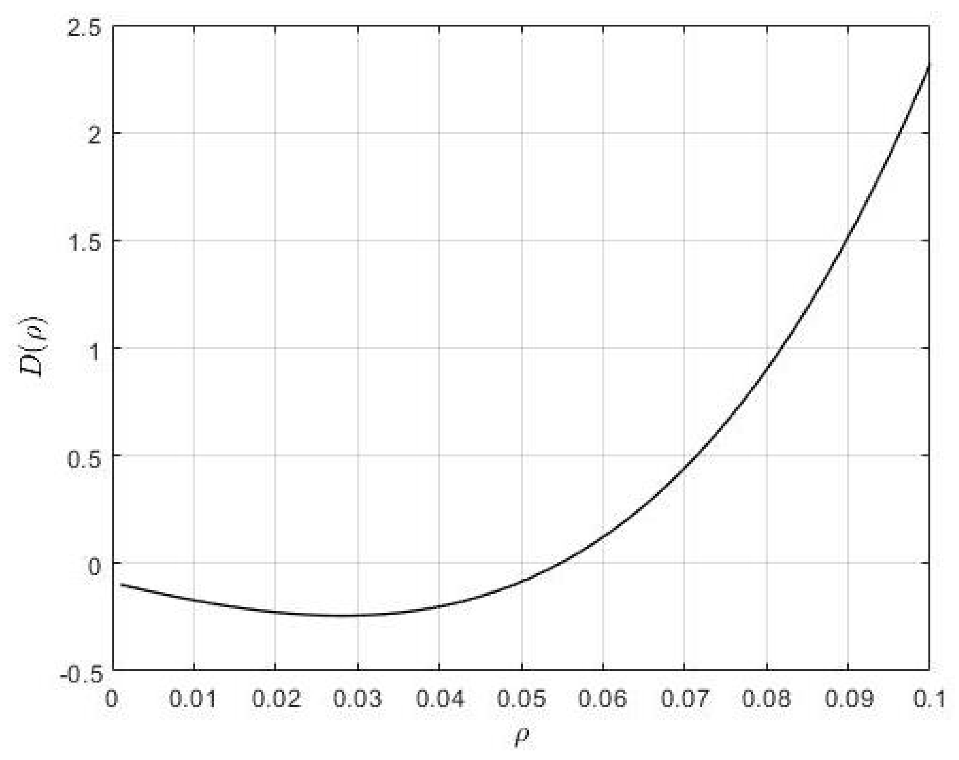
Figure 1 demonstrates the discriminant as a function of the discount factor $\rho$. One can see that there exists a range for the parameter $\rho$, when the discriminant $D=D\left(\rho \right)$ is strictly negative. According the experimental data, this range can be estimated as $(0,0.055)$. Selecting parameter $\rho$ at the level of $5\%$, we solved the Hamiltonian system stabilised (see [5,6]) around the steady state. 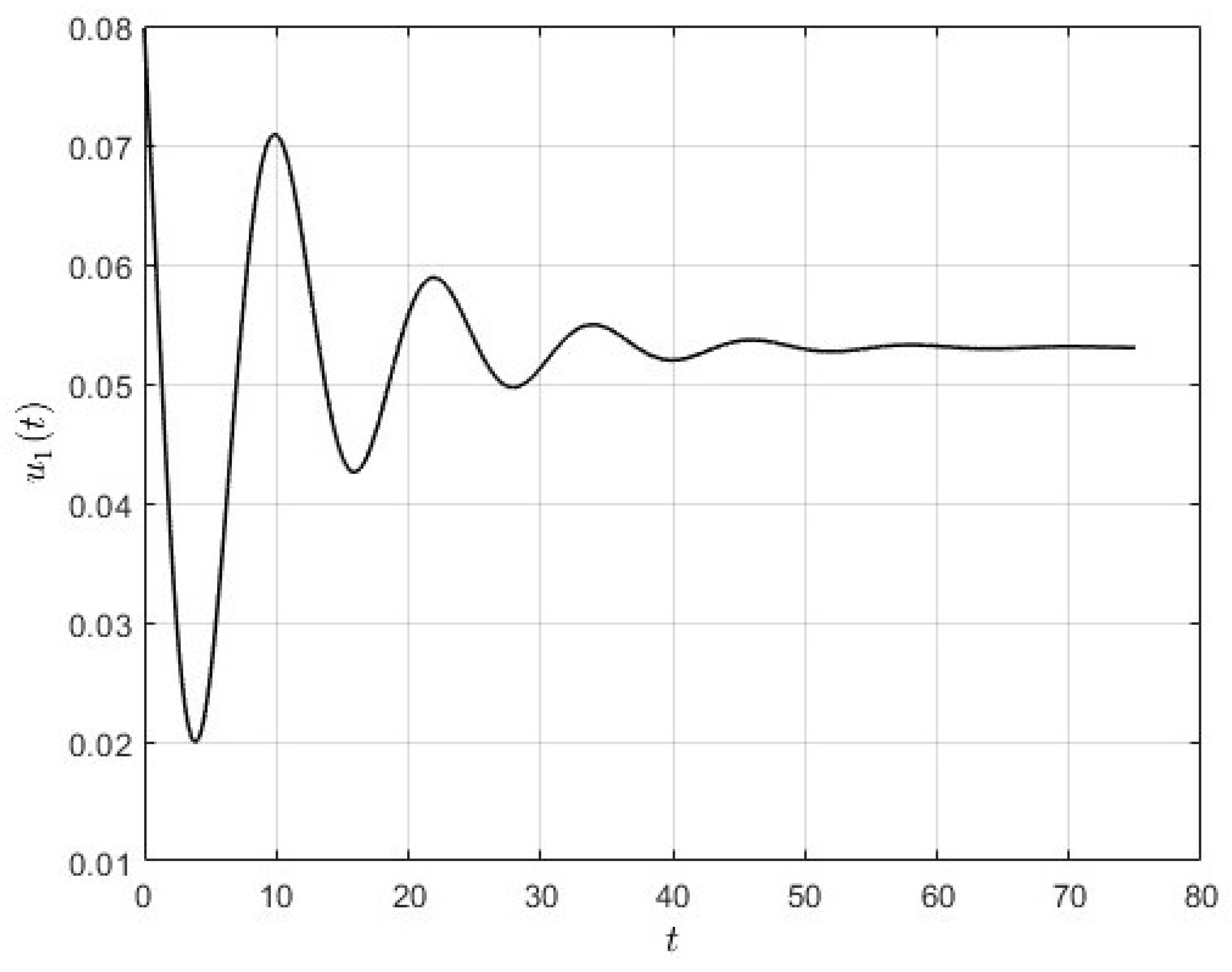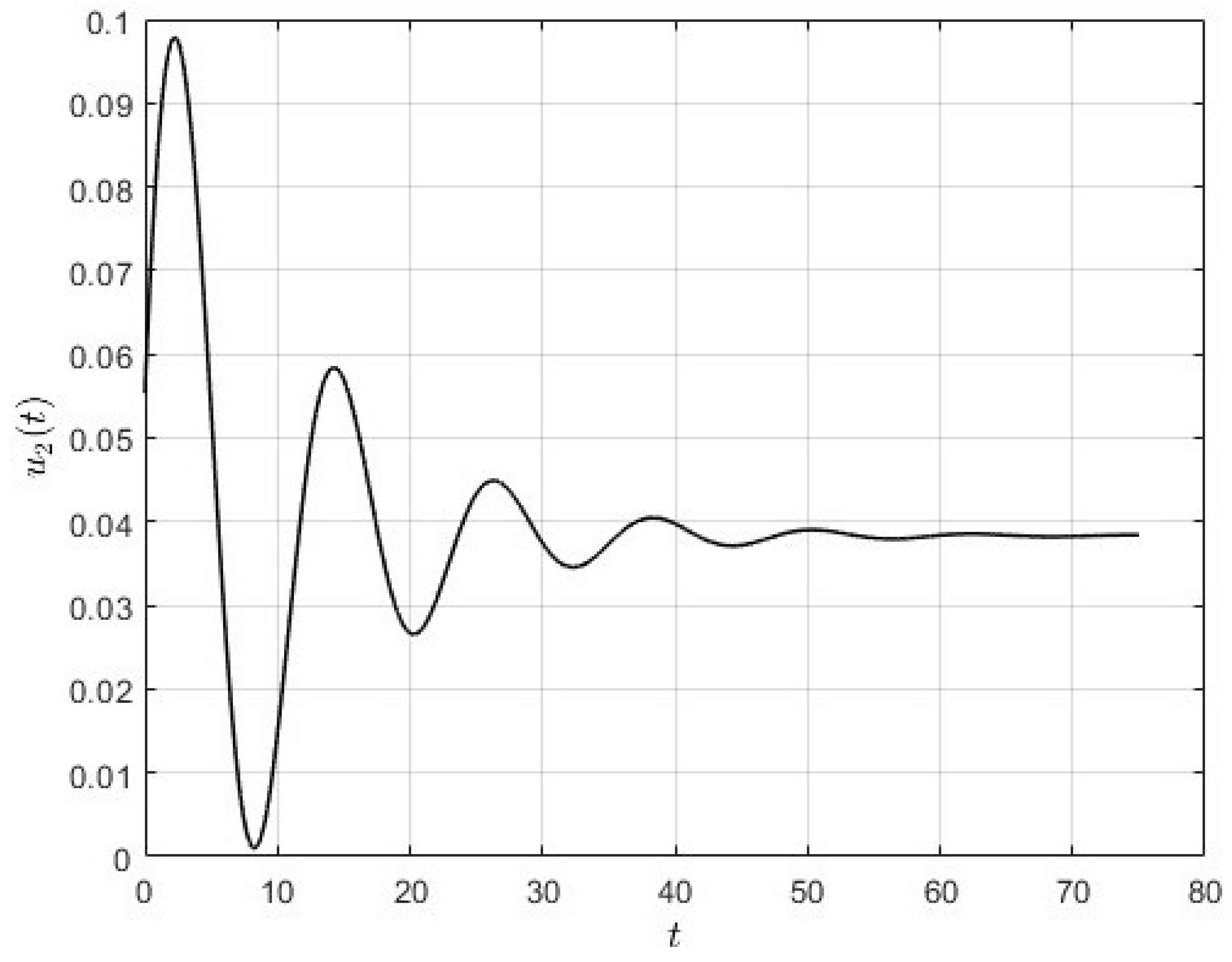One can see the phase portrait of the stabilised solution in Figure 2. Obviously, the phase trajectory has a spiral-form cyclically converging to the steady state. Thus, under the small values of the discount factor, optimal trends of the growth model may behave cyclically. Here, we provide numerically the effect of time-dependent control on the system by the values of $u_1\left(t\right)$ and $u_2\left(t\right)$ (Figure 3 and Figure 4), which are given in Equation (16) for the Cobb–Douglas production function in the focal equilibrium (see (23)).

5. Conclusions

The paper described the two-factors growth model behaving in a cyclic way under some values of the discount factor. Based on the qualitative analysis of the Hamiltonian system and its relation with the Hamiltonian matrix, we explicitly found the eigenvalues of the Jacobi matrix. It provides the possibility of considering the discriminant of the characteristic polynomial as a function of the chosen parameter (in this case, it is the discount factor). Next, performing a numerical analysis of the discriminant function, we estimated the range of the cyclic behaviour of the system. Finally, solving the stabilised Hamiltonian system with the parameter selected from the obtained range, we are convinced that the trajectory has a spiral form.