Reliability Analysis of High-Voltage Drive Motor Systems in Terms of the Polymorphic Bayesian Network

Abstract

The reliability of the high-voltage drive motor system for pure electric commercial vehicles is in premium demand. Conventional reliability based on fault tree analysis methods is not suitable for the quantitative assessment of polymorphic systems. As an example of a pure electric commercial vehicle, this paper combines polymorphic theory and Bayesian theory to establish a polymorphic Bayesian network model of a high-voltage drive motor system in terms of a polymorphic fault tree and to quantitatively judge the system. The polymorphic Bayesian network (BN) model can accurately depict the high-voltage drive motor system’s miscellaneous fault states and solve the top event’s probability in every state, also solving the system and drawing the consistent conclusion that the presence of abrasive particles, high-temperature gluing, moisture, and localized high temperatures are the system’s weak links by solving the critical importance, probabilistic importance, and posterior probability of the underlying event, which provides a theoretical reference for structure contrive optimization and fault diagnosis. This is extremely important in terms of improving pure electric commercial vehicles’ high-voltage drive motor systems.

1. Introduction

Energy and environmental issues have worsened due to increased vehicle ownership. At current, major domestic and foreign manufacturers have focused their attention on energy-saving, environmentally friendly, and high-capacity pure electric commercial vehicles. According to statistical analysis of the GGII (Gao Gong Industrial Research Institute), from January to November 2022, domestic sales of new energy heavy commercial vehicles amounted to more than 19,000 units, a year-on-year increase of 155%, accounting for 6.2% of the entire heavy commercial vehicle market. In addition, for different types of new energy commercial vehicles, the proportion of pure electric heavy-duty commercial vehicles is also the largest. While pure electric commercial vehicles are being promoted, the number of accidents caused by the reliability of high-voltage drive motor systems is increasing every year; each accident is a harsh reality for the reliability of the high-voltage electrical systems of pure electric commercial vehicles. The complex operating conditions of pure electric commercial vehicles require drive motors that can perform frequent start–stop and acceleration–deceleration characteristics and work reliably in harsh environments. Therefore, high-voltage drive motor systems have high requirements for reliability, cooling performance, energy density, adaptability, etc.

Reliability analysis techniques have achieved extensive use in the expanding area of engineering. Watson et al. first proposed fault tree analysis (FTA) [1]. Following this, Hasse et al. [2] studied and generalized the FTA algorithm, which made the reliability analysis method not limited to a single FTA. Cao et al. [3] combined fault tree analysis and binary decision diagram (BDD) methods which solved the problem of “combinatorial explosion” results by applying fault tree analysis methods only in fault diagnosis. Li et al. [4] put forward a decision tree based on the method for line fault cause analysis by mining fault causes’ time distribution law and the hierarchical structure from fault history, which improved the analysis speed, provided more detailed and accurate conclusions, and illustrated the effectiveness of the algorithm by providing examples. Jiao M et al. [5] transformed the fault tree (FT) into a state transition diagram (STD) to simplify the FT. Multiple fault combinations can be diagnosed and unnecessary operations can be reduced by using the converted STD to handle intermediate and basic events separately when performing fault diagnosis. Waghen K et al. [6] suggested multi-level interpretable logic tree analysis (MILTA) for the fault-level causal analysis of complex systems based on typical fault datasets.

As the complexity of the analysis system becomes progressively greater, the restrictions of traditional FTA methods for the ambiguity of the occurrence of base events are revealed. Using fuzzy probabilities instead of exact probabilities, fuzzy fault tree analysis (FFTA) solves probabilistic uncertainty in fault tree analysis. It was initially put forward by Tanaka et al. [7]. By creating a FFT model for excavation workings and gas explosion in coal mining, Shi et al. [8] determined the FT’s minimum path and minimum cut set and evaluated the significance of the fault tree configuration. The probability of gas explosion is calculated, which provides a theoretical basis for the preparation and prevention of coal mine accidents. Nadjafi et al. [9] put forward a fault tree reliability analysis method for complex engineering systems based on fuzzy time-to-failure (FTTF), which showed significant advantages of high accuracy and low workload in aerospace emergency detection systems. By introducing a fuzzy structured element-based method, Cui et al. [10] used the discrete space fault tree (DSFT) to establish an element discrete space fault tree (EDSFT). The element-based EDSFT method can maintain the original fault data’s distribution features and lay the groundwork for analyzing large error data, making it appropriate for system reliability analysis when large fault data and multiple factors are at play. Li et al. [11] performed a gas turbine fuel system fuzzy fault tree analysis by combining fuzzy information with the FT from staff feedback to improve the reliability of some components of the system. The theoretical basis was provided for subsequent system design and performance improvement. Yu [12] analyzed the weakest t-norm ($T_{\omega }$) to propose an FFT based on this and derived reliable probability through the evaluation of domain experts. This method is combined with the traditional submarine pipeline leakage failure probability risk assessment method. The results showed that the method has good validity and applicability.

In the practical field of engineering, the state of the system and the bottom events also show polymorphism. In addition, the reliability analysis of intricate polymorphic systems cannot be solved using the straightforward fuzzy fault tree analysis method. Belief networks (BNs) were first introduced by Pearl [13] in 1986 and have been used to deal with uncertain knowledge and polymorphism problems in subsequent developments. Portinale and Bobbio [14] performed a reliability analysis of a digital control system using Bayesian networks (BNs). Mahadevan et al. [15] compared traditional reliability analysis methods with Bayesian networks for parallel and series systems and verified their effectiveness. Liu [16] presented a fuzzy reliability estimation approach in terms of a belief network and T-S (Takagi–Sugeno) FT to evaluate the fuzzy reliability of the injection system. The method solved the problems of difficulty in constructing conditional probabilities for Bayesian network nodes, the difficulty of obtaining accurate fault probability data, and the inability of T-S fault tree analysis methods to reason backwards and provided a basis for improving system reliability and error judgment. Fuzzy mathematical principles and grey system principles were introduced into Bayesian networks by Wang et al. [17], who established a grey fuzzy Bayesian network model and proposed a reliability analysis method for intricate ambiguity multi-state systems with uncertainty affiliation functions and interval eigenvalues. Feng et al. [18] developed a crane reliability analysis model based on BNs under expert evaluation and verified the validity. Guo et al. [19] used a discrete Bayesian network to present a dynamic system reliability analysis model with common cause failure. A digital safety level distributed control system of a nuclear power plant was applied to verify the validity of this model. Li et al. [20] used BNs to analyze offshore floating wind turbines’ reliability to predict the average failure time and system failure rate. The failure rate’s prediction error is about one-third of the FTA’s prediction error. Bayesian networks are capable of handling uncertainty information. The root nodes in a polymorphic Bayesian network can represent discrete and continuous variables of two or more states, the conditional probability distribution between neighboring nodes can represent deterministic and uncertain logical relationships between variables, and the leaf nodes can be used to represent the top-of-failure events of the system, which is a great advantage in solving probabilistic problems of uncertainty. The research based on the reliability method of polymorphic systems has achieved remarkable results in both theoretical innovation and practical engineering application, and after continuous development, the reliability analysis of polymorphic systems has been used in various engineering fields, e.g., the fatigue analysis of mechanical parts [21,22], rail transit systems [23], mechanical structures and systems [24,25], risk assessment [26], and medical systems [27].

Of the many factors of the high-voltage drive motor system’s degraded-state mode, aging, corrosion, and deformation are multi-state events. When a common cause failure occurs between nodes, it leads to a complex Bayesian network structure, and it is too difficult to calculate the failure probability of the target nodes using Bayesian inference algorithms. Consequently, taking into account the logic between events and the polymorphic nature of the high-voltage drive motor system of pure electric commercial vehicles, only the reliability analysis of the system using polymorphic Bayesian networks under non-common cause failure is considered.

This work takes a pure electric commercial vehicle’s high-voltage drive motor system as the case study and applies the theory of polymorphic and Bayesian networks to establish a high-voltage drive motor system polymorphic Bayesian network model. The probabilities solved for the top event being in normal, degradation, and failure states are 0.9841, 0.00712, and 0.00878, respectively. In addition, the probability of solved for the system’s reliability is 0.9913. From the bottom event’s critical importance, probability importance, and the posterior probability of the presence of abrasive particles, high-temperature gluing, moisture, and localized high temperatures as critical events affecting the system failure were known.

In this paper, the following work has been accomplished: (1) the system’s FFT is built by taking a pure electric commercial vehicle’s high-voltage drive motor system as the case study. The transformation relationship between the Bayesian network and the FT is used to establish the system’s polymorphic Bayesian network model, and the occurrence probability in every state is solved by Bayesian network inference. (2) Through quantitative analysis, the system’s weakest links were identified from the view of the bottom event’s critical importance, probability importance and the posterior probability.

The polymorphic Bayesian network analysis’ basic principles are described in detail in Section 2 of this paper. Section 3 establishes and analyzes the high-voltage drive motor system polymorphic Bayesian network model for pure electric commercial vehicles. Section 4 solves the polymorphic Bayesian network model of the high-voltage drive motor system. Lastly, Section 5 is the conclusion, which summarizes the system reliability analysis in the previous chapters.

2. Reliability Analysis Methods in Terms of the Polymorphic Bayesian Networks

2.1. The Method of FTA

FTA [28] is the reliability analysis method that analyses all probable reasons for system failure and draws the “tree”, identifies the fundamental causes that lead to system breakdown through qualitative analysis, and calculates the top event’s failure probability and the basic events’ importance through quantitative analysis.

2.1.1. Top Event’s Probability

The top event’s probability is solved by quantitative analysis based on the structure function and the bottom event’s occurrence probability. Assume that $P\left(X_i\right)\left(i=1,2,\dots ,n\right)$ is the bottom event’s occurrence probability $X_i(i=1,2,\dots ,n)$. When the basic events’ occurrence is mutually independent, the probabilities of the top events under the “OR” and “AND” gates are as follows.

The probability of at least one basic event happening under the “OR” gate condition is:

$$P_{\cup }=1-\left\{\left[1-P\left(X_1\right)\right]\times \left[1-P\left(X_2\right)\right]\times \dots \times \left[1-P\left(X_n\right)\right]\right\}=1-{\displaystyle \prod _{i=1}^n\left[1-P\left(X_i\right)\right]}$$

(1)

where $P_{\cup }$ is the probability of at least one basic event happening, and $P\left(X_i\right)\left(i=1,2,\dots ,n\right)$ is the bottom event’s occurrence probability.

The basic events’ probability occurring in simultaneity under the “AND” gate condition is:

$$P_{\cap }=P\left(X_1\right)\times P\left(X_2\right)\times \dots \times P\left(X_n\right)={\displaystyle \prod _{i=1}^{n}P}\left(X_i\right)$$

(2)

where $P_{\cap }$ is the probability of n basic events occurring simultaneously.

2.1.2. Reliability of the System

From classical reliability theory, the formula for the relationship between the failure rate and reliability is:

$$R\left(t\right)=exp\left(-{\displaystyle {\int }_0^t\lambda }\left(t\right)dt\right)$$

(3)

While $\lambda \left(t\right)$ is a constancy, i.e., $\lambda \left(t\right)=\lambda$, and the system operating time t tends to unit 1. The system’s reliability is:

$$R\left(t\right)\approx exp\left(-\lambda \right)$$

(4)

From the fact that reliability and unreliability are opposing events, the formula between unreliability and the failure rate that can be obtained from Equation (4) is:

$$F\left(t\right)=1-R\left(t\right)=1-exp\left(-\lambda \right)$$

(5)

In Equation (5), $F\left(t\right)$ is the unreliability, $R\left(t\right)$ is the reliability, and $\lambda$ is the failure rate.

2.2. Polymorphic Fault Gate

The logic gate is referred to as a polymorphic fault gate when it comprises one or more polymorphic events which are contained in the input to the top event. $X_i(i=1,2,\dots ,n)$ with n being the polymorphic input events, that is, the input event satisfies $S_{X_i}\in \left\{0,0.5,1\right\}$, $S_{X_i}\in$ {normal,degradation,failure}. Indeed, the top event U conforms to Equation (6).

$$S_U=\left\{\begin{array}{cc}0& {\displaystyle \sum _{i=1}^n{S}_{X_i}=0}\\ 0.5& S_{X_i}\le 0.5 and{\displaystyle \sum _{i=1}^n{S}_{X_i}\ne 0}\\ 1& Others\end{array}\right.$$

(6)

Equation (6) indicates that the output events’ state is also normal for normal input polymorphic events, and when the state of the input polymorphic events is in the degradation state or a combination of normal and degradation, the output events are also in a degradation state. When at least one input polymorphic event is in failure, the system fails [29].

Table 1. The relationship between the states of the output events and the input of the polymorphic system.

I1	I2	O
0	0	0
0	0.5	0.5
0	1	1
0.5	0	0.5
0.5	0.5	0.5
0.5	1	1
1	0	1
1	0.5	1
1	1	1

shows the description of Equation (6).

In Table 1, I₁ and I₂ are the two input events. O is the output event. 0, 0.5, and 1 represent the three states of normal, degradation, and failure, respectively. In addition, there are only three states of input and output.

2.3. Basic Theory of Bayesian Networks

2.3.1. The Foundations of Bayesian Networks Theory

Bayesian networks are built on conditional probability, joint probability, and total probability.

• Conditional probability

For any two events X and Y and event X, the occurrence probability is non-negative, namely $P(X)>0$, and $P(Y|X)$ is the probability of event Y happening under the conditions of a given event X happening. The formula is expressed is:

$$P\left(Y|X\right)=\frac{P\left(XY\right)}{P\left(X\right)}$$

(7)

where $P\left(XY\right)$ is the probability of event X occuring simultaneously with event Y.

2.

Joint probability

For the probability of events X and Y happening at the same time, Equation (7) is used to obtain the probability:

$$P\left(XY\right)=P\left(X\right)•P\left(Y|X\right)$$

(8)

where $P\left(Y|X\right)$ is the probability of event Y occuring conditional on event X occuring.

3.

Total probability

Suppose $X_1,X_2,\dots ,X_n$ is a partition of the sample space X. Well, for any event Y, the chance of occurrence is:

$$P\left(Y\right)={\displaystyle \sum _{i=1}^{n}P\left(X_i\right)•P\left(Y|X_i\right)}$$

(9)

4.

Bayesian formula

The conditional probability and total probability are used to obtain:

$$P\left(X_i|Y\right)=\frac{P\left(X_i\right)P\left(Y|X_i\right)}{{\displaystyle \sum _{i=1}^{n}P\left(X_i\right)P\left(Y|X_i\right)}}$$

(10)

where $P\left(X_i|Y\right)$ is the posterior probability; $P\left(X_i\right)$ is the prior probability; $P\left(Y|X_i\right)$ is the likelihood probability [30]; $X_1,X_2,\dots ,X_n$ are mutually independent causes; and Y is the result. In practical engineering, prior probabilities and likelihood probabilities can be predicted. Using the Bayesian formula, it is possible to reason about the probability of the occurrence of a cause $P\left(X_i|Y\right)$ given the conditions under which the outcome occurs and to determine the cause that has the greatest influence on the outcome.

2.3.2. Bayesian Networks’ Basic Principles

$B=<G, P>=<<V, E>, P>$ represents Bayesian networks, which consists of conditional probability distribution (CPD) and a directed acyclic graph (DAG) [31,32]. Where $G=<V, E>$ represents the DAG, the elements in the node set V represent the variables, and E is the association between the variables [33,34]. In a directed acyclic graph of the BN, if nodes X to Y have a directed edge, then X is Y’s parent node. The parent node and children node of a node are called its neighbor node. There is no parent node for the root node and no children node for the leaf node. pa(X) or $\pi \left(X\right)$ represent the node X’s parent node, the children node is denoted as ch(X), and the neighbour node is denoted as nb(X) [35]. P in Bayesian networks denotes the conditional probability distribution and is represented by the conditional probability table (CPT) when the nodes are discrete random variables.

Semantically, a BN is a representation of the decomposition of the junction probability distribution. $X_1,X_2,\dots ,X_n$ are variables in the Bayesian network, and the joint probability distribution is:

$$P\left(X_1,X_2,\dots ,X_n\right)={\displaystyle \prod _{i=1}^{n}P\left(X_i|\pi \left(X_i\right)\right)}$$

(11)

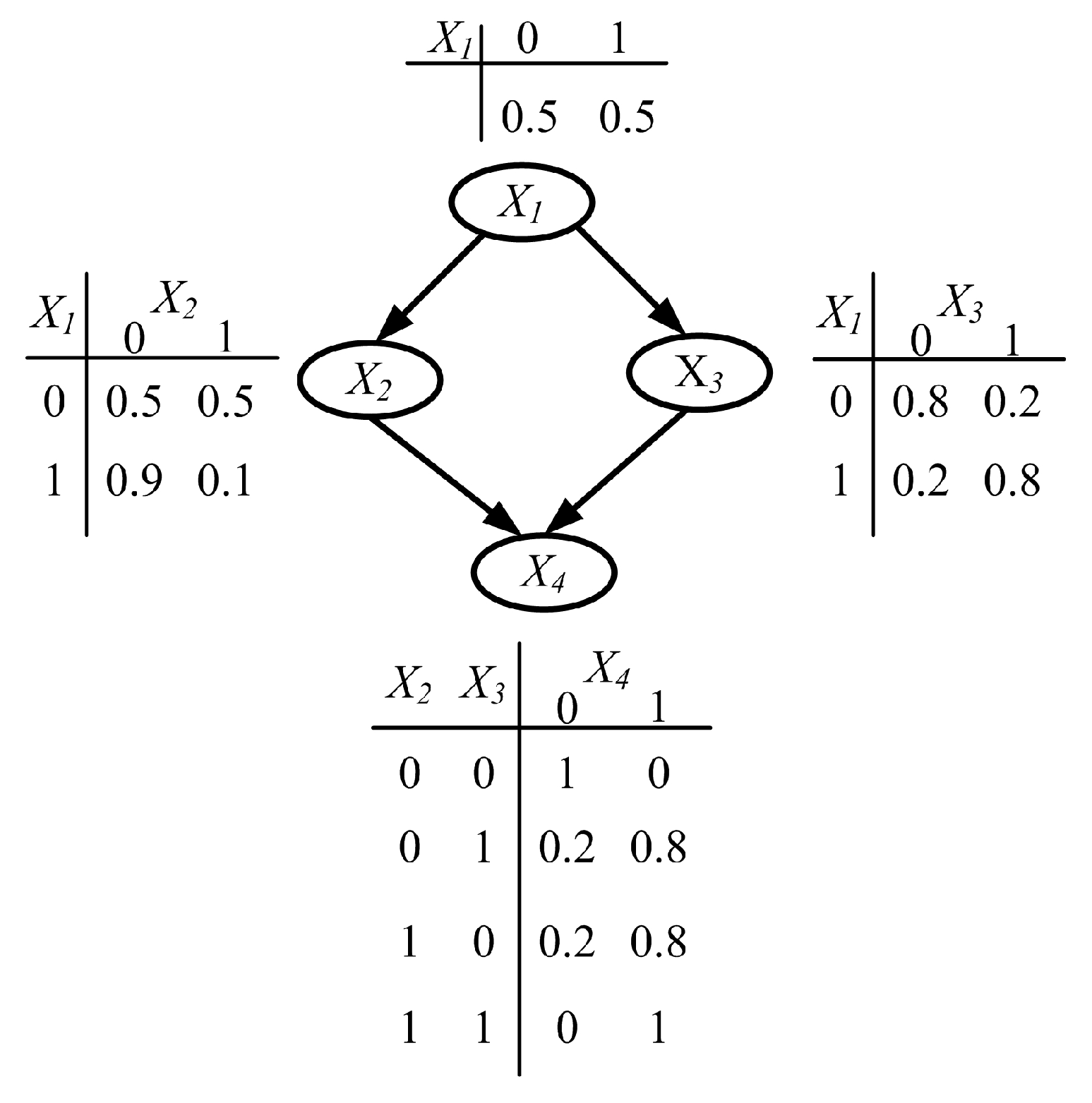
Figure 1 gives a simple example of a BN, in which X₁ is the root node and also X₂ and X_3′ parent nodes. X₄ is a leaf node and also the child node of X₂ and X₃. X₂ and X₃ represent the intermediate nodes. Next to the nodes is a table of conditional probabilities between the nodes. Each node in the Bayesian network has two states, 0 and 1, representing non-occurrence and occurrence, respectively.

According to Equation (11), the junction probability distribution function comprises all nodes in Figure 1 and is:

$$P\left(X_1,X_2,X_3,X_4\right)=P\left(X_4|X_2,X_3\right)P\left(X_2|X_1\right)P\left(X_3|X_1\right)P\left(X_1\right)$$

(12)

2.3.3. Bayesian Networks Modelling

• Bayesian network models for two-state systems

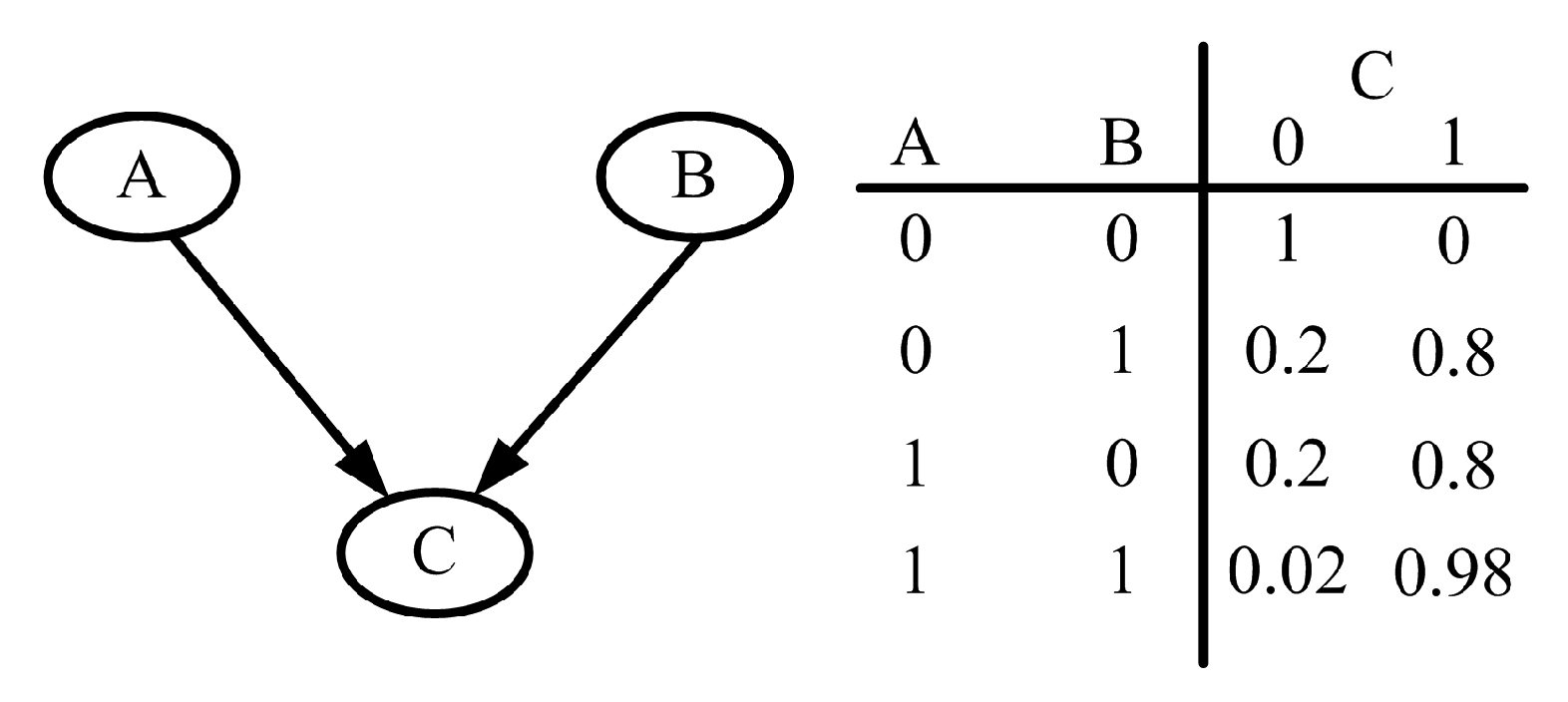
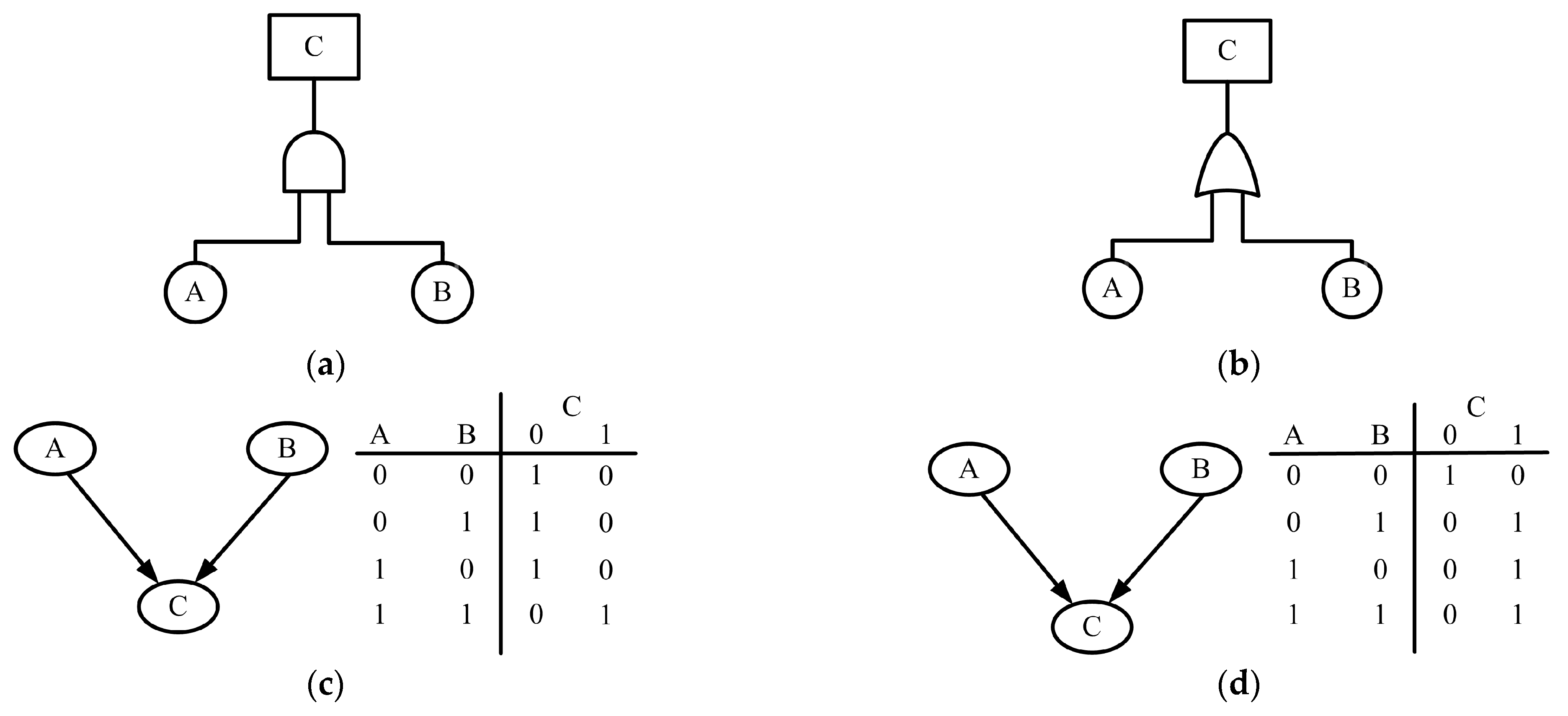
Traditional reliability analysis methods use deterministic expressions of two-state events to represent the logical relationships between events, and the results obtained from logical operations are also deterministic. Figure 2a,b shows the structure of a typical logic “AND” gate and logic “OR” gate in the FTA [36]. The “AND” gate shows top event C, and bottom events A and B appear at the same time. The “OR” gate shows that when bottom events A or B occur, top event C appears. The deterministic relationship between logic gates can be represented by Bayesian networks (Figure 2c,d).

In practical engineering applications, there are often uncertain logical relationships between events, and the logic gates of the FTA are no longer able to represent such uncertain logical relationships. However, Bayesian networks can solve this problem by the probability of manifestation of the uncertainties in the conditional probability table.

Similarly, the Bayesian network model corresponding to the “OR” gate in Figure 2d can be used to represent the logical relationship of uncertainty in terms of probability values (Figure 3).

As can be seen from Figure 3, output C must not occur only if neither input A nor B occur. When A and B occur at the same time, the probability of C occurring is 0.98, which is not necessarily occurring; when one of A and B occurs, C does not necessarily occur, so the interaction between input and output events A, B, and C is not a simple deterministic logic “AND” and logic “OR” but rather an uncertainty relationship between the two. Based on this, the uncertainty logical relationship between events is represented by Bayesian networks.

2.

Bayesian network models for polymorphic systems

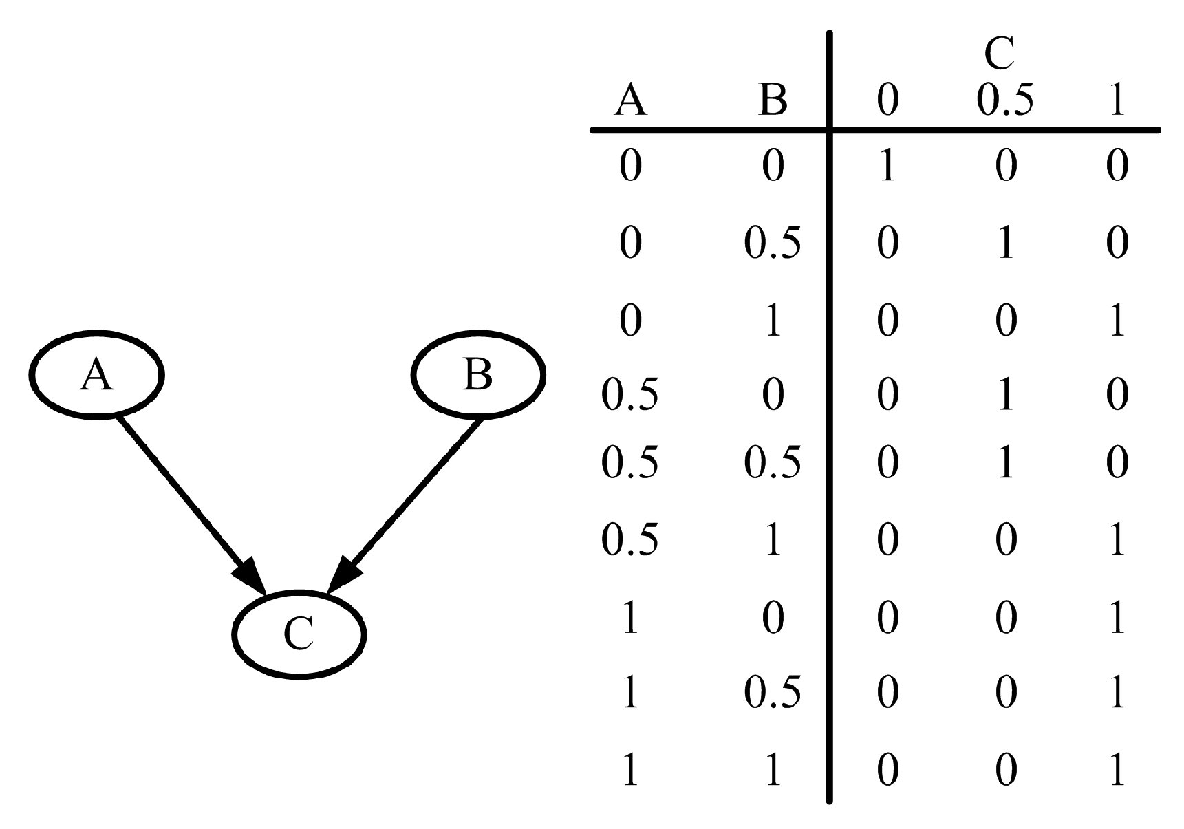
Bayesian networks can also be used to represent logical relationships between polymorphic systems. According to the definition of multi-state logic gates in Section 2.2, the values 0, 0.5, and 1 denote the normal, degradation, and failed states of the three-state system, respectively. According to Equation (6), the output event state is also normal with the normal input polymorphic events. When the input polymorphic events are in the degradation state or a combination of the degradation and normal states, the output event state is also in the degradation state. The whole system’s output fails when one input event fails. Figure 4 and Figure 5 represent the polymorphic logic gates under the FTA and Bayesian network models, respectively.

According to Figure 4, it can be seen that A and B are polymorphic input events with three states, 0, 0.5, and 1, and C is a polymorphic output event and also has three input states with the same state as the input event, and the polymorphic events A, B and C indicate the logical interaction among the three with polymorphic fault gates.

In comparison with Figure 4, in Figure 5, the polymorphic input events A and B are mapped to the polymorphic Bayesian network as root nodes, and the root nodes A and B also have three states. Output event C maps to a polymorphic Bayesian network as a leaf node of a polymorphic Bayesian network, and the polymorphic fault gate between polymorphic events A, B, and C maps to a polymorphic Bayesian network as a conditional probability table for a polymorphic Bayesian network. The one-way arrows of root nodes A and B pointing to C in Figure 5 indicate that root nodes A and B have an influential relationship on leaf node C, i.e., the leaf node’s state is affected by root nodes A and B.

2.4. Reliability Analysis Based on the BNs

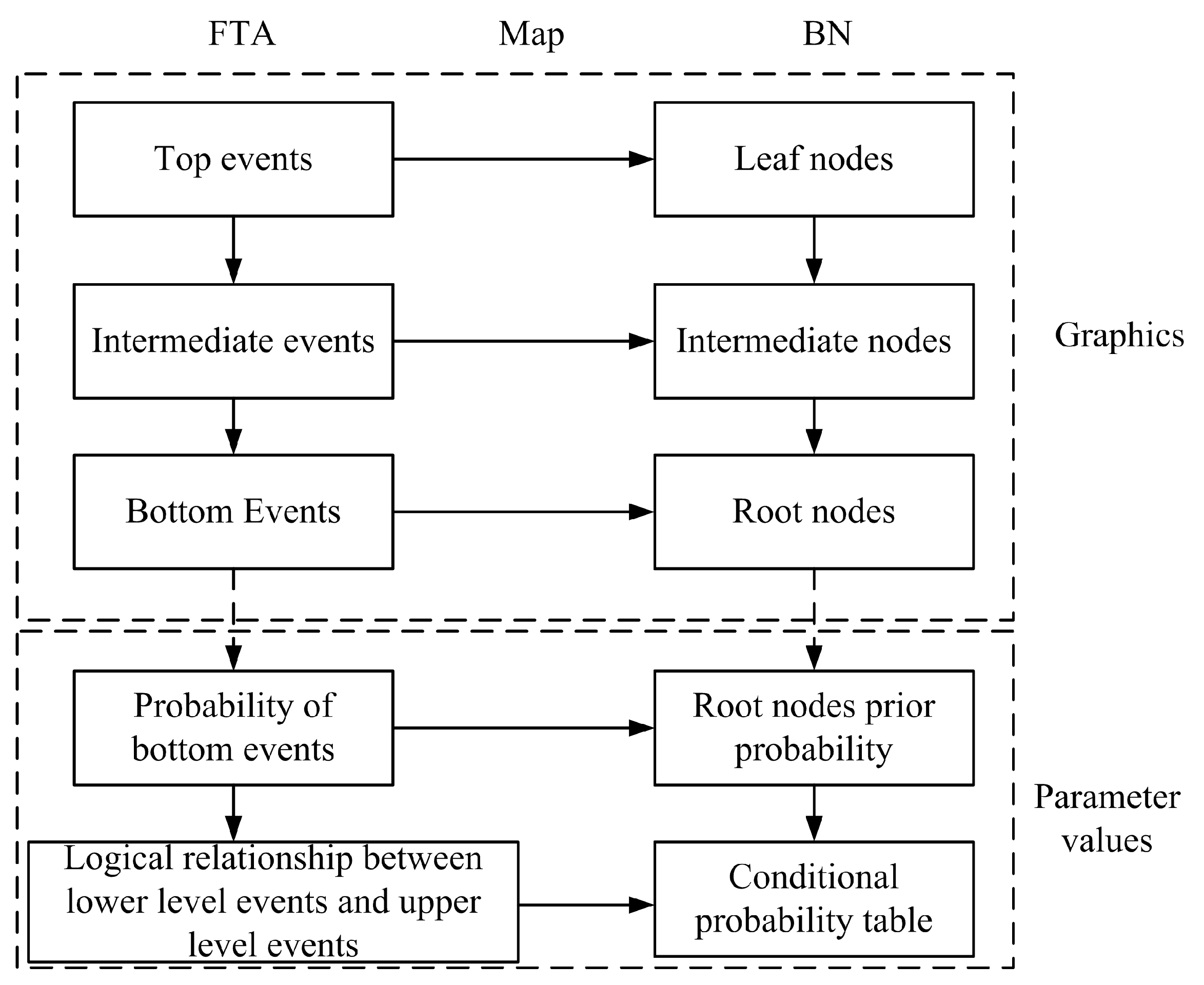
When using the Bayesian networks’ principle to analyze system reliability, the correspondence between the Bayesian networks and the FT is as follows: the basic events in the FT that cause the system to breakdown is used as the root node in the Bayesian networks, the intermediate node is the middle event of the FT, and the whole system failure event is used as the Bayesian network’s leaf node to build the Bayesian networks model. The logical block diagram for maps from the FTA to the BN according to the narrative is shown in Figure 6.

Assume that the BN model has $T, X_1,\dots ,X_{n-1}$ with a total of n nodes. $T$ denotes a leaf node, $X_1~X_{n-1}$ denote the root and intermediate nodes, respectively. The state of node T is denoted by $T_q$, and node $X_i(1\le i\le n-1)$’s actual state value is denoted by $x_i$. When the states $T_q$ and i take 0 or 1, this means that the event does not occurs or occurs, i.e., the normal state or the failure state. When the states $T_q$ and i take 0, 0.5, and 1, this signifies that the three-state event corresponds to the normal, degradation, and failure states. Using the junction probability distribution, the whole system’s failure probability is:

$$P\left(T=1\right)={\displaystyle \sum _{X_1,\dots ,X_{n-1}}P}\left(T=1,X_1=x_1,\dots ,X_{n-1}=x_{n-1}\right)$$

(13)

The posterior probability of other events occuring after event $X_j$ is:

$$P\left(X_i=1|X_j=1\right)=\frac{P\left(X_j=1|X_i=1\right)P\left(X_i=1\right)}{P\left(X_j=1\right)},\left(1\le i\ne j\le n-1\right)$$

(14)

Particularly, the posterior probability of node $X_i$’s occurrence is as follows with leaf node T occurrence:

$$P\left(X_i=1|T=1\right)=\frac{P\left(T=1|X_i=1\right)P\left(X_i=1\right)}{P\left(T=1\right)},\left(1\le i\le n-1\right)$$

(15)

The inference algorithm is used to solve bottom event $X_i$’s critical importance and probability importance.

• Probability importance

The basic event $X_i$ fault state being $x_i^a$’s probability importance $I_{T_q}^{Pr}(X_i=x_i^a)$ with respect to the top event T fault state being $T_q$ is:

$$I_{T_q}^{Pr}\left(X_i=x_i^a\right)=\left|P\left(T=T_q|X_i=x_i^a\right)-P\left(T=T_q|X_i=0\right)\right|$$

(16)

where $P\left(T=T_q|X_i=0\right)$ denotes the conditional probability that the T fault state is $T_q$ when the $X_i$ fault state is 0. The probability importance $I_{T_q}^{Pr}(X_i)$ of event $X_i$ with respect to the top event T fault state as $T_q$ is:

$$I_{T_q}^{Pr}\left(X_i\right)=\frac{1}{k_i-1}{\displaystyle \sum _{a_i=1}^{k_i}{I}_{T_q}^{Pr}\left(X_i=x_i^a\right)}$$

(17)

In Equation (17), $k_i$ is the number of fault states for event $X_i$.

2.

Critical importance

The basic event $X_i$ fault state being $x_i^a$’s critical importance $I_{T_q}^{Cr}(X_i=x_i^a)$ with respect to the top event T fault state being $T_q$ is:

$$I_{T_q}^{Cr}\left(X_i=x_i^a\right)=\frac{P\left(X_i=x_i^a\right)I_{T_q}^{Pr}\left(X_i=x_i^a\right)}{P\left(T=T_q\right)}$$

(18)

Then, the critical importance $I_{T_q}^{Cr}(X_i)$ of event $X_i$ with respect to the top event T fault state as $T_q$ is:

$$I_{T_q}^{Cr}\left(X_i\right)=\frac{1}{k_i-1}{\displaystyle \sum _{a_i=1}^{k_i}{I}_{T_q}^{Cr}\left(X_i=x_i^a\right)}$$

(19)

Probability importance indicates the change scope resulting from the occurrence of an event in the system. Critical importance reflects not only the change rate in probability resulting from that of an event occurring, but also the ease of improvement in the failure rate of that event [37]. The system failure’s key causes are identified by critical importance and probability importance.

3. Establishment of the Polymorphic Bayesian Network for the High-Voltage Drive Motor System

3.1. Establishment of the Polymorphic FT for the High-Voltage Drive Motor System

This manuscript takes the pure electric commercial vehicle L2 model of a vehicle manufacturer as the research object; the motor type chosen for the studied high-voltage drive motor system is a permanent magnet synchronous motor (PMSM), and its motor parameters are shown in

Table 2. Basic parameters of the PMSM.

Parameter	Rated Power	Maximum Power	Rated Speed	Maximum Speed	Rated Torque	Maximum Speed
Values	89 Kw	160 Kw	1700 r/min	4500 r/min	500 Nm	900 Nm

.

The complex operating conditions of pure electric commercial vehicles require drive motors that can adapt to frequent stopping, starting, accelerating, and decelerating. They also have the peculiarity of low/high torque at high/low speed; therefore, they require a high degree of reliability from the drive motor. The main causes of the functional degradation of drive motors are wear fault in the form of the presence of abrasive particles, excessive speed and high-temperature gluing. Plastic deformation can occur in the form of indentation, improper lubrication, etc. Corrosion failure can be caused by chemical corrosion, moisture, etc., and insulation deterioration can be caused by high-frequency pulse voltage, localized high temperatures, poor cooling, etc.

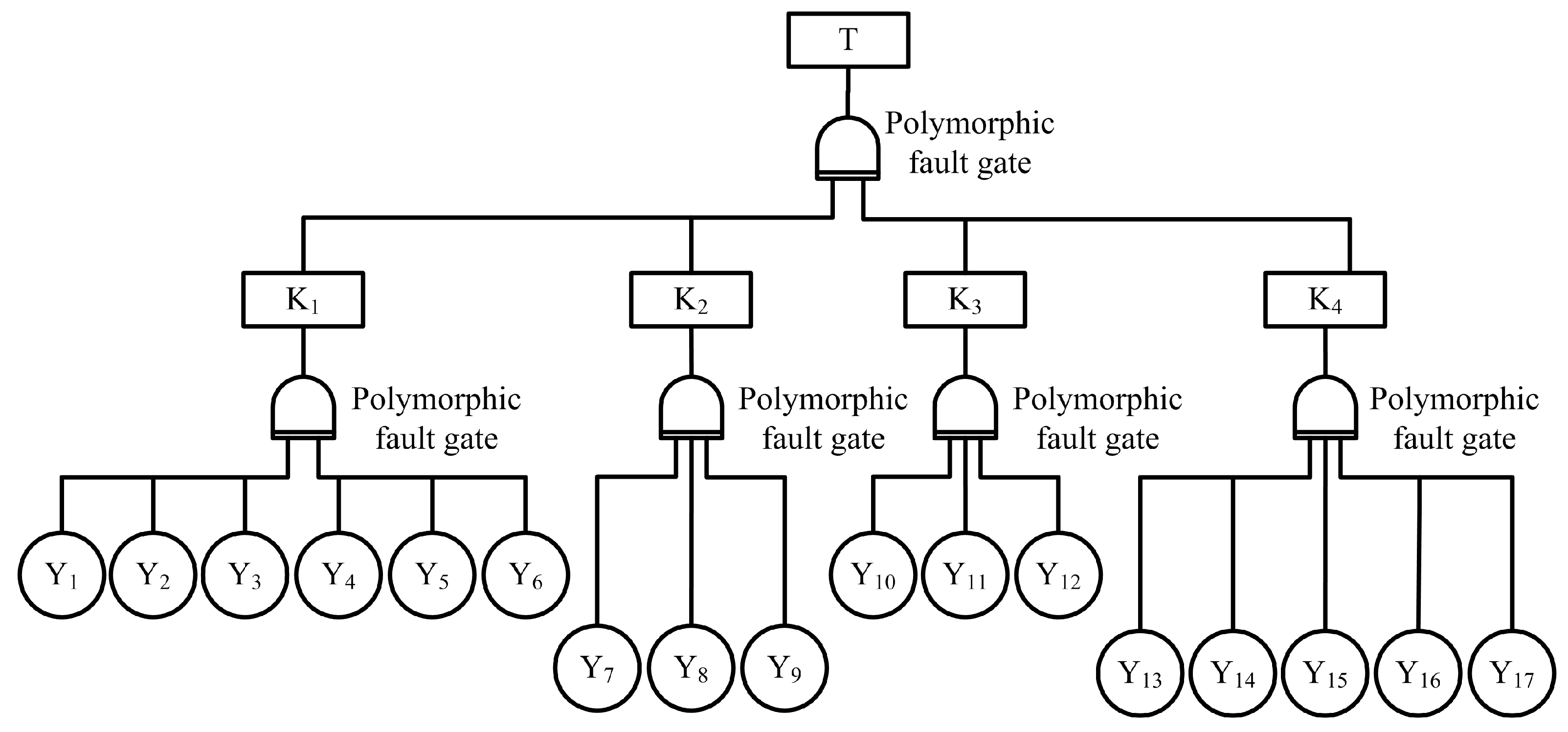
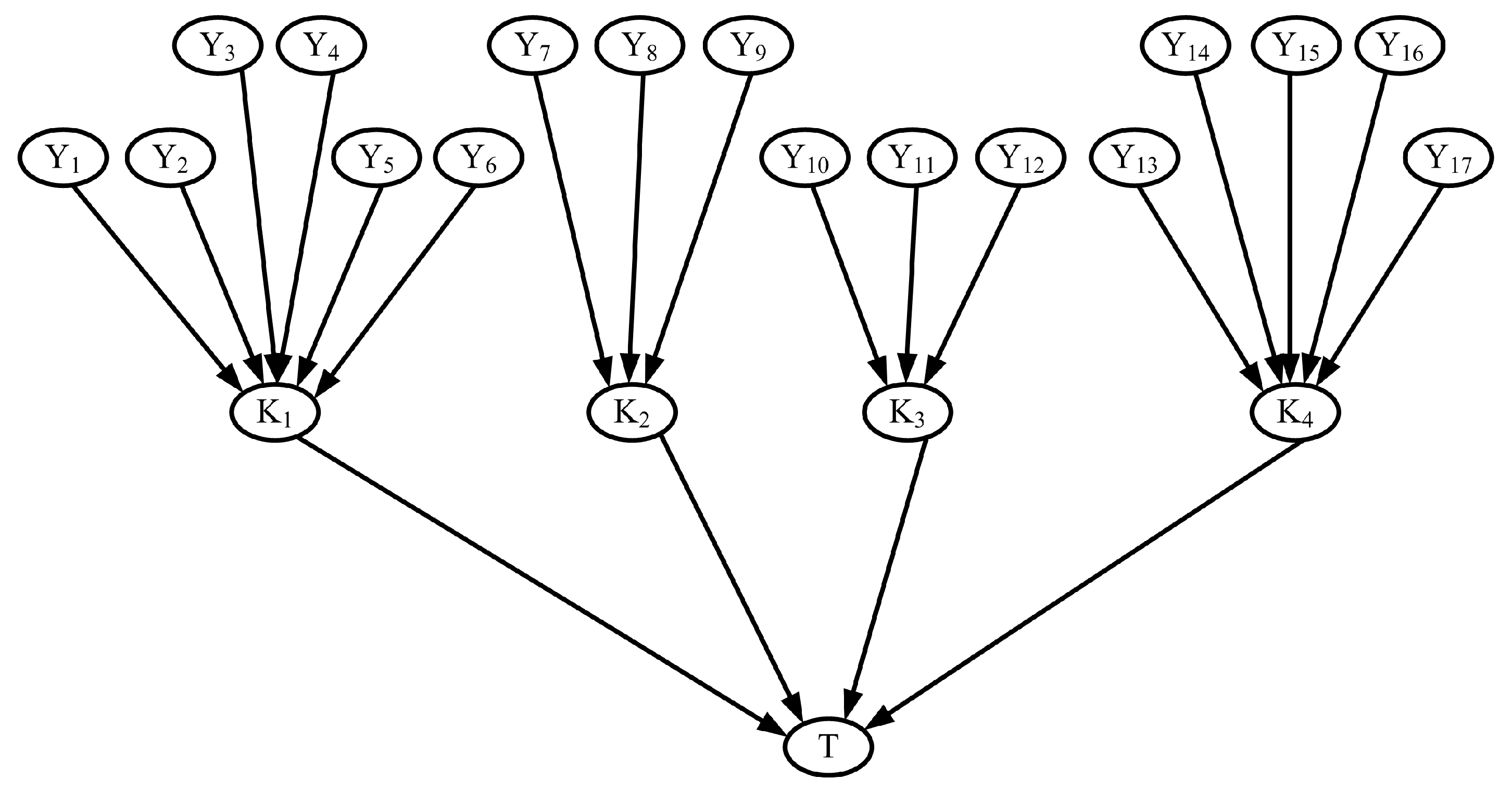
According to the cause of system degradation, the high voltage drive system degradation as the top event as well as the system failure event’s cause as the bottom event build a polymorphic fault tree and encode the events. The event definitions and codes are shown in

Table 3. Event codes and definitions.

Event	Code	Event	Code
System degradation	T	Wear fault	K1
Plastic deformation	K2	Corrosion failure	K3
Insulation deterioration	K4	Presence of abrasive particles	Y1
Excessive speed	Y2	Poor lubrication	Y3
Inappropriate clearance	Y4	High-temperature gluing	Y5
Scratch vibration	Y6	Indentation	Y7
Improper lubrication	Y8	Improper assembly	Y9
Moisture	Y10	Excessive inter-shaft current	Y11
Chemical corrosion	Y12	High-frequency pulse voltage	Y13
Localized high temperatures	Y14	Poor cooling	Y15
Severe partial discharges	Y16	Surface corrosion	Y17

—T is the failure of the pure electric commercial vehicle’s high-voltage power battery system. K₁, K₂, K₃, and K₄ are the intermediate events in the failure of a high-voltage drive motor system, where the occurrence of intermediate event K₁ can be caused by the occurrence of one of the bottom events Y₁, Y₂, Y₃, …, and Y₆. Similarly, the occurrence of K₂ is caused by one of Y₇, Y₈, and Y₉, and K₃ is caused by one of Y₁₀, Y₁₁, and Y₁₂, and the occurrence of any one of Y₁₃, Y₁₄, …, and Y₁₇ can lead to the occurrence of K₄.

Based on Table 3, the high-voltage drive motor system’s polymorphic FT of a purely electric commercial vehicle is simplified (Figure 7).

In Figure 7, Y₁, Y₂, …, and Y₁₇ are the polymorphic FT’s polymorphic bottom events, K₁, K₂, K₃, and K₄ are the intermediate events of the polymorphic FT, and T represents the polymorphic FT’s top event and the system failure’s top event.

3.2. Establishment of the Polymorphic Bayesian Network

When the conventional fault tree analysis method is used to analyse the reliability of a system, it can only analyze the probability of failure of the top event of the system in the two states of normal and failure of the bottom event represented by 0 and 1, i.e., the conventional fault tree analysis method can only be used to solve the reliability problem of a two-state system. However, bottom events such as surface corrosion and localized high temperatures in the high-voltage drive motor system cannot be accurately described by normal and failure states; they are polymorphic events that can be divided into normal, degradation and failure states, and the insulation deterioration caused by these two polymorphic bottom events is also a polymorphic event, i.e., it can be accurately described by normal, degradation, and failure states. Therefore, the conventional fault tree analysis method is not applicable to the analysis of the polymorphic system. In the polymorphic Bayesian network, the normal, degradation, and failure states of the polymorphic system are represented by 0, 0.5, and 1, respectively, which can more accurately analyze the reliability of the polymorphic system.

According to the high-voltage drive motor system’s polymorphic FT, the root node is the bottom event Y₁, Y₂, Y₃, …, and Y₁₇, the middle events K₁, K₂, K₃, and K₄ are the intermediate nodes, and the top event T is the leaf node to build the high-voltage drive motor system polymorphic Bayesian network model (Figure 8). In Figure 8, intermediate node K1 is a child of root nodes Y₁, Y₂, Y₃, Y₄, Y₅, and Y₆; intermediate node K₂ is a child of root nodes Y₇, Y₈, and Y₉; intermediate node K₃ is a child of root nodes Y₁₀, Y₁₁, and Y₁₂; intermediate node K₄ is a child of root nodes Y₁₃, Y₁₄, Y₁₅, Y₁₆, and Y₁₇; and leaf node T is a child of intermediate nodes K₁, K₂, K₃, and K₄. There are 17 root nodes, 4 middle nodes, and 1 leaf node.

In Figure 8, according to Equation (6) and Table 1, the input–output relationship between each polymorphic root node and intermediate node and between each intermediate node and leaf node can be obtained as follows: (1) there is a node with a state of 1 between the root nodes Y₁, Y₂, …, and Y₁₇, which will cause there to be a state of 1 in the intermediate nodes K₁, K₂, K₃, and K₄, that is, the leaf node has a state of 1. (2) When one of the root nodes Y₁, Y₂, …, and Y₁₇ has a state of 0.5, it will cause the intermediate nodes K₁, K₂, K₃, and K₄ to also have a node with a state of 0.5, which will eventually lead to a leaf node state of 0.5. (3) If and only if all root nodes have a state of 0, the intermediate node state is also 0, that is, the leaf node state is 0.

The CPT in Figure 8 can be deduced from Equation (6) and the CPT in the polymorphic logic gate under the Bayesian network model in Figure 5. Taking the conditional probability of node K₂ as an example, the CPT of the intermediate node K₂ and the root nodes Y₇, Y₈, and Y₉ is obtained as shown in

Table 4. Table of the conditional probabilities for the intermediate node K₂.

Y7	Y8	Y9	K2
			0	0.5	1
0	0	0	1	0	0
0	0	0.5	0	1	0
0	0	1	0	0	1
0	0.5	0	0	1	0
0	0.5	0.5	0	1	0
0	0.5	1	0	0	1
⋮	⋮	⋮	⋮	⋮	⋮
0	1	1	0	0	1
0.5	0	0	0	1	0
0.5	0	0.5	0	1	0
0.5	0	1	0	0	1
0.5	0.5	0	0	1	0
0.5	0.5	0.5	0	1	0
0.5	0.5	1	0	0	1
⋮	⋮	⋮	⋮	⋮	⋮
0.5	1	1	0	0	1
1	0	0	0	0	1
⋮	⋮	⋮	⋮	⋮	⋮
1	1	1	0	0	1

⋮—The case of the same conditional probability is omitted.

. The remaining CPTs between every root node, middle node, intermediate node, and leaf node can be deduced by referring to Equation (6) and Table 1, which are not detailed here.

4. Polymorphic Bayesian Network Model Solving

4.1. Calculation of the Occurrence Probability of the Top Event’s States

The prior probabilities of each root node in the polymorphic Bayesian network model of the high voltage drive motor system are shown in

Table 5. Each root node’s prior probability.

Root Node	States
	0	0.5	1
Y1	0.9973	0.001	0.0017
Y2	0.99952	0.0003	0.00018
Y3	0.9996	0.0002	0.0002
Y4	0.99965	0.00025	0.0001
Y5	0.9973	0.001	0.0017
Y6	0.99952	0.0003	0.00018
Y7	0.9997	0.0002	0.0001
Y8	0.9996	0.0002	0.0002
Y9	0.99965	0.00025	0.0001
Y10	0.9973	0.001	0.0017
Y11	0.99952	0.0003	0.00018
Y12	0.99965	0.00025	0.0001
Y13	0.9996	0.0002	0.0002
Y14	0.9973	0.001	0.0017
Y15	0.99952	0.0003	0.00018
Y16	0.9996	0.0002	0.0002
Y17	0.99965	0.00025	0.0001

.

Based on Figure 8, a simulation model of the polymorphic Bayesian network was built in GenIe simulation software, and the model includes the conditional probabilities in Table 3 and the prior probabilities of each root node in Table 4. Inference on the polymorphic Bayesian network models is provided by GenIe and Equation (13). The top event T failure probability is gained:

$$\begin{array}{l}P\left(T=1\right)={\displaystyle \sum _{\begin{array}{l}{Y}_1,Y_2,\dots Y_{17}\\ K_1,\dots K_4\end{array}}P\left(Y_1,Y_2,\dots ,Y_{17},K_1,\dots ,K_4,T=1\right)}={\displaystyle \sum _{K_1,\dots ,K_4}P\left(T=1|K_1,\dots ,K_4\right)}\times {\displaystyle \sum _{Y_1,\dots ,Y_6}P\left(K_1|Y_1,\dots ,Y_6\right)}\times P\left(Y_1\right)\dots P\left(Y_6\right)\\ \times {\displaystyle \sum _{Y_7,Y_8,Y_9}P\left(K_2|Y_7,Y_8,Y_9\right)\times P\left(Y_7\right)}\times P\left(Y_8\right)\times P\left(Y_9\right)\times \dots \times {\displaystyle \sum _{Y_{13},\dots ,Y_{17}}P\left(K_4|Y_{13},\dots ,Y_{17}\right)\times P\left(Y_{13}\right)\times \dots P\left(Y_{17}\right)}\end{array}$$

(20)

Using the conditional probability between the nodes in Table 1 and the a priori probability of each root node, the top event’s failure probability is obtained as:

$$P\left(T=1\right)=0.00878$$

Similarly, the top event’s probabilities in the normal and degradation states are:

$$\begin{gathered} P\left(T=0\right)=0.9841 \\ P\left(T=0.5\right)=0.00712 \end{gathered}$$

According to the relationship between the reliability and the failure rate of the system in Equation (4), the system’s reliability is:

$$R_T=0.9913$$

Based on the interaction between the unreliability and the reliability of Equation (5), system’s unreliability is:

$$F_T=1-R_T=0.0087$$

4.2. Solution of the Basic Event’s Posterior Probability

The failure state’s posterior probability Y₁ of the bottom event with the top event T as the failure state is derived from Equation (15) as:

$$P\left(Y_1=1|T=1\right)=\frac{P\left(T=1|Y_1=1\right)P\left(Y_1=1\right)}{P\left(T=1\right)}=0.1935$$

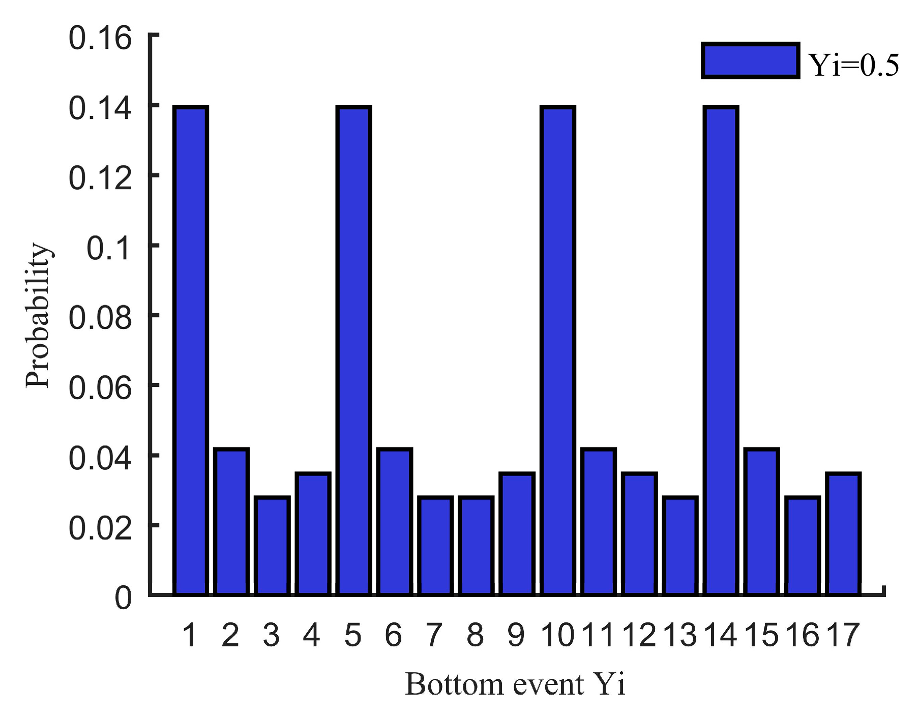
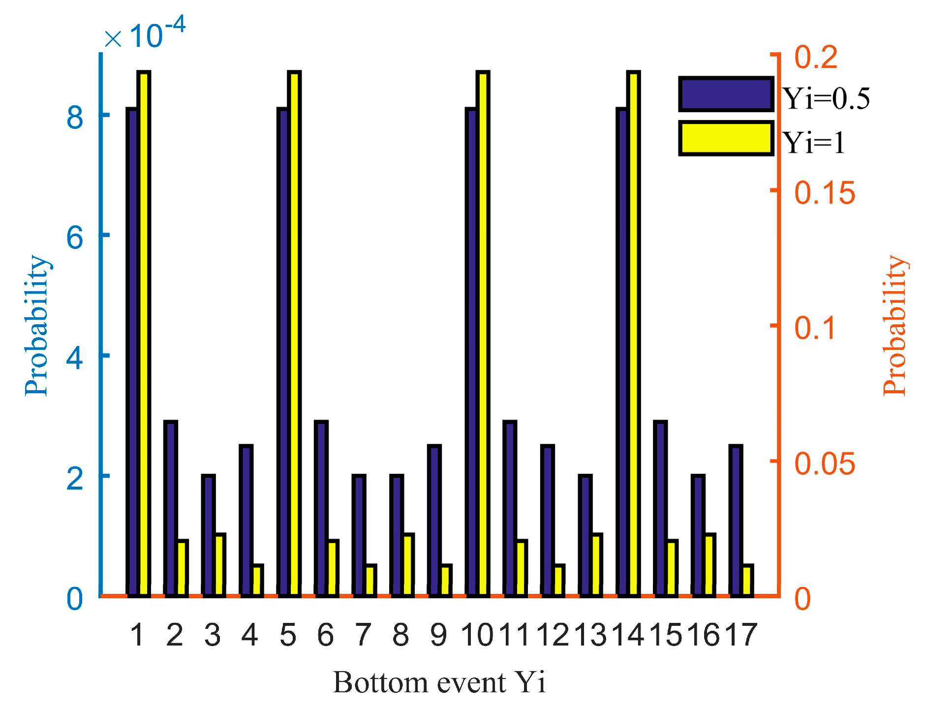
Similarly, the posterior probabilities of the bottom event $Y_i(i=0,\dots ,17)$ state of 0.5 or 1 can be obtained under the condition that the top event T is 0.5 or 1. According to Table 5, the leaf node is in state 1 when the state of at least one root node is in state 1, that is, the bottom event’s posterior probability $Y_i$ in state 1 is 0 when the top event T is in state of 0.5. The posterior probabilities of the events at the bottom as indicated in

Table 6. Posterior probabilities of the bottom event.

Root Node	Posterior Probabilities
	$\mathit{P}({\mathit{Y}}_{\mathit{i}}=0.5|\mathit{T}=0.5)$	$\mathit{P}({\mathit{Y}}_{\mathit{i}}=0.5|\mathit{T}=1)$	$\mathit{P}({\mathit{Y}}_{\mathit{i}}=1|\mathit{T}=1)$
Y1	0.13944	0.00081	0.19346
Y2	0.04177	0.00029	0.02048
Y3	0.02785	0.00020	0.02276
Y4	0.03480	0.00025	0.01138
Y5	0.13944	0.00081	0.19346
Y6	0.04177	0.00029	0.02048
Y7	0.02784	0.00020	0.01138
Y8	0.02785	0.00020	0.02276
Y9	0.03480	0.00025	0.01138
Y10	0.13944	0.00081	0.19346
Y11	0.04177	0.00029	0.02048
Y12	0.03480	0.00025	0.01138
Y13	0.02785	0.00020	0.02276
Y14	0.13944	0.00081	0.19346
Y15	0.04177	0.00029	0.02048
Y16	0.02785	0.00020	0.02276
Y17	0.03480	0.00025	0.01138

.

According to the conditional probability table in Table 5, when the parent node is in state of 0.5, the child node state 1 of probability is 0, that is, when T is 0.5, the root node Y_i’s posterior probability is 0. To more intuitively describe the comparative relationship between the posterior probabilities of every basic event, a comparative histogram of the posterior probabilities of each floor event was plotted from Table 6 as shown in Figure 9 and Figure 10.

The system can be anatomized by the bottom’s posterior failure probability after the fault of the system, that is, the judgement is found out in the sequence of each bottom event’s posterior probability from largest to smallest. According to Figure 9, once system functional degradation has been observed, a fault analysis should be performed on the bottom events in a degraded state in the order: Y₁, Y₅, Y₁₀, Y₁₄, …, Y₁₆, and Y₇. According to Figure 10, once system functional failure has been observed, a fault analysis should be performed on the basic events in a degraded state in the order: Y₁, Y₅, Y₁₀, Y₁₄, …, and Y₁₆, Y₇, and a fault analysis should be performed on the floor events in the failure state in the sequence: Y₁, Y₅, Y₁₀, Y₁₄, …, Y₁₇, and Y₇.

4.3. Solution to the Basic Event Importance

• Probability importance

The bottom event’s probability importance Y₁ being in the degradation state of 0.5 with respect to the top event T being in the degradation state of 0.5 is derived from Equation (16) as:

$$I_{0.5}^{Pr}\left(Y_1=0.5\right)=\left|P\left(T=0.5|Y_1=0.5\right)-P\left(T=0.5|Y_1=0\right)\right|=0.9868$$

The probability importance that the base event Y₁ is in failed state 1 and is in a degenerate state relative to the top event T being in the state of 0.5 is:

$$I_{0.5}^{Pr}\left(Y_1=1\right)=\left|P\left(T=0.5|Y_1=1\right)-P\left(T=0.5|Y_1=0\right)\right|=0.00614$$

The basis event’s probability importance Y₁ related to the upper layer event T being in the fault state of 0.5 is derived from Equation (17) as:

$$I_{0.5}^{Pr}\left(Y_1\right)=\frac{\left[I_{0.5}^{Pr}\left(Y_1=0.5\right)+I_{0.5}^{Pr}\left(Y_1=1\right)\right]}{2}=0.49647$$

Similarly, the probability importance that the underlying event Y₁ is in the failed state of 0.5 relative to the top-level event T being in the failed state 1 is:

$$I_1^{Pr}\left(Y_1=0.5\right)=\left|P\left(T=1|Y_1=0.5\right)-P\left(T=1|Y_1=0\right)\right|=0$$

The probability importance that the bottom event Y₁ is in the fault state 1 relative to the top event T being in the fault state 1 is:

$$I_1^{Pr}\left(Y_1=1\right)=\left|P\left(T=1|Y_1=1\right)-P\left(T=1|Y_1=0\right)\right|=0.9929$$

The floor event’s probability importance Y₁ related to the upper layer event T being in the fault state 1 is derived from Equation (17) as:

$$I_1^{Pr}\left(Y_1\right)=\frac{\left[I_1^{Pr}\left(Y_1=0.5\right)+I_1^{Pr}\left(Y_1=1\right)\right]}{2}=0.49645$$

Similarly, the floor event’s probability importance Y_i related to the upper layer event T being in the fault states 0.5 and 1 is derived from Equations (16) and 17, as pointed out in

Table 7. The bottom event’s probability importance Y_i with respect to the upper layer event T being in the fault states 0.5 and 1.

$\mathbf{Root} \mathbf{Node} {\mathit{Y}}_{\mathit{i}}$	${\mathit{I}}_{0.5}^{\mathit{P}\mathit{r}}\left({\mathit{Y}}_{\mathit{i}}\right)$	${\mathit{I}}_1^{\mathit{P}\mathit{r}}\left({\mathit{Y}}_{\mathit{i}}\right)$
Y1	0.49647	0.49645
Y2	0.49572	0.49570
Y3	0.49572	0.49571
Y4	0.49564	0.49566
Y5	0.49647	0.49645
Y6	0.49572	0.49570
Y7	0.49566	0.49566
Y8	0.49572	0.49571
Y9	0.49564	0.49566
Y10	0.49647	0.49645
Y11	0.49572	0.49570
Y12	0.49564	0.49566
Y13	0.49572	0.49571
Y14	0.49647	0.49645
Y15	0.49572	0.49570
Y16	0.49572	0.49571
Y17	0.49564	0.49566

.

The probability importance line chart was drawn according to Table 7 (Figure 11).

2.

Critical importance

The critical importance of the bottom event Y₁ being in the breakdown state of 0.5 with respect to the top event T being in the breakdown state of 0.5 is derived from Equation (18) as:

$$I_{0.5}^{Cr}\left(Y_1=0.5\right)=\frac{P\left(Y_1=0.5\right)I_{0.5}^{Pr}\left(Y_1=0.5\right)}{P\left(T=0.5\right)}=0.13860$$

The critical importance of the floor event Y₁ being in the failure state of 1 with respect to the top event T being in the breakdown state of 0.5 is:

$$I_{0.5}^{Cr}\left(Y_1=1\right)=\frac{P\left(Y_1=1\right)I_{0.5}^{Pr}\left(Y_1=1\right)}{P\left(T=0.5\right)}=0.001466$$

The critical importance of the floor event Y₁ with respect to the upper layer event T being in the fault state of 0.5 is derived from Equation (19) is:

$$I_{0.5}^{Cr}\left(Y_1\right)=\frac{\left[I_{0.5}^{Cr}\left(Y_1=0.5\right)+I_{0.5}^{Cr}\left(Y_1=1\right)\right]}{2}=0.07003$$

Similarly, the critical importance of the floor event Y₁ being in the fault state of 0.5 related to the top event T being in the breakdown state of 1 is:

$$I_1^{Cr}\left(Y_1=0.5\right)=\frac{P\left(Y_1=0.5\right)I_1^{Pr}\left(Y_1=0.5\right)}{P\left(T=1\right)}=0$$

The critical importance of the floor event Y₁ being in the fault state of 1 with respect to the upper layer event T being in the fault state of 1 is:

$$I_1^{Cr}\left(Y_1=1\right)=\frac{P\left(Y_1=1\right)I_1^{Pr}\left(Y_1=1\right)}{P\left(T=1\right)}=0.19225$$

The critical importance of the floor event Y₁ with respect to the upper layer event T being in fault state of 1 is derived from Equation (19) is:

$$I_1^{Cr}\left(Y_1\right)=\frac{\left[I_1^{Cr}\left(Y_1=0.5\right)+I_1^{Cr}\left(Y_1=1\right)\right]}{2}=0.09612$$

Similarly, the critical importance of the floor event Y_i with respect to the upper layer event T being in the fault states of 0.5 and 1 is derived from Equations (18) and (19), as shown in

Table 8. The bottom event’s critical importance Y_i related to the top event T being in the fault states of 0.5 and 1.

$\mathbf{Root} \mathbf{Node} {\mathit{Y}}_{\mathit{i}}$	${\mathit{I}}_{0.5}^{\mathit{C}\mathit{r}}\left({\mathit{Y}}_{\mathit{i}}\right)$	${\mathit{I}}_1^{\mathit{C}\mathit{r}}\left({\mathit{Y}}_{\mathit{i}}\right)$
Y1	0.07003	0.09612
Y2	0.02083	0.01016
Y3	0.01392	0.01129
Y4	0.01733	0.00565
Y5	0.07003	0.09612
Y6	0.02083	0.01016
Y7	0.01387	0.00565
Y8	0.01392	0.01129
Y9	0.01733	0.00565
Y10	0.07033	0.09612
Y11	0.02083	0.01016
Y12	0.01733	0.00565
Y13	0.01392	0.01129
Y14	0.07003	0.09612
Y15	0.02083	0.01016
Y16	0.01392	0.01129
Y17	0.01733	0.00565

.

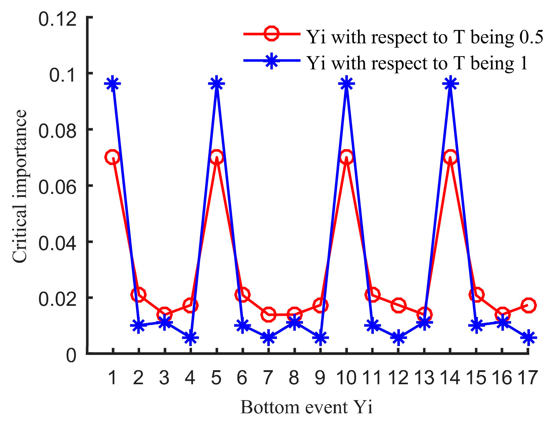
The critical importance line chart shown in Figure 12 was drawn according to the results in Table 8.

4.4. System Reliability Analysis

Based on each error mode’s critical importance and probability importance for the different failure states of the system, it can be shown how much each failure state affects the system and vulnerable points in the system can be confirmed. It can be seen from Figure 11 that the order of the impact extent of the root node Y_i on the system’s breakdown state in the degradation state is: $Y_1=Y_5=Y_{10}=Y_{14}>Y_3>\dots >Y_{17}$. The order of the root node’s impact extent Y_i on the system’s error state in the failure state is: $Y_1=Y_5=Y_{10}=Y_{14}>Y_3>\dots >Y_{17}$. Similarly, as can be seen from the critical importance curve of the basic event with regards to the top-level event fault state in Figure 12, the order of the root node’s impact extent Y_i on the system’s breakdown state in the degradation state is: $Y_1=Y_5=Y_{10}=Y_{14}>Y_2>\dots >Y_7$. The order of the root node’s impact extent Y_i on the system’s breakdown state in the failure state is: $Y_1=Y_5=Y_{10}=Y_{14}>Y_2>\dots >Y_{17}$.

In summary, according to the conclusions of the floor event’s probability importance to the system in different fault states, it can be seen that the breakdown states of the bottom events Y₁, Y₅, Y₁₀, and Y₁₄ have the biggest impact on the system’s fault state, and according to the conclusions of the bottom event’s critical importance to the system in different breakdown states, it can be seen that the bottom events Y₁, Y₅, Y₁₀, and Y₁₄ as the weak link of the polymorphic system are more difficult to improve, that is, they are the weakest link of the system, and the corresponding bottom events are: the presence of abrasive particles, high-temperature gluing, moisture, and localized high temperatures. The analysis shows that the bottom events Y₁, Y₅, Y₁₀, and Y₁₄ require special attention and improvement to reduce the occurrence of serious failures.

Meanwhile, according to each root node’s posterior probabilities in the previous sections, it can be seen that after the system’s degradation or failure fault, the root nodes causing the highest fault occurrence probability are Y₁, Y₅, Y₁₀, and Y₁₄, i.e., the presence of abrasive particles, high-temperature gluing, moisture, and localized high temperatures. When carrying out detection and fault diagnosis in a pure electric commercial vehicle’s high-voltage drive motor system, whole system detection is enhanced by selecting the bottom event with a high posterior probability according to each basic event’s occurrence in the high-voltage drive motor system.

When optimizing the reliability of the system, improvements should be made in the following two areas in case of system wear failure due to the presence of abrasive particles: (1) enhanced lubrication. Filling the frequent friction surface with lubricating oil greatly reduces the friction coefficient, thus contributing to a reduction in frictional resistance and a reduction in mechanical wear. (2) Improve the quality of installation and maintenance. Correctly tightening the motor bearing cover and the bearing seat connection screws, so that the combination of the face is in the center, and adjusting the appropriate bearing clearance, etc., can make the unit load on the surface of the uniform distribution so that its wear is reduced. The system should be improved in the following three ways in case of corrosion failure due to moisture: (1) adopt a sealed design to prevent moisture from entering the motor interior. Clean and dry the inside of the motor casing before sealing and reduce the humidity inside the sealed cavity as much as possible to avoid condensation inside at low temperatures. (2) For large mechanical mechanisms such as motors, design ventilation holes, moisture-proof mats, and other measures to eliminate moisture. (3) Adjust the humidity inside the cavity by adding moisture-regulating plates, moisture absorbers, etc.

Therefore, the bottom event—the presence of abrasive particles, high-temperature gluing, moisture, and localized high temperatures—is the most important and the weakest link in the high-voltage drive motor system, and the above measures can be taken to improve the reliability of the system.

5. Conclusions

The reliability of the high-voltage drive motor system was analyzed by taking a pure electric commercial vehicle as the research object, dividing the system and its bottom event into three states of normal, degradation, and failure, and determining the probability of the top event of the system in the normal state, the degradation state, and the failure state as 0.9841, 0.00712, and 0.00878, respectively, and solving the reliability of the high-voltage drive motor system as 0.9913.

In this paper, based on the traditional fault tree analysis method, we mainly accomplish the following: (1) combining the fault tree analysis method with the basic theory of polymorphic Bayesian networks, establishing the polymorphic fault tree of a high-voltage drive motor system, transforming the polymorphic fault tree into a polymorphic Bayesian network model according to the maps relationship between the fault tree and the Bayesian network, and solving the occurrence probability of leaf nodes in each state by Bayesian network inference, and the posterior probability of the occurrence of the polymorphic bottom event when the top event was in different fault states was solved. The posterior probability of the polymorphic bottom event was analyzed to find out the most likely event after system failure. (2) The quantitative analysis of the polymorphic root node was analyzed from the perspective of probability importance and critical importance to find out that the presence of abrasive particles, high-temperature gluing, moisture, and localized high temperatures are the weakest link in the high-voltage drive motor system and the most difficult bottom event to improve and optimize the system.

Finally, the detection and design optimization of the system based on the probability importance degree and the critical importance degree of the bottom event can improve the efficiency of subsequent fault diagnosis, which is of great significance for improving the high voltage drive motor system of pure electric commercial vehicles.

References

1. Huang, H.-Z.; Tong, X.; Zuo, M.J. Posbist fault tree analysis of coherent systems. Reliab. Eng. Syst. Saf. 2004, 84, 141–148. [Google Scholar] [CrossRef]
2. Dhillon, B.S. Design Reliability: Fundamentals and Applications, 1st ed.; CRC Press: Boca Raton, FL, USA; London, UK; New York, NY, USA; Washington, DC, USA, 1999; pp. 167–182. [Google Scholar]
3. Cao, C.; Li, M.; Li, Y.; Sun, Y. Intelligent fault diagnosis of hot die forging press based on binary decision diagram and fault tree analysis. Procedia Manuf. 2018, 15, 459–466. [Google Scholar] [CrossRef]
4. Li, Y.; Song, X.; Zhao, S.; Gao, F. A Line-Fault Cause Analysis Method for Distribution Network Based on Decision-Making Tree and Machine Learning. In Proceedings of the 2020 5th Asia Conference on Power and Electrical Engineering (ACPEE), Chengdu, China, 4–7 June 2020. [Google Scholar] [CrossRef]
5. Jiao, M.; Huang, Y.; Shi, J.; Cai, F.; Lin, R. Fault Diagnosis of Simplified Fault Trees using State Transition Diagrams. In Proceedings of the 2020 27th Asia-Pacific Software Engineering Conference (APSEC), Singapore, 1–4 December 2020. [Google Scholar] [CrossRef]
6. Waghen, K.; Ouali, M.-S. Multi-level interpretable logic tree analysis: A data-driven approach for hierarchical causality analysis. Expert Syst. Appl. 2021, 178, 115035. [Google Scholar] [CrossRef]
7. Tanaka, H.; Fan, L.T.; Lai, F.S.; Toguchi, K. Fault-Tree Analysis by Fuzzy Probability. IEEE Trans. Reliab. 1983, R-32, 453–457. [Google Scholar] [CrossRef]
8. Shi, S.; Jiang, B.; Meng, X.; Yang, L. Fuzzy fault tree analysis for gas explosion of coal mining and heading faces in underground coal mines. Adv. Mech. Eng. 2018, 10, 1687814018792318. [Google Scholar] [CrossRef]
9. Nadjafi, M.; Farsi, M.; Khamnei, H.J. Quantitative based fault tree analysis: An integrated fuzzy Monte Carlo and its application on launch escape emergency detection system. J. Intell. Fuzzy Syst. 2018, 35, 845–859. [Google Scholar] [CrossRef]
10. Cui, T.-J.; Li, S.-S. Study on the construction and application of discrete space fault tree modified by fuzzy structured element. Clust. Comput. 2019, 22, 6563–6577. [Google Scholar] [CrossRef]
11. Li, L.; Liang, Q.; Liang, Y. Fuzzy Fault Tree Analysis of a Gas Turbine Fuel System. IOP Conf. Series Earth Environ. Sci. 2019, 237, 022024. [Google Scholar] [CrossRef]
12. Jianxing, Y.; Haicheng, C.; Yang, Y.; Zhenglong, Y. A weakest t-norm based fuzzy fault tree approach for leakage risk assessment of submarine pipeline. J. Loss Prev. Process. Ind. 2019, 62, 103968. [Google Scholar] [CrossRef]
13. Cowell, R.G.; Dawid, A.P.; Lauritzen, S.L.; Spiegelhalter, D.J. Probabilistic Networks and Expert Systems; Springer: New York, NY, USA, 1999; pp. 14–21. [Google Scholar]
14. Portinale, L.; Bobbio, A. Bayesian networks for dependability analysis: An application to digital control reliability. In Proceedings of the 15th Conference on Uncertainty in Artificial Intelligence, Stockholm, Sweden, 30 July–1 August 1999; pp. 551–558. [Google Scholar]
15. Mahadevan, S.; Zhang, R.; Smith, N. Bayesian networks for system reliability reassessment. Struct. Saf. 2001, 23, 231–251. [Google Scholar] [CrossRef]
16. Liu, Y.; Zhang, Z.; Zhong, M. Reliability analysis on the injection system by mapping t-s fault trees into bayesian networks. In Proceedings of the 3rd International Conference on Mechatronics, Robotics and Automation (ICMRA 2015), Shenzhen, China, 20–21 April 2015; pp. 1134–1139. [Google Scholar]
17. Wang, H.; Duan, F.; Ma, J. Reliability analysis of complex uncertainty multi-state system based on Bayesian network. Eksploat. i Niezawodn. Maint. Reliab. 2019, 21, 419–429. [Google Scholar] [CrossRef]
18. Feng, X.; Jiang, J.-C.; Feng, Y.-G. Reliability evaluation of gantry cranes based on fault tree analysis and Bayesian network. J. Intell. Fuzzy Syst. 2020, 38, 3129–3139. [Google Scholar] [CrossRef]
19. Guo, Y.; Zhong, M.; Gao, C.; Wang, H.; Liang, X.; Yi, H. A discrete-time bayesian network approach for reliability analysis of dy-namic systems with common cause failures. Reliab. Eng. Syst. Saf. 2021, 216, 108028. [Google Scholar] [CrossRef]
20. Li, H.; Soares, C.G.; Huang, H.-Z. Reliability analysis of a floating offshore wind turbine using Bayesian Networks. Ocean Eng. 2020, 217, 107827. [Google Scholar] [CrossRef]
21. Mao, K.; Liu, X.; Li, S.; Wang, X. Reliability analysis for mechanical parts considering hidden cost via the modified quality loss model. Qual. Reliab. Eng. Int. 2021, 37, 1373–1395. [Google Scholar] [CrossRef]
22. Wang, Y.; Liu, X.; Wang, H.; Wang, X.; Wang, X. Improved fatigue failure model for reliability analysis of mechanical parts inducing stress spectrum. Proc. Inst. Mech. Eng. Part O J. Risk Reliab. 2021, 235, 973–981. [Google Scholar] [CrossRef]
23. Teng, D.; Feng, Y.-W.; Chen, J.-Y.; Lu, C. Structural dynamic reliability analysis: Review and prospects. Int. J. Struct. Integr. 2022, 13, 753–783. [Google Scholar] [CrossRef]
24. Lu, S.; Shi, D.; Xiao, H. Reliability of sliding window systems with two failure modes. Reliab. Eng. Syst. Saf. 2019, 188, 366–376. [Google Scholar] [CrossRef]
25. Zhang, Y.R.; Liu, X.T.; Geng, S.L. Reliability analysis and evaluation of wheel axle for high-speed train considering interference fit. J. Chin. Soc. Mech. Eng. 2022, 43, 265–274. [Google Scholar]
26. Yazdi, M.; Zarei, E.; Adumene, S.; Abbassi, R.; Rahnamayiezekavat, P. Chapter eleven—uncertainty modeling in risk assessment of digitalized process systems. In Methods in Chemical Process Safety; Khan, F., Pasman, H., Yang, M., Eds.; Elsevier: Amsterdam, The Netherlands, 2022; pp. 389–416. [Google Scholar]
27. Yazdi, M.; Adumene, S.; Zarei, E. Introducing a Probabilistic-Based Hybrid Model (Fuzzy-BWM-Bayesian Network) to Assess the Quality Index of a Medical Service. In Linguistic Methods Under Fuzzy Information in System Safety and Reliability Analysis; Yazdi, M., Ed.; Springer International Publishing: Cham, Switzerland, 2022; pp. 171–183. [Google Scholar] [CrossRef]
28. O’Connor, P.; Kleyner, A. Practical Reliability Engineering, 5th ed.; John Wiley & Sons, Ltd.: Chichester, UK, 2012; pp. 19–69. [Google Scholar]
29. Jiang, H.; Lin, C.; Feng, G.; Xu, E.; Zheng, W. Reliability Analysis of the High-Voltage Power Battery System Based on the Polymorphic Fuzzy Fault Tree. J. Sensors 2022, 2022, 2455345. [Google Scholar] [CrossRef]
30. Li, X.; Tang, W. Structural risk analysis model of damaged membrane LNG carriers after grounding based on Bayesian belief networks. Ocean Eng. 2019, 171, 332–344. [Google Scholar] [CrossRef]
31. Boudali, H.; Dugan, J.B. A new bayesian network approach to solve dynamic fault trees. In Proceedings of the 51st Annual Reliability and Maintain-ability Symposium (RAMS), Alexandria, VA, USA, 24–27 January 2005; pp. 451–456. [Google Scholar]
32. Zhang, R.J.; Zhang, L.L.; Dong, M.X. Multi-state system importance analysis method of fuzzy bayesian networks. Int. J. Ind. Syst. Eng. 2015, 21, 395–414. [Google Scholar] [CrossRef]
33. Mi, J.; Li, Y.; Huang, H.-Z.; Liu, Y.; Zhang, X. Reliability analysis of multi-state systems with common cause failure based on Bayesian Networks. Eksploat. Niezawodn. 2013, 15, 169–175. [Google Scholar] [CrossRef]
34. Chen, D.; Fan, Y.; Ye, C.; Zhang, S. Human reliability analysis for manned submersible diving process based on CREAM and Bayesian network. Qual. Reliab. Eng. Int. 2019, 35, 2261–2277. [Google Scholar] [CrossRef]
35. Sun, Y.; Chen, K.; Liu, C.; Zhang, Q.; Qin, X. Research on reliability analytical method of complex system based on CBN model. J. Mech. Sci. Technol. 2021, 35, 107–120. [Google Scholar] [CrossRef]
36. Chen, H.; Dong, F.; Xu, S.; Yang, J.; Chan, C.C. Reliability Evaluation of Switched Reluctance Motor Drive System in Electric Vehicle Based on Bayesian Network. In Proceedings of the 2019 IEEE Vehicle Power and Propulsion Conference (VPPC), 16th IEEE Vehicle Power and Propulsion Conference (VPPC), Hanoi, Vietnam, 14–17 October 2019. [Google Scholar] [CrossRef]
37. Guan, F.; Zhang, N.; He, Y. Fuzzy reliability analysis of subsea manifold structure. In Proceedings of the 2021 IEEE 5th Advanced Information Technology, Electronic and Automation Control Conference (IAEAC), Chongqing, China, 12–14 March 2021. [Google Scholar] [CrossRef]
Figure 1. Simple Bayesian network.
Mathematics 11 02378 g001
Figure 2. Deterministic logic gates of two-state events and the corresponding BN model as: (a) the “AND” gate; (b) the “OR” gate; (c) the BN model of the “AND” gate; and (d) the BN model of the “OR” gate.
Mathematics 11 02378 g002
Figure 3. The Bayesian network model of the uncertain logic gate.
Mathematics 11 02378 g003
Figure 4. Polymorphic logic gates under the FTA.
Mathematics 11 02378 g004
Figure 5. Polymorphic logic gates under the Bayesian network models.
Mathematics 11 02378 g005
Figure 6. Block diagram of the logic for maps from the FTA to the BN.
Mathematics 11 02378 g006
Figure 7. Polymorphic FT for the high-voltage drive motor system.
Mathematics 11 02378 g007
Figure 8. Polymorphic Bayesian network model for the high voltage drive motor system.
Mathematics 11 02378 g008
Figure 9. The posterior probabilities of every floor event when the upper layer event state is 0.5.
Mathematics 11 02378 g009
Figure 10. The posterior probabilities of every floor event when the top event state is 1.
Mathematics 11 02378 g010
Figure 11. The probability importance curve of the floor event Yi with respect to the upper layer event T being in the fault states 0.5 and 1.
Mathematics 11 02378 g011
Figure 12. Critical importance curve of the floor event Yi with respect to the upper layer event T being in fault the states of 0.5 and 1.
Mathematics 11 02378 g012