Statistical Depth for Text Data: An Application to the Classification of Healthcare Data

Abstract

This manuscript introduces a new concept of statistical depth function: the compositional D-depth. It is the first data depth developed exclusively for text data, in particular, for those data vectorized according to a frequency-based criterion, such as the tf-idf (term frequency–inverse document frequency) statistic, which results in most vector entries taking a value of zero. The proposed data depth consists of considering the inverse discrete Fourier transform of the vectorized text fragments and then applying a statistical depth for functional data, D. This depth is intended to address the problem of sparsity of numerical features resulting from the transformation of qualitative text data into quantitative data, which is a common procedure in most natural language processing frameworks. Indeed, this sparsity hinders the use of traditional statistical depths and machine learning techniques for classification purposes. In order to demonstrate the potential value of this new proposal, it is applied to a real-world case study which involves mapping Consolidated Framework for Implementation and Research (CFIR) constructs to qualitative healthcare data. It is shown that the $D{D}^G$-classifier yields competitive results and outperforms all studied traditional machine learning techniques (logistic regression with LASSO regularization, artificial neural networks, decision trees, and support vector machines) when used in combination with the newly defined compositional D-depth.

1. Introduction

Text Mining (TM) and Natural Language Processing (NLP) have seen a boom in recent decades. This is largely due to the increasing amount of qualitative data that is available, as well as the advances in computing power and algorithms that have made working with these data much easier [1]. TM is the process of extracting information from text data [2]. This can be achieved in a number of ways, but typically involves using some kind of NLP to understand the text. NLP is a field of computer science that deals with understanding human language [3]. It is mainly used to build systems that can automatically read, generate, classify and understand text.

In recent years, NLP has been successfully applied to a variety of tasks in social science research that would be difficult or impossible to obtain through traditional methods. For instance, NLP can be used to automatically identify and categorize different types of entities mentioned in a text (e.g., people [4], organizations [5] and locations [6]), to analyze the sentiment of a text (e.g., students feedback [7], newspaper headlines [8] and patient feedback [9]), to automatically extract information from unstructured text data (e.g., social media posts [10]), or to automate the process of hand-labeling texts (e.g., consumer complaints [11], patient feedback [12] and social media posts [13]). In the latter case, specific types of classification analyses include naive Bayes [14], decision trees [15], logistic regression with LASSO regularization [16], support vector machines [17,18] and various neural networks, including artificial [19], recurrent [20] or convolutional [21,22].

Importantly, recent applications are not limited to the English language. For example, social media texts in Arabic [23] were classified using a multi-task learning model and research proposals in Korean [24] using bidirectional encoder representations from transformers. Moreover, logistic LASSO regularization, artificial neural networks, support vector machines and decision-tree-like procedures have been recently applied in order to automate the process of classifying a Spanish-language focus group transcription based on context-defined categories [25].

Text data are complex qualitative data that can be difficult to use in Machine Learning (ML) for a few reasons [11,26,27]. First, text data are generally unstructured, meaning it does not fit neatly into the rows and columns of a traditional dataset. This makes it hard to apply to standard ML algorithms. Second, text data are, in most cases, very high dimensional, meaning there are a lot of features (words) to consider. This makes it difficult to train a model and can also lead to overfitting. Finally, text data are predominantly noisy, meaning there are a lot of misspellings, typos and other errors. This noise makes it hard for an ML model to learn from the data [28]. Consequently, it is extremely important to pre-process text datasets to remove noise and structure it in a way that will make it easier for an ML algorithm to learn from. The first step of this pre-process is the so-called text vectorization, which consists of transforming text data into quantitative data.

There are a number of approaches for vectorizing text, including the Bag-Of-Words model [29], Latent Semantic Analysis [30], Random Indexing [31] and Feature Hashing [32]. One of the most widespread methods for vectorizing text is the term frequency–inverse document frequency (tf-idf) statistic, which takes into account not only the frequency of each word in a text, but also its frequency in the entire corpus. The resulting vectors are usually very sparse, with most of the values being zero. This is because most words in a document only appear once or a few times. Thus, this vectorization is challenging when using some ML algorithms that require dense vectors [33], but there are ways to work around it.

In this manuscript, we propose the usage of statistical depth functions to tackle the sparsity problem that arises when text fragments are vectorized according a frequency-based technique such as the tf-idf or the bag-of-words vectorization. To the best of our knowledge, this is an approach that has not been exploited to date. Real numbers have an intrinsic order. Thus, given the numbers −2, 3 and 5, we have the following assertions among others: (i) −2 is smaller than 3 and 5, (ii) 3 is smaller than 5 and lies between −2 and 5. In spaces of higher complexity, there is no intrinsic notion of order. Therefore, some notions in terms of axiomatic properties have been provided to establish order in multivariate spaces [34], functional metric spaces [35] and in the fuzzy framework [36]. They are generally known as statistical depth notions.

As previously stated, vectorization processes eventually result in multivariate data with certain specificities such as sparsity. Because of these specificities, the existing depth functions defined for other frameworks do not provide the expected order. Thus, in this manuscript, the first concept of statistical depth function for text data is proposed: the compositional D-depth. Furthermore, this paper shows that classification methods based on statistical depth, such as the $D{D}^G$-classifier [37], provide competitive results when dealing with text data, especially when used in combination with the newly defined compositional D-depth. To this end, a proof-of-concept analysis was conducted with qualitative healthcare data collected from a focus group evaluation of the Prescribe Vida Saludable (PVS; Prescribing Health Life) Programme [38] implemented in primary care centers in the Basque Country (Spain). In short, this manuscript shows that the newly defined compositional D-depth can help reduce the noise in text data, make it easier to analyze, and help identify patterns and trends that would otherwise be difficult to see as they could be masked by sparsity. Thus, this paper contains two key contributions:

• The first depth function aimed for text data, in particular for text data vectorized through the tf-idf statistic.
• The usefulness of this depth function in depth-based supervised classification of text data.

The remainder of this manuscript is arranged as follows. Section 2 summarizes the theoretical framework behind statistical depth functions and depth-based classifiers. Section 3 describes the dataset and the proposed methodology. Section 4 is devoted to the results of the conducted analysis and, finally, Section 5 presents the conclusions. The analysis was performed making use of the R software, in particular version 4.0.3.

2. Theoretical Framework

2.1. Statistical Data Depth: Formal Definition

The notion of statistical depth for multivariate spaces was introduced in [34]. To define it, let us denote by ${\mathcal{BP}}_p$ the family of distributions on the Borel sets of ${\mathbb{R}}^p$ and by $P_X$ the distribution associated with a random vector X.

Definition 1

([34]). The bounded and non-negative mapping

$$D(·,·):{\mathbb{R}}^p\times {\mathcal{BP}}_p⟶\mathbb{R}$$

is a statistical depth function if it satisfies the following properties:

P1.

Affine invariance: For any $p\times p$ nonsingular real matrix $A,$ any vector $b\in {\mathbb{R}}^p$, any $P_X\in {\mathcal{BP}}_p$ and any $x\in {\mathbb{R}}^p,$

$$D(Ax+b,P_{AX+b})=D(x,P_X).$$

P2.

Maximality at center: For any distribution $P\in {\mathcal{BP}}_p$ with a unique center of symmetry θ, with respect to some notion of symmetry,

$$D(\theta ,P)=\underset{x\in {\mathbb{R}}^p}{sup}D(x,P).$$

P3.

Monotonicity relative to deepest point: For any distribution $P\in {\mathcal{BP}}_p$ having deepest point θ,

$$D(x,P)\le D(\theta +t(x-\theta ),P),$$

for all $t\in [0,1]$ and $x\in {\mathbb{R}}^p$.

P4.

Vanishing at infinity: For each distribution $P\in {\mathcal{BP}}_p$, $D(x,P)⟼0$ as $\parallel x\parallel ⟼\infty$.

Note that the above definition reflects the properties that a statistical depth function should ideally have. However, the fact that the properties mentioned in Definition 1 are not satisfied in their entirety does not preclude the literature to refer to this type of functions as statistical depths. In fact, the simplicial depth is a well-known statistical depth that does not satisfy properties P2 and P3 above in their full generality [34].

2.2. Statistical Data Depths for Functional Data

Since the notion of statistical depth for multivariate spaces was introduced, the notion of depth function has also been generalized to other more complex spaces, such as metric (functional) spaces [35] and the fuzzy framework [36]. In the following, the definitions of three statistical depth functions for functional data are included, namely: the Fraiman and Muniz (FM) depth, the random projection (RP) depth and the random Tukey (RT) depth.

2.2.1. Fraiman and Muniz Depth

The FM depth [39] was the first introduced functional depth in the literature, being proposed by R. Fraiman and G. Muniz in 2001. Let $X_1,\dots ,X_n$ be independent and identically distributed stochastic processes with continuous trajectories defined on an interval $[a,b]$. In the following, $P_t$ denotes the marginal univariate distribution function of the stochastic process $X_1\left(t\right),$ for any $t\in [a,b]$. The FM depth is defined as

$$FM(x,P)={\int }_a^b{D}_t(x\left(t\right),P_t)dt$$

where $D_t$ denotes the univariate depth with respect to the univariate distribution $P_t$. In [39], it is considered

$$D_t(x\left(t\right),P_t):=1-\left|{\displaystyle \frac{1}{2}}-P_t(-\infty ,x\left(t\right)]\right|.$$

(1)

The sample version of the FM depth is defined by replacing $P_t$ in (1) with the empirical distribution function $P_{n,t}$. Note that this is the version used for the computations in Section 4.

2.2.2. Random Projection Depth

The RP depth [40] is the sample version of the integrated dual depth [41], and was presented by A. Cuevas and collaborators in 2007. In what follows, the definition of the RP depth is included, rather than that of the integrated dual depth, because we deal with samples in this manuscript. Consider $X_1,\dots ,X_n$: independent and identically distributed random variables whose observations are in a Hilbert space $\mathbb{H}$ with the scalar product $\langle ·,·\rangle$. Let us denote by $P_n$ the empirical distribution associated with $X_1,\dots ,X_n.$

The RP depth consists in drawing a set of independent and identically distributed vectors $\{v_1,\dots ,v_k\}$ from a normal distribution, in the space, standardized to norm 1 and projecting $X_1,\dots ,X_n$ onto the one-dimensional space generated by each vector. As a default choice, it is considered the standard normal distribution and $k=50.$ In this situation, the sample depth of an observation $x\in \mathbb{H}$ is the sample mean of the univariate depth of the projections ${\Pi }_{v_i}\left(x\right):=\langle v_i,x\rangle$ with respect to the projected sample ${\left\{{\Pi }_{v_i}\left(X_j\right)\right\}}_{j=1}^n:={\left\{\langle v_i,X_j\rangle \right\}}_{j=1}^n$. In particular, the RP depth uses the univariate Tukey (or halfspace) depth [42]. Then, the RP depth of $x\in \mathbb{H}$ with respect to $P_n$ is

$$RP(x,P_n):={\displaystyle \frac{1}{k}}\sum _{i=1}^k{D}_1\left({\Pi }_{v_i}\left(x\right),P_n\circ {\Pi }_{v_i}^{-1}\right),$$

where $P_n\circ {\Pi }_{v_i}^{-1}$ is the marginal of $P_n$ on the one-dimensional subspace generated by $v_i\in \mathbb{H}$ and $D_1\left({\Pi }_{v_i}\left(x\right),P_n\circ {\Pi }_{v_i}^{-1}\right)$ is the Tukey depth associated with the i-th projection:

$$\begin{array}{c}\hfill D_1\left({\Pi }_{v_i}\left(x\right),P_n\circ {\Pi }_{v_i}^{-1}\right):=min\{P_n\circ {\Pi }_{v_i}^{-1}(-\infty ,{\Pi }_{v_i}\left(x\right)],P_n\circ {\Pi }_{v_i}^{-1}[{\Pi }_{v_i}\left(x\right),+\infty )\}.\end{array}$$

(2)

2.2.3. Random Tukey Depth

The random Tukey depth [43,44] was proposed by J.A. Cuesta-Albertos and A. Nieto-Reyes in 2008. In addition to being a depth function on its own merit, the random Tukey depth approximates the Tukey depth, or halfspace depth. In fact, as the Tukey depth is not computationally feasible in practice for dimensions larger than eight [45], the random Tukey depth is computed instead. Therefore, we use here the acronym HS to refer to the random Tukey depth. Let $\mathbb{H}$ be a separable Hilbert space, $k\in \mathbb{N}$ and $\nu$ be an absolutely continuous distribution on $\mathbb{H}$. The HS depth of $x\in \mathbb{H}$ with respect to a probability distribution P on $\mathbb{H}$ based on a set $R=\{v_1,\dots ,v_k\}$ of independent and identically distributed random vectors with distribution $\nu$ is

$$D_{T,R}(x,P)=min\left\{D_1\left({\Pi }_{v_i}\left(x\right),P\circ {\Pi }_{v_i}^{-1}\right):v_i\in R \mathrm{f}\mathrm{o}\mathrm{r} i=1,\dots ,k\right\}.$$

$D_1$ denotes the univariate Tukey depth, as in (2), and $P\circ {\Pi }_{v_i}^{-1}$ is the marginal of P on the one-dimensional subspace generated by $v_i\in \mathbb{H}$. It is worth mentioning that, for the distribution $\nu$ of the random vectors, different possibilities can be considered. In the particular case of this manuscript, a Gaussian distribution is used. Note that this depth function can be applied in both multivariate and functional spaces.

2.3. Depth-Based Classification: The $D{D}^G$-Classifier

A number of methods have been proposed in the literature that use statistical depths for classification purposes. One method is the maximum depth classifier [46]. Given a depth $D(·,·)$ and two probability measures P and Q, this method classifies a given point x in the feature space as drawn from P if $D(x,P)>D(x,Q)$ [46]. In 1999, a very useful tool for graphical comparison of two multivariate distributions by statistical depths was developed: the DD-plots [47]. It is presented below.

Let $\mathcal{X}:=\{X_1,\dots ,X_n\}$ and $\mathcal{Y}:=\{Y_1,\dots ,Y_m\}$ be two random samples taken, respectively, from distributions P and Q defined on ${\mathbb{R}}^p$ ($p\ge 1)$. The DD-plot is a two-dimensional graph (independently of the dimension p) that plots the pairs $\left(D\right(x,P),D(x,Q\left)\right)$ for any $x\in \mathcal{X}\cup \mathcal{Y}$. In accordance with the above, the maximum depth classifier assigns to P the points under the main diagonal of the DD-plot, and to Q the ones above.

Let us consider a binary classification problem, such as the one we analyze in Section 4. For that, in 2012, the DD-classifier [48] was proposed. This method uses the observations of the DD-plot in order to identify the groups. The classification rule originally proposed in [48] consists of a polynomial up to order k passing through the origin of the DD-plot. One of the main drawbacks of this method is that it becomes very computationally expensive as the sample size and the degree of the polynomial increase. Another disadvantage is that generalizing to multi-class problems requires a majority vote scheme involving many pairwise comparisons.

In 2017, an improved version of the DD-classifier, the $D{D}^G$-classifier, was proposed in [37]. Let us consider a multi-class classification problem with g groups, $G_1,\dots ,G_g,$ and denote by $D(x,G_i)$, with $i=1,\dots ,g$, the depth of the observation x with respect to the distribution of the i-th group. The $D{D}^G$-classifier consists in computing the mapping

$$x⟼(D(x,G_1),\dots ,D(x,G_g))\in {\mathbb{R}}^g.$$

and classifying the g-dimensional resulting data into g groups. Therefore, any classifier that works in this setting can be used, for example, linear discriminant analysis ([49], Chapter 4), generalized linear models ([49], Chapter 9) or non-parametric classification methods such as k-nearest neighbors (kNN) [50].

3. Materials and Methodology

The main research question that we address in this section is whether a depth function designed for text data can be defined. To that end, in Section 3.1, we describe a text dataset and, in Section 3.2, we comment on the challenges presented when it is transformed into quantitative data through the tf-idf statistic. Section 3.2 also comments on an existing multivariate depth function that, in theory, would seem appropriate for the text dataset. Then, Section 3.2.1 includes our proposed depth function. The validity of the proposed depth function is studied in Section 4, where depth-based classifiers based on the proposed depth function are compared with others based on existing depth functions and with well-known machine learning procedures analyzed in a previous paper by the authors. These steps are illustrated in the block diagram represented in Figure 1.

3.1. Dataset

This manuscript analyses a qualitative dataset consisting of a focus group transcription from an evaluation study of the Prescribe Vida Saludable (PVS; Prescribing Health Life) Programme [38] implemented in primary care centers in the Basque Country (Spain). Specifically, the transcription gathers the opinions of several professionals working at primary care centers on the degree of implementation of the PVS program. Furthermore, relevant parts of this transcription are allocated Consolidated Framework for Implementation Research (CFIR) [51] constructs agreed upon by trained qualitative research coders. The CFIR is used to quantify the qualitative text data to understand the themes (or factors) that facilitated or hindered implementation of the program.

This particular dataset has previously been analyzed in [25] by means of well-known machine learning methods such as artificial neural networks (ANNs), logistic regression with least absolute shrinkage and selection operator regularization (LASSO), support vector machines (SVMs) and decision trees (DTs). However, it has never been analyzed using depth-based techniques.

Pre-processing of the raw qualitative dataset to obtain a quantitative dataset that can serve as input to classification methods is beyond the scope of this manuscript. The reader can refer directly to ([25], Section 3) for detailed information on the pre-processing of the dataset used in this analysis. Nonetheless, there are two aspects of this pre-processing that are important:

• It allows the dataset to be divided into 184 text fragments of participant intervention, each of which is assigned a category labeled with 1 or 0 depending on whether it has at least one CFIR construct assigned to it or not, respectively. In particular, 85 of the 184 fragments are labeled as 1, while the remaining 99 are labeled as 0. The moderator statements were removed.
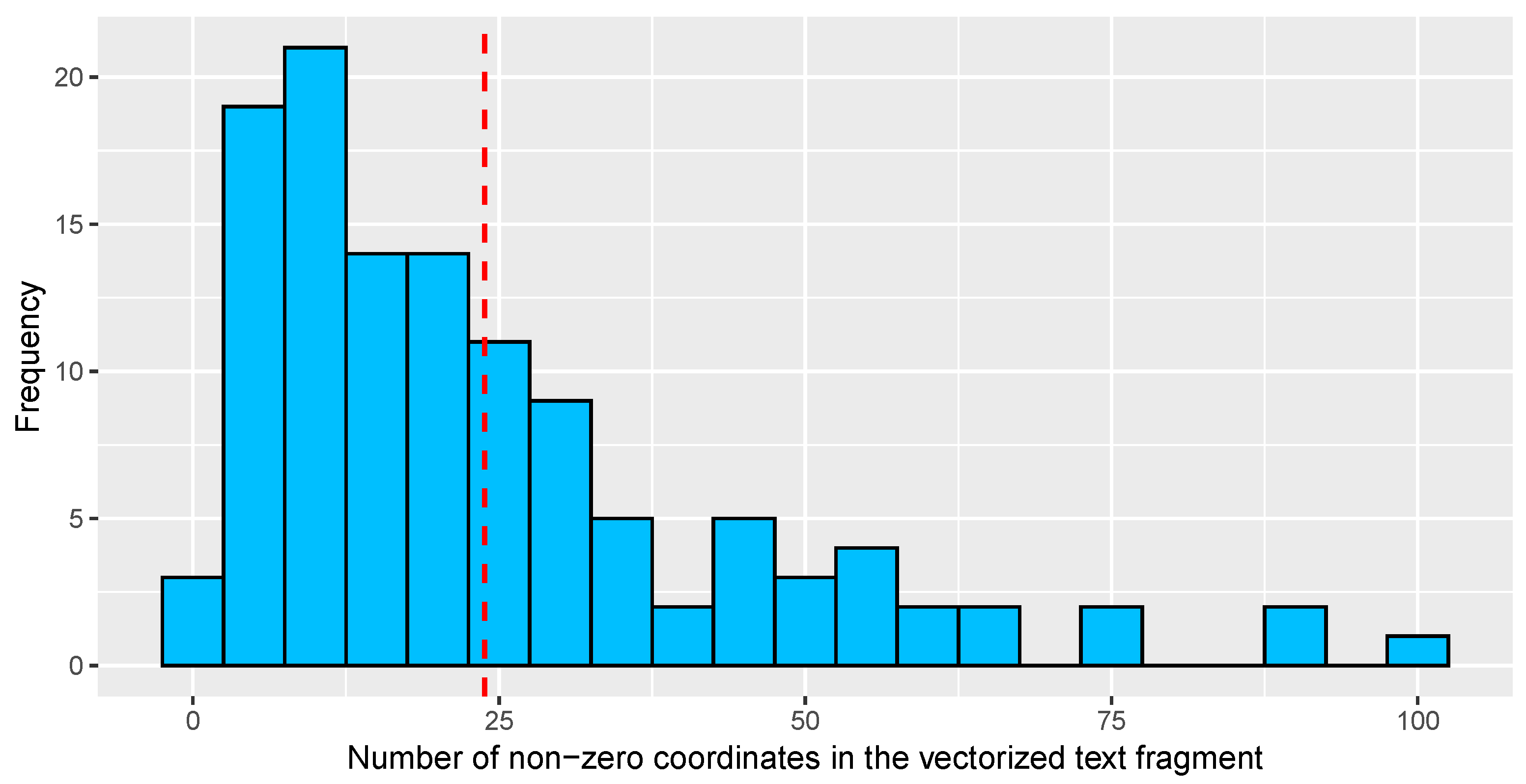
• It allows transforming variable length text fragments into fixed length numerical vectors through a vectorization process based on the tf-idf statistic [52]. The length of these numerical vectors is exactly the number of unique words in the corpus or set of text fragments considered in each case (see [25] for further details). For instance, if the training set is composed of 848 unique words, as is the case in Section 4, each text fragment is transformed into a vector in ${\mathbb{R}}^{848}$ whose coordinates are the values of the tf-idf statistic of each unique word (which depends both on the text fragment and the corpus under consideration) sorted alphabetically.

Therefore, once the set of text fragments that will constitute the training set is fixed, prior pre-processing allows the transformation into an $s\times (h+1)$ matrix whose rows are the h-dimensional vectors (where h is the number of unique words in the training set) representing the various text fragments $D_1,\dots ,D_s$ in the training set, along with the corresponding label. In short, the above pre-processing enables the transformation of text datasets into multivariate data.

One of the objectives of the analysis conducted in [25] was to study to what extent it is necessary to manually code the text fragments constituting the participant transcription, so that the labels of the remaining text fragments can be successfully predicted using well-known supervised classification methods. In doing so, the qualitative researcher would be offered a validated approach to speed up the coding process because the proposed method outputs a class label for each text fragment that indicates if the considered text fragment potentially contains a CFIR construct or not.

In [25], different case studies are analyzed depending on the amount of text fragments used in the training set. In that paper, we conclude that manually coding just the first 65% of the participants’ transcription is enough to automatically label the remaining 35% with a success rate of more than 80% using ANNs, SVMs and LASSO. Henceforth, in order to compare the performance of the depth-based approaches with the results obtained using traditional machine learning methods, the training set here consists of the first 65% of the 184 text fragments that compose the entire dataset, while the test set comprises the remaining fragments. Thus, the training set is

$$\mathcal{T}:=\{D_1,\dots ,D_{119}\},$$

and the test sample is its complement

$$\mathcal{E}:=\{D_{120},\dots ,D_{184}\}.$$

Before proceeding, it is important to know that the number of unique words in the training set is 848. Therefore, using the pre-processing described above and in ([25], Section 3), the training set is converted into a $119\times 849$ matrix and the test set is converted into a $65\times 849$ matrix.

3.2. Data Depths for Text Data

In the case study used in this manuscript, it would be very interesting to make use of a depth designed exclusively for dealing with text data. The reason is that, despite the fact that text datasets eventually become multivariate data, they are very specific multivariate data. Because the multivariate data are obtained from text vectorization via the tf-idf statistic, they are, for instance, very sparse. Figure 2 shows the sparsity of the vectorized training sample. In particular, it follows that, on average, each vector representing a text fragment in the training set has approximately 824 coordinates that are zero. This represents more than 97% of its entries.

To further describe the feature distribution of the dataset, Figure 3 displays a histogram containing the number of non-zero coordinates in the vectorized text fragments contained in the training sample. The plot illustrates the low amount of non-zero coordinates. The average of non-zero coordinates in the training sample is represented by the red dashed line with a value below 25.

Figure 4, in turn, shows a vectorized representation of two specific text fragments, $D_1$ and $D_7$, of the training set. Note that parallel coordinates [53] are used for the graphical representation. This figure helps to illustrate once again the sparsity of the dataset under study. Moreover, the latter representation suggests that the information of interest is actually concentrated in the peaks. Consequently, as can be seen in Section 4, conventional statistical depths designed for multivariate data do not produce competitive results with this type of data or, at the very least, the results are not optimized.

In an attempt to develop a statistical depth function for text data, the first possibility one may think of is to consider directional data on the sphere. The reason is that, in this type of data, it is not the magnitude of the different variables resulting from the tf-idf vectorization that is important, but the orientation of the vectorized text fragments in the feature space. Thus, the most similar observations would be expected to lie in the same region of the unit sphere, i.e., the angle between the vectors representing the two observations to be as parallel as possible. In order to achieve this, it would be enough to normalize each observation of the available data. In doing so, the observations would be transformed into points on the surface of the unit hypersphere, ${\mathbb{S}}^{p-1}$, where p is the dimension of the data under study.

This idea had already been explored in the literature. In [54], an analysis of distance-based depths for directional data was performed. There, the directional d-depth, which is a generalization of the above expressed idea, is introduced.

Definition 2

([54]). Let $\mathcal{F}$ be a distribution on ${\mathbb{S}}^{p-1}$. Let $d(·,·)$ be a bounded distance on ${\mathbb{S}}^{p-1}$ and let $d^{sup}:=sup\{d(\theta ,\varphi ):\theta ,\varphi \in {\mathbb{S}}^{p-1}\}$ be the upper bound of the distance between any two points on ${\mathbb{S}}^{p-1}$. Then, the directional d-depth of $\theta \in {\mathbb{S}}^{p-1}$ with respect to $\mathcal{F}$ is

$$D_d(\theta ,\mathcal{F}):=d^{sup}-E_{\mathcal{F}}\left[d(\theta ,Z)\right],$$

(3)

where $E_{\mathcal{F}}$ is the expectation under the assumption that Z has distribution $\mathcal{F}$.

Even though any bounded distance can be used in the previous definition, in [54] a proposal is made to consider rotation-invariant distances, i.e., distances satisfying $d(O\theta ,O\varphi )=d(\theta ,\varphi )$ for any $\theta ,\varphi \in {\mathbb{S}}^{p-1}$ and any $p\times p$ orthogonal matrix O. In particular, they suggest considering the chord distance depth, $D_{d_{\mathrm{chord}}}(·,·)$, which is the $d_{\mathrm{chord}}$-depth with $d_{\mathrm{chord}}(\theta ,\varphi ):={\parallel \theta -\varphi \parallel }_2=\sqrt{2(1-{\theta }^T\varphi )},$ for any $\theta ,\varphi \in {\mathbb{S}}^{p-1}.$

This proposal seems promising because, in principle, it would be expected to fit text data very well. Indeed, (3) has already been used to study patterns in text mining [55]. Moreover, it has been proved that chord distance depth has very good properties, e.g., that it is invariant to rotations (see Theorem 1 of [54]), or that there is a (non-unique) point which is the deepest (see Theorem 2 of [54]). However, as can be seen in Section 4, the results are not competitive in the dataset under study. Moreover, because the data are very sparse, the same is likely to occur when applying any existing statistical depth function without a prior transformation of the data.

3.2.1. Compositional Depth: The Inverse Fourier Transform

We propose a radically different alternative to deal with text data. It is inspired by signal theory and consists of using the inverse Fourier transform of the vectorized text fragments and then applying a statistical depth function for functional data. To the best of our knowledge, this methodology has not been considered in the literature before.

It is well known that the Fourier transform is a useful tool to move from the time domain to the frequency domain. Similarly, the inverse Fourier transform allows the reverse transformation, i.e., from the frequency domain to the time domain. In a sense, the process of vectorizing a text fragment using the tf-idf statistic provides a representation in the frequency domain. Indeed, each entry of a vectorized text fragment represents the tf-idf statistic of one of the unique words in the corpus computed within the text fragment and the corpus under consideration, as discussed in Section 3 and further detailed in ([25], Section 3). Since the tf-idf statistic is precisely an approximate measure of the frequency of a word, it can be assumed that the vectorized representation of a text fragment is a frequency spectrum. Thus, by computing the modulus of the inverse Fourier transform, we obtain the representation of the text fragment in the “time domain”. In analogy to signal theory, this is equivalent to the transition from the frequency decomposition to the original signal. Thus, with this procedure, sparse multivariate data can be easily converted into non-sparse functional data, allowing the application of statistical depth functions for functional data. In the following, this composition is referred to as compositional depth.

Figure 5 shows the curves resulting from considering the modulus of the inverse Fourier transform applied to the vectorized text fragments shown in Figure 4. Furthermore, Figure 6 summarizes the proposal on which compositional depth is based. It is shown how, when considering the inverse Fourier transform, one goes from a very sparse comb-like representation to a representation that is no longer sparse.

This section concludes with the formal definition of the compositional depth, which makes use of the discrete inverse Fourier transform. The discrete inverse Fourier transform of $x:={(x_1,\dots ,x_p)}^{{}^{\prime }}\in {\mathbb{R}}^p\subset {\mathbb{C}}^p$ is given by

$$\begin{array}{cc}\hfill {\mathcal{F}}^{-1}:{\mathbb{R}}^p\subset {\mathbb{C}}^p& ⟶{\mathbb{C}}^p\hfill \\ \hfill x& ⟼\widehat{x}:={({\widehat{x}}_1,\dots ,{\widehat{x}}_p)}^{{}^{\prime }},\mathrm{with} {\widehat{x}}_j:={\displaystyle \frac{1}{p}}\sum _{k=1}^p{x}_k{e}^{i\frac{2\pi }{p}(k-1)j} \mathrm{for} j=1,\dots p.\hfill \end{array}$$

(4)

Definition 3

Let $x\in {\mathbb{R}}^p$ and let D be a statistical depth function. The compositional D-depth of x with respect to $P_X\in {\mathcal{BP}}_p$ is

$${\widehat{C}}_D(x,P):=D\left(\right|{\mathcal{F}}^{-1}\left(x\right){|}_e,P_{|{\mathcal{F}}^{-1}{\left(X\right)|}_e}):{\mathbb{R}}^p\times {\mathcal{BP}}_p⟼\mathbb{R},$$

(5)

where ${\mathcal{F}}^{-1}\left(x\right)$ is the discrete inverse Fourier transform of $x\in {\mathbb{R}}^p$ and ${|·|}_e:{\mathbb{C}}^p⟼{\mathbb{R}}^p$ is an operator that, given a complex vector, computes the module of each of its components.

Making use of the notation in (4), we have that ${\mathcal{F}}^{-1}\left(x\right)=Wx,$ where $W:={\left(W_{jk}\right)}_{j,k=1,\dots p}$ is a matrix with entries in the complex numbers

$$W_{jk}={\displaystyle \frac{1}{p}}{e}^{i\frac{2\pi }{p}(k-1)j}.$$

If W were to have real entries and D in Definition 3 would be a multivariate depth satisfying the corresponding properties (Definition 1), applying W would not affect the results. That is because of the affine invariance property, which implies that $D(Wx,P_{WX})=D(x,P_X)$ for any non-singular matrix W in the real numbers.

A notion of depth, with the corresponding properties, for the complex numbers do not yet exist in the literature. Therefore, Definition 3 proposes to make use of the module operator, which results in

$$|{\mathcal{F}}^{-1}\left(x_j\right){|}_e={\displaystyle \frac{1}{p}}{\{\parallel x\parallel }^2+2\sum _{k,l=1;k\ne l}^p{x}_k{x}_{l}cos\left[i\frac{2\pi }{p}j(k-l)\right]{\}}^{1/2}forj=1,\dots p,$$

where $\parallel ·\parallel$ denotes the Euclidean norm. Having applied this module greatly increases the difficulty in studying the satisfaction of the depth properties. Note, however, that it is customary in the statistical depth area to call a function a depth function if it orders data, regardless of whether or not it satisfies all of the properties of the notion in the corresponding space. This is due to the fact that, for multivariate and functional spaces, depth instances were published before the corresponding notion of depth was provided.

Considering that $|{\mathcal{F}}^{-1}{\left(x\right)|}_e\in {\mathbb{R}}^p$ for each $x\in {\mathbb{R}}^p,$ it could be logical to select for $D(·,·)$ in (5) a multivariate depth (Definition 1). However, taking into account that, in practice, the elements in a functional space are not fully observed, being observed only at a finite set of discretization points, both the frequency and the time domain in (5) could be considered as functions, with ${\mathcal{F}}^{-1}(·)$ the inverse Fourier transform. We follow this reasoning in Section 4 when making use of functional depths.

4. Results

This section is devoted to reporting the results obtained by applying the depth-based classification methods to the dataset under study. Furthermore, a comparative study between these results and those obtained in [25] using more traditional supervised classification techniques is conducted. At this point, the reader is reminded that:

• The training set, $\mathcal{T}$, consists of the first 65% of the text fragments in the entire dataset and the test set, $\mathcal{E}$, is its complement. In particular, the training set consists of 119 observations. It is worth noting that the distribution of observations in this training dataset is relatively balanced, with 66 observations labeled as “1” (indicating the presence of at least one associated CFIR construct) and 53 labeled as “0” (indicating the absence of an associated CFIR construct). This results in a proportion of 55.5% of the training sample being labeled as “1” and 44.5% being labeled as “0”. The balanced nature of the data suggests that the model’s performance may not be significantly impacted by imbalanced class distribution, which can often be a concern when working with classification tasks. For further details, see Section 3.1.
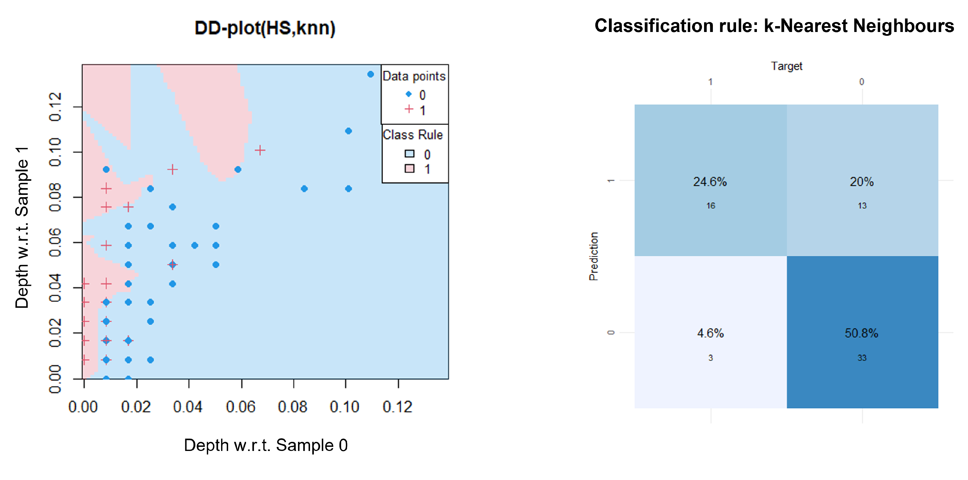
• A text fragment belongs to class 1 if it has at least one CFIR construct assigned to it. Conversely, an observation belongs to class 0 if a CFIR construct is not allocated to it.

First, the $D{D}^G$-classifier is applied directly to the multivariate data resulting from the vectorization of the original dataset (no Fourier transform is performed yet). In particular, two depth functions for multivariate data (the HS depth and the Mahalanobis depth [56]) and different classification rules (kNN, linear discriminant analysis and the maximum depth classifier) are used. Among the used combinations, it was found that the $D{D}^G$-classifier with the HS depth and the kNN (the choice of k is made by cross-validation) as the classification rule gives the least misclassification rate in the training sample, which is 0.17, and in the test sample, 0.25. These results are included in

Table 1. Summary table including the results obtained in the analysis carried out in this manuscript, and those obtained in [25] using LASSO, SVMs, ANNs and DT for 65/35% training–test split. The first column indicates the used classifier, the second column indicates the misclassification rate in the training sample and the third column indicates the misclassification rate in the test sample. The row in bold refers to the classifier that performed best in the test sample.

Classifier	Misclassification Rate (Training Sample)	Misclassification Rate (Test Sample)
LASSO	–	0.11
SVMs	–	0.14
ANNs	–	0.17
DTs	–	0.22
DD${}^G$-classifier(HS, maxD)	0.27	0.68
DD${}^G$-classifier(HS, lda)	0.29	0.31
DD${}^G$-classifier(HS, knn)	0.17	0.25
DD${}^G$-classifier(MhD, maxD)	0.29	0.49
DD${}^G$-classifier(MhD, lda)	0.23	0.71
DD${}^G$-classifier(MhD, knn)	0.25	0.69
DD${}^G$-classifier(ChordDist, RF)	0.16	0.38
DD${}^G$-classifier(ChordDist, knn)	0.21	0.46
DD${}^G$-classifier(compFM, maxD)	0.35	0.17
DD${}^G$-classifier(compFM, lda)	0.29	0.15
DD${}^G$-classifier(compFM, knn)	0.34	0.25
DD${}^G$-classifier(compRP, maxD)	0.35	0.18
DD${}^G$-classifier(compRP, lda)	0.32	0.09
DD${}^G$-classifier(compRP, knn)	0.38	0.31
DD${}^G$-classifier(compHS, maxD)	0.34	0.17
DD${}^G$-classifier(compHS, lda)	0.36	0.37
DD${}^G$-classifier(compHS, knn)	0.38	0.32

. In addition, Figure 7 displays the results of the combination of HS depth and kNN in more detail.

The blue points and red crosses in the DD-plot (left plot of Figure 7) represent the observations in the training sample and indicate the class to which they belong. In this case, the red crosses correspond to class 1, and the blue points to class 0. Similarly, the background image is light blue or light red, and represents the classification rule induced, in this case, by kNN. In particular, test data points would be assigned to class 1 if they fall into the light red regions when plotted, and to class 0 if they fall into the light blue ones. Note that, in this particular case, we observe less than 119 points/crosses in the DD-plot, which is precisely the training sample size. The reason is that some observations in the training sample have the same halfspace depth and, therefore, are superimposed (this is clearly illustrated when there is a cross over a point). However, even if it is not possible to distinguish them, they have been taken into account in the training process. Lastly, when we say Depth with respect to Sample 1 we mean that the depth is computed with regard to the distribution originated by the training observations belonging to class 1. The same applies to Depth with respect to Sample 0 and class 0.

The right plot of Figure 7 represents the confusion matrix that results from applying the latter procedure to the test sample. It follows from the confusion matrix in Figure 7 that the prediction accuracy of the $D{D}^G$-classifier(HS,kNN) applied directly to the vectorized test sample is 75%. Thus, all the traditional supervised classification methods analyzed in ([25], Section 5) outperform this depth-based proposal, as can be seen in the row labeled with a percentage 65% of Tables 5 and 6 of [25], where the accuracies in classifying the test sample for the methods LASSO, SVM, ANN and DT are 89%, 86%, 83% and 78%, respectively. In order to make this manuscript self-contained, Table 1 also includes the results obtained in [25] with LASSO, SVMs, ANNs and DTs for the same 65/35% training–test split. In particular, for each classification method, we report the misclassification rates in both training and test samples.

Next, the $D{D}^G$-classifier using the chord distance depth is analyzed. The results are shown in Figure 8. There, the DD-plot using the chord distance depth (left plot), and the confusion matrix that results from applying random forests (RF) classifier to the test sample (right plot) are represented. The red and blue points indicate whether the training observations belong to class 1 or 0, respectively. Moreover, the green crosses are the test observations belonging to class 1, while the orange ones are the test observations belonging to class 0.

As observed in the DD-plot in Figure 8, the maximum depth classifier (the main diagonal) achieves complete separation between groups for the training sample. However, it is clear that the performance drops dramatically for the test sample, since the maximum depth classifier assigns most test observations to class 1. Consequently, other classification rules were tested, namely: kNN and random forests. Among these, random forests provided the best performance for the training sample, achieving an out-of-bag error (the error of the data not selected in the bootstrap sampling process and therefore not used to grow the trees, see ([49], Chapter 15) for further details on random forests) of 0.84%. However, this particular case shows a clear example of overfitting, as the training sample is classified almost perfectly, but the misclassification rate for the test sample drastically increases to 0.38 (as can be inferred from the confusion matrix in Figure 8; and reported in Table 1). Thus, the conventional supervised classification methods analyzed in ([25], Section 5) outperform the $D{D}^G$-classifier(ChordDist,RF).

Finally, the $D{D}^G$-classifier is applied in combination with the compositional D-depth, that is, being D a statistical depth function applied to the functional data resulting from considering the modulus of the inverse Fourier transform of the vectorized dataset. Specifically, the compositional D-depth is used together with FM depth, RP depth and HS depth. The best results were obtained with FM depth and RP depth. They are shown in Figure 9. Note that the selected classification rules are the ones that have the lowest misclassification rates among the analyzed rules (maximum depth classifier, linear discriminant analysis and kNN) within the training sample. In particular, the $D{D}^G$-classifier(compFM,lda) has a misclassification rate of 0.29 in the training sample, and that of the $D{D}^G$-classifier(compRP,lda) is 0.32. These results are reported in Table 1.

Based on the confusion matrix in the top-right corner of Figure 9, it follows that the prediction accuracy of the $D{D}^G$-classifier(compFM,lda) in the test sample is 85%. This means that its performance is comparable to that of SVM (which was 86%), and is better than the scores obtained by the decision tree and ANN (which were 78% and 83%, respectively). Similarly, the confusion matrix in the bottom-right corner of Figure 9 shows that the prediction accuracy of the $D{D}^G$-classifier(compRP,lda) in the test sample is 91%. Therefore, this setting is more generalizable and outperforms the results obtained with all classifiers analyzed in [25] for this particular training–test split of text fragments, where the best prediction accuracy in the test sample was achieved by LASSO and was 89%.

In addition to the misclassification rate, the following performance metrics are also reported in order to assess the overall effectiveness: precision, recall, F1-score, and the area under the ROC curve (AUC). These results are displayed in

Table 2. Table summarizing the performance of the $D{D}^G$-classifier using compositional FM-depth (Columns 2 and 3) and compositional RP-depth (Columns 4 and 5), with linear discriminant analysis as the classification rule. Column 1 lists the type of metric, while Columns 2 and 4 show the results of the metrics for the training sample and Columns 3 and 5 show the results for the test sample.

	DD${}^{\mathit{G}}$-Classifier (compFM, lda)		DD${}^{\mathit{G}}$-Classifier (compRP, lda)
Metric	Training Sample	Test Sample	Training Sample	Test Sample
Misclassification rate	0.29	0.15	0.32	0.09
Precision	0.71	0.71	0.71	0.88
Recall	0.80	0.79	0.76	0.79
F1-score	0.75	0.75	0.74	0.83
AUC	0.69	0.83	0.69	0.85

, where Column 1 lists the type of performance metric. The results for the $D{D}^G$-classifier with linear discriminant analysis using compositional FM-depth in the training and test samples are shown in Columns 2 and 3, respectively. Similarly, the results for the $D{D}^G$-classifier using compositional RP-depth in the training and test samples are shown in Columns 4 and 5, respectively.

Overall, the $D{D}^G$-classifier using compositional FM-depth and/or RP-depth has demonstrated good performance based on the evaluation metrics of precision, recall, F1 score, and misclassification rate. Precision measures the proportion of correctly classified positive samples out of all samples classified as positive, with a value of around 0.7 indicating that the classifier is correctly identifying approximately 70% of the positive samples. Recall measures the proportion of correctly classified positive samples out of all actual positive samples, with a value of around 0.8, suggesting that the classifier is correctly identifying approximately 80% of the actual positive samples. The F1-score is a combination of precision and recall, and a value of around 0.75 indicates a good balance between the two. The AUC is a metric that measures the model’s ability to distinguish between positive and negative samples, with a higher value indicating better performance. In this case, the AUC is around 0.69 in the training sample and 0.8 in the test sample, indicating good performance in both cases. The slightly higher values for the performance metrics in the test sample suggest that the model may have slightly better generalizability, or ability to perform well on unseen data.

Consequently, the use of depth-based classifiers such as the $D{D}^G$-classifier together with the newly proposed compositional D-depth provides better results than conventional supervised classification techniques such as LASSO, SVMs, ANNs or DTs. Likewise, the classifiers based on the compositional D-depth rather than on ordinary statistical depths are more generalizable, as the misclassification rates in the test sample are lower. These results are promising for the use of this approach based in the compositional depth in text classification problems, not necessarily limited to healthcare-related data.

5. Conclusions

This manuscript introduces the compositional D-depth, a new concept of statistical depth function appropriate for text data. This statistical depth arises from the need to find a specific depth for handling text datasets, especially when text fragments are vectorized with the tf-idf statistic. The reason is that the previous vectorization process has been shown to result in very sparse datasets, hindering the application of other known statistical data depths.

The proposed depth is inspired by signal theory and consists of the composition of a known statistical depth function and the inverse discrete Fourier transform. This particular process allows very sparse datasets to be transformed into curves so that statistical depths for functional data can be applied to them. The rationale is that the inverse Fourier transform is a tool to move from frequency space (in a sense, the space defined by the tf-idf statistic) to time space.

In order to show the potential value of the compositional D-depth, a proof-of-concept analysis is conducted using qualitative data from the healthcare sector that has already been analyzed in [25] using traditional supervised classification methods such as ANNs, LASSO, SVMs and DTs. The case study analyzed in this manuscript—and also in [25]—revolves around a binary classification problem, which involves predicting whether or not a text fragment is assigned a CFIR construct. Explaining the process of converting qualitative data into quantitative data so that it can be used as input to classification methods is beyond the scope of this paper, but is described in detail in ([25], Section 3). It is worth mentioning, however, that given a training set consisting of s text fragments and containing h unique words, the output of the above pre-processing is an $s\times (h+1)$ matrix, whose rows are the vectorized representation of each text fragment (using the tf-idf statistic) along with its corresponding label (1 if it has been assigned at least one CFIR construct, or 0 if not). In the present case, the training sample consisted of the first 65% of the text fragments in the participants’ transcription, while the test sample consisted of the remaining 35%.

In this manuscript, the approach to the above binary classification problem is based on the application of the $D{D}^G$-classifier (see Section 2). Even though this depth-based classification method has been applied with different well-known statistical depths, the best results have been obtained by combining the $D{D}^G$-classifier with the newly defined compositional D-depth. In particular, the most favorable situation is obtained when considering the compositional depth together with the random projection depth $\left({\widehat{C}}_{RP}\right)$, as well as linear discriminant analysis as the classification rule for the DD-plots. The previous setup yields a success rate of 91% for the 65/35% training–test split under study. The results so far show not only that compositional depth works well on the text dataset under study, but also that it outperforms the results obtained using all other tested traditional machine learning methods (see [25], Section 5) for more details). In addition, it was found to be a great improvement over other statistical data depths, such as those developed for multivariate data or based on directional data on the hypersphere.

The results obtained in this proof-of-concept analysis are promising and highlight the utility of the compositional D-depth for dealing with text datasets. Furthermore, the analysis conducted in this manuscript leaves the door open to apply the same depth-based methodology to other text datasets that are not necessarily from the healthcare sector and, in general, to any dataset that is very sparse.

Future work will also include the study of the theoretical properties of the newly defined compositional D-depth. The study of these properties will lead to determine other applications in which the compositional D-depth could be successfully used.

References

1. Kowsari, K.; Jafari Meimandi, K.; Heidarysafa, M.; Mendu, S.; Barnes, L.; Brown, D. Text Classification Algorithms: A Survey. Information 2019, 10, 150. [Google Scholar] [CrossRef] [Green Version]
2. Indurkhya, N. Emerging Directions in Predictive Text Mining. WIREs Data Min. Knowl. Discov. 2015, 5, 155–164. [Google Scholar] [CrossRef]
3. Chowdhary, K.R. Natural Language Processing. In Fundamentals of Artificial Intelligence; Chowdhary, K.R., Ed.; Springer: New Delhi, India, 2020; pp. 603–649. ISBN 978-81-322-3972-7. [Google Scholar]
4. Vijayakumar, B.; Fuad, M.M.M. A New Method to Identify Short-Text Authors Using Combinations of Machine Learning and Natural Language Processing Techniques. Procedia Comput. Sci. 2019, 159, 428–436. [Google Scholar] [CrossRef]
5. Osorio, J.; Beltran, A. Enhancing the Detection of Criminal Organizations in Mexico Using ML and NLP. In Proceedings of the 2020 International Joint Conference on Neural Networks (IJCNN), Glasgow, UK, 19–24 July 2020; pp. 1–7. [Google Scholar]
6. Gupta, S.; Nishu, K. Mapping Local News Coverage: Precise Location Extraction in Textual News Content Using Fine-Tuned BERT Based Language Model. In Proceedings of the Fourth Workshop on Natural Language Processing and Computational Social Science, Online, 20 November 2020; pp. 155–162. [Google Scholar]
7. Kastrati, Z.; Dalipi, F.; Imran, A.S.; Pireva Nuci, K.; Wani, M.A. Sentiment Analysis of Students’ Feedback with NLP and Deep Learning: A Systematic Mapping Study. Appl. Sci. 2021, 11, 3986. [Google Scholar] [CrossRef]
8. Hossain, A.; Karimuzzaman, M.; Hossain, M.M.; Rahman, A. Text Mining and Sentiment Analysis of Newspaper Headlines. Information 2021, 12, 414. [Google Scholar] [CrossRef]
9. Rajput, A. Chapter 3 - Natural Language Processing, Sentiment Analysis, and Clinical Analytics. In Innovation in Health Informatics; Lytras, M.D., Sarirete, A., Eds.; Next Gen Tech Driven Personalized Med&Smart Healthcare; Academic Press: Cambridge, MA, USA, 2020; pp. 79–97. ISBN 978-0-12-819043-2. [Google Scholar]
10. Alnazzawi, N.; Alsaedi, N.; Alharbi, F.; Alaswad, N. Using Social Media to Detect Fake News Information Related to Product Marketing: The FakeAds Corpus. Data 2022, 7, 44. [Google Scholar] [CrossRef]
11. Hvitfeldt, E.; Silge, J. Supervised Machine Learning for Text Analysis in R, 1st ed.; CRC Press: New York, NY, USA, 2021. [Google Scholar]
12. Haynes, C.; Palomino, M.A.; Stuart, L.; Viira, D.; Hannon, F.; Crossingham, G.; Tantam, K. Automatic Classification of National Health Service Feedback. Mathematics 2022, 10, 983. [Google Scholar] [CrossRef]
13. Fan, H.; Du, W.; Dahou, A.; Ewees, A.A.; Yousri, D.; Elaziz, M.A.; Elsheikh, A.H.; Abualigah, L.; Al-qaness, M.A.A. Social Media Toxicity Classification Using Deep Learning: Real-World Application UK Brexit. Electronics 2021, 10, 1332. [Google Scholar] [CrossRef]
14. Rish, I. An Empirical Study of the Naïve Bayes Classifier. In Proceedings of the International Joint Conference on Artificial Intelligence: Workshop on Empirical Methods in Artificial Intelligence, Seattle, WA, USA, 4–10 August 2001; pp. 41–46. [Google Scholar]
15. Kuhn, M.; Johnson, K. Applied Predictive Modeling, 1st ed.; Springer: New York, NY, USA, 2013. [Google Scholar]
16. Hastie, T.; Tibshirani, R. Statistical Learning with Sparsity, 1st ed.; CRC Press: New York, NY, USA, 2015. [Google Scholar]
17. Boser, B.; Guyon, I.; Vapnik, V. A training algorithm for optimal margin classifiers. In Proceedings of the Fifth Annual Workshop on Computational Learning Theory, Pittsburgh, PA, USA, 27–29 July 1992. [Google Scholar]
18. Cristianini, N.; Shawe-Taylor, J. An Introduction to Support Vector Machines and Other Kernel-Based Learning Methods; Cambridge University Press: Cambridge, UK, 2000; Available online: www.support-vector.net (accessed on 20 May 2022).
19. Kim, S.M.; Han, H.; Park, J.M.; Choi, Y.J.; Yoon, H.S.; Sohn, J.H.; Baek, M.H.; Kim, Y.N.; Chae, Y.M.; June, J.J.; et al. A Comparison of Logistic Regression Analysis and an Artificial Neural Network Using the BI-RADS Lexicon for Ultrasonography in Conjunction with Introbserver Variability. J. Digit. Imaging 2012, 25, 599–606. [Google Scholar] [CrossRef]
20. Elman, J.L. Finding structure in time. Cogn. Sci. 1990, 14, 179–211. [Google Scholar] [CrossRef]
21. Collobert, R.; Weston, J.; Bottou, L.; Karlen, M.; Kavukcuoglu, K.; Kuksa, P. Natural language processing (almost) from scratch. J. Mach. Learn. Res. 2011, 12, 2493–2537. [Google Scholar]
22. Kalchbrenner, N.; Blunsom, P. Recurrent convolutional neural networks for discourse compositionality. In Proceedings of the Workshop on Continuous Vector Space Models and their Compositionality, Sofia, Bulgaria, 9 August 2013; pp. 119–126. [Google Scholar]
23. Aldjanabi, W.; Dahou, A.; Al-qaness, M.A.A.; Elaziz, M.A.; Helmi, A.M.; Damaševičius, R. Arabic Offensive and Hate Speech Detection Using a Cross-Corpora Multi-Task Learning Model. Informatics 2021, 8, 69. [Google Scholar] [CrossRef]
24. Lee, E.; Lee, C.; Ahn, S. Comparative Study of Multiclass Text Classification in Research Proposals Using Pretrained Language Models. Appl. Sci. 2022, 12, 4522. [Google Scholar] [CrossRef]
25. Bolívar, S.; Nieto-Reyes, A.; Rogers, H.L. Supervised Classification of Healthcare Text Data Based on Context-Defined Categories. Mathematics 2022, 10, 2005. [Google Scholar] [CrossRef]
26. Najafabadi, M.M.; Villanustre, F.; Khoshgoftaar, T.M.; Seliya, N.; Wald, R.; Muharemagic, E. Deep Learning Applications and Challenges in Big Data Analytics. J. Big Data 2015, 2, 1. [Google Scholar] [CrossRef] [Green Version]
27. Akhtar, M.S.; Sawant, P.; Sen, S.; Ekbal, A.; Bhattacharyya, P. Solving Data Sparsity for Aspect Based Sentiment Analysis Using Cross-Linguality and Multi-Linguality. In Proceedings of the 2018 Conference of the North American Chapter of the Association for Computational Linguistics: Human Language Technologies, Volume 1 (Long Papers), New Orleans, LA, USA, 1–6 June 2018; pp. 572–582. [Google Scholar]
28. Pervaiz, A.; Hussain, F.; Israr, H.; Tahir, M.A.; Raja, F.R.; Baloch, N.K.; Ishmanov, F.; Zikria, Y.B. Incorporating Noise Robustness in Speech Command Recognition by Noise Augmentation of Training Data. Sensors 2020, 20, 2326. [Google Scholar] [CrossRef] [Green Version]
29. Zhang, Y.; Jin, R.; Zhou, Z.-H. Understanding Bag-of-Words Model: A Statistical Framework. Int. J. Mach. Learn. Cyber. 2010, 1, 43–52. [Google Scholar] [CrossRef]
30. Landauer, T.K.; Foltz, P.W.; Laham, D. An Introduction to Latent Semantic Analysis. Discourse Process. 1998, 25, 259–284. [Google Scholar] [CrossRef]
31. Chatterjee, N.; Sahoo, P.K. Random Indexing and Modified Random Indexing Based Approach for Extractive Text Summarization. Comput. Speech Lang. 2015, 29, 32–44. [Google Scholar] [CrossRef]
32. Weinberger, K.; Dasgupta, A.; Attenberg, J.; Langford, J.; Smola, A. Feature Hashing for Large Scale Multitask Learning. In Proceedings of the 26th Annual International Conference on Machine Learning, Montreal, QC, Canada, 14–18 June 2009. [Google Scholar]
33. Drikvandi, R.; Lawal, O. Sparse Principal Component Analysis for Natural Language Processing. Ann. Data Sci. 2020. [Google Scholar] [CrossRef]
34. Serfling, R.; Zuo, Y. General Notions of Statistical Depth Function. Ann. Stat. 2000, 28, 461–482. [Google Scholar] [CrossRef]
35. Nieto-Reyes, A.; Battey, H. A Topologically Valid Definition of Depth for Functional Data. Stat. Sci. 2016, 31, 61–79. [Google Scholar] [CrossRef]
36. González-De La Fuente, L.; Nieto-Reyes, A.; Terán, P. Statistical Depth for Fuzzy Sets. Fuzzy Sets Syst. 2022, 443, 58–86. [Google Scholar] [CrossRef]
37. Cuesta-Albertos, J.A.; Febrero-Bande, M.; Oviedo, M. The DDG-Classifier in the Functional Setting. Test 2017, 26, 119–142. [Google Scholar] [CrossRef] [Green Version]
38. Rogers, H.L.; Pablo-Hernando, S.; Núñez-Fernández, S. Barriers and facilitators in the implementation of an evidence-based health promotion intervention in a primary care setting: A qualitative study. J. Health Organ. Manag. 2021, 35, 349–367. [Google Scholar] [CrossRef]
39. Fraiman, R.; Muniz, G. Trimmed Means for Functional Data. Test 2001, 10, 419–440. [Google Scholar] [CrossRef]
40. Cuevas, A.; Febrero, M.; Fraiman, R. Robust Estimation and Classification for Functional Data via Projection-Based Depth Notions. Comput. Stat. 2007, 22, 481–496. [Google Scholar] [CrossRef]
41. Hlubinka, D.; Gijbels, I.; Omelka, M.; Nagy, S. Integrated Data Depth for Smooth Functions and Its Application in Supervised Classification. Comput. Stat. 2015, 30, 1011–1031. [Google Scholar] [CrossRef] [Green Version]
42. Tukey, J.W. Mathematics and picturing of data. Proc. ICM Vanc. 1975, 2, 523–531. [Google Scholar]
43. Cuesta-Albertos, J.A.; Nieto-Reyes, A. The Random Tukey Depth. Comput. Stat. Data Anal. 2008, 52, 4979–4988. [Google Scholar] [CrossRef]
44. Cuesta-Albertos, J.; Nieto-Reyes, A. Albertos, J.; Nieto-Reyes, A. A Random Functional Depth. In Functional and Operatorial Statistics; Dabo-Niang, S., Ferraty, F., Eds.; Physica-Verlag HD: Heidelberg, Germany, 2008; pp. 121–126. [Google Scholar]
45. Mosler, K.; Hoberg, R. Data analysis and classification with the zonoid depth. Amer. Math. Soc. DIMACS Ser. 2006, 72, 49–59. [Google Scholar]
46. Liu, R.Y. On a Notion of Data Depth Based on Random Simplices. Ann. Stat. 1990, 18, 405–414. [Google Scholar] [CrossRef]
47. Liu, R.Y.; Parelius, J.M.; Singh, K. Multivariate Analysis by Data Depth: Descriptive Statistics, Graphics and Inference, (with Discussion and a Rejoinder by Liu and Singh). Ann. Stat. 1999, 27, 783–858. [Google Scholar] [CrossRef]
48. Li, J.; Cuesta-Albertos, J.A.; Liu, R.Y. DD-Classifier: Nonparametric Classification Procedure Based on DD-Plot. J. Am. Stat. Assoc. 2012, 107, 737–753. [Google Scholar] [CrossRef]
49. Hastie, T.; Tibshirani, R.; Friedman, J.H. The Elements of Statistical Learning: Data Mining, Inference, and Prediction, 1st ed.; Springer: New York, NY, USA, 2001. [Google Scholar]
50. Cover, T.; Hart, P. Nearest Neighbor Pattern Classification. IEEE Trans. Inf. Theory 1967, 13, 21–27. [Google Scholar] [CrossRef] [Green Version]
51. Damschroder, L.J.; Aron, D.C. Fostering implementation of health services research findings into practice: A consolidated framework for advancing implementation science. Implement. Sci. 2009, 4, 50. [Google Scholar] [CrossRef] [Green Version]
52. Manning, C.D.; Raghavan, P. Introduction to Information Retrieval, 1st ed.; Cambridge University Press: New York, NY, USA, 2008. [Google Scholar]
53. Inselberg, A.; Dimsdale, B. Parallel Coordinates: A Tool for Visualizing Multi-Dimensional Geometry. In Proceedings of the Proceedings of the First IEEE Conference on Visualization: Visualization ‘90, San Francisco, CA, USA, 23–26 October 1990; pp. 361–378. [Google Scholar]
54. Pandolfo, G.; Paindaveine, D.; Porzio, G.C. Distance-Based Depths for Directional Data. Can. J. Stat. 2018, 46, 593–609. [Google Scholar] [CrossRef]
55. Hornik, K.; Feinerer, I.; Kober, M.; Buchta, C. Spherical K-Means Clustering. J. Stat. Softw. 2012, 50, 1–22. [Google Scholar] [CrossRef]
56. Mahalanobis, P.C. On the Generalized Distance in Statistics; National Institute of Science of India: Calcutta, India, 1936. [Google Scholar]
Figure 1. Block diagram representing the steps followed to obtain and validate the proposed depth function designed for text data.
Mathematics 11 00228 g001
Figure 2. Histogram showing the sparsity of the vectorized training set. The horizontal axis shows the number of coordinates that are zero in the vectors resulting from the vectorization of the text fragments conforming the training set, while the vertical axis shows the absolute frequency of occurrence. The red vertical dashed line represents the average number of coordinates that are zero in the vectorized text fragments that form the training set.
Mathematics 11 00228 g002
Figure 3. Histogram showing the small concentration of non-zero coordinates in the vectorized training set. The horizontal axis shows the number of coordinates that are non-zero in the vectors resulting from the vectorization of the text fragments conforming the training set, while the vertical axis shows the absolute frequency of occurrence. The red vertical dashed line represents the average number of coordinates that are non-zero in the vectorized text fragments that form the training set.
Mathematics 11 00228 g003
Figure 4. Vectorized representation of text fragments D 1 (red line) and D 7 (blue line) of the training set. Note that parallel coordinates are used. The horizontal axis represents each of the unique words in the training set sorted alphabetically (instead of the word itself, we represent the order number that results from sorting all words alphabetically, so that for example the word “a” is represented by a 1), while the vertical axis shows their tf-idf statistic.
Mathematics 11 00228 g004
Figure 5. Modulus of the inverse Fourier transform applied to the vectorized text fragments shown in Figure 4. Again, the red and blue curves correspond to the text fragments D 1 and D 7 of the training set.
Mathematics 11 00228 g005
Figure 6. Schematic representation of the idea behind the compositional depth. The upper part shows the frequency decomposition of a wave in the time domain via the Fourier transform (FT). The inverse is also represented (IFT). The lower part illustrates how the inverse Fourier transformation affect text fragments D 1 , in red, and D 7 , in blue, of the training set.
Mathematics 11 00228 g006
Figure 7. Results of applying the D D G -classifier(HS,kNN) to the multivariate text data (no Fourier transformation is performed yet). That is, the D D G -classifier with the HS depth and the kNN as the classification rule is used. The DD-plot (left plot) represents the training data and the confusion matrix (right plot) the test data.
Mathematics 11 00228 g007
Figure 8. Results of applying the D D G -classifier(ChordDist,RF) to the multivariate text data (no Fourier transform is performed yet). The DD-plot on the left uses the chord distance depth, and random forest as the classification rule. The right plot represents the confusion matrix resulting from applying the former procedure to the test sample. The red and blue points indicate whether the observations in the training sample belong to class 1 or 0, respectively. The green and orange crosses are the test observations corresponding to class 1 and 0, respectively.
Mathematics 11 00228 g008
Figure 9. Results of applying the D D G -classifier to the Fourier-transformed text data i.e., together with the compositional D-depth. The DD-plot in the upper left corner uses compositional FM-depth, while the DD-plot in the lower left corner uses compositional RP-depth. In both cases, linear discriminant analysis is used as the classification rule. The top right plot shows the confusion matrix that results when the D D G -classifier (compFM,lda) is applied to the test sample. Similarly, the bottom right plot shows the confusion matrix that results when the D D G -classifier (compRP,lda) is applied to the test sample.
Mathematics 11 00228 g009