Abstract
A new approach to the numerical study of arbitrary waveform impulses in a layered porous and fractured-porous medium in a two-dimensional formulation has been developed. Layers can have different characteristics and contain fractures. A computer implementation of the mathematical model based on the finite-difference MacCormack method has been completed. A number of test calculations have been carried out confirming the reliability of the numerical solutions obtained. The possibility of using the proposed approach to solve problems of wave dynamics is shown.
MSC:
76S05
1. Introduction
The problems of wave propagation in porous media and filtration are mainly solved numerically. At the same time, fluid filtration problems usually assume that the skeleton is stationary, and only fluid motion is considered. For example, in [1,2], a mathematical model is proposed that describes the process of pumping gas into a porous medium initially filled with methane and water. Methodology for solving the system of equations of the mathematical model has been constructed. The methodology has been tested; in the one-dimensional axisymmetric case, the calculation results have been compared with a self-similar solution for a perfect gas, showing a good qualitative and quantitative agreement. When solving wave problems, both a one-velocity model of a continuum is used (the velocities of the skeleton and the fluid coincide, the pressure in the media is the same) and a two-velocity model with two pressures (the velocities and pressures of the phases are different, and the force interphase interaction is taken into account). When studying wave processes in porous media with boundaries, a simpler one-velocity model of continuum is often used because of the complexity of the problem.
Let us briefly consider the methods for solving these problems. The Fourier method makes it possible to investigate the problem of the propagation and reflection of waves in a linear approximation in the framework of both a one-velocity and two-velocity model. The method can be successfully used for homogeneous media. For media with boundaries, its use is also possible [3], but in the case of several boundaries (two or more), the amount of calculations increases dramatically. For numerical modeling, various authors have used the methods of large particles, TVD, and Lax–Wendroff. In [4], the method of large particles was used to calculate the motion of a porous powdery medium. The TVD method was applied in [5] to calculate the motion of a two-phase mixture with different velocities and pressures of components, and the problem of the reflection of a shock wave from a wall in a mixture inhomogeneous in concentration was considered. The Lax–Wendroff method [6] in relation to the problem of the passage of the gas–porous medium interface by a wave and reflection from a rigid wall covered with a porous material is described in [7]. For the numerical study of the pressure wave propagation in a porous medium containing a two-layer waveguide, the Lax–Wendroff method was used in a two-dimensional axisymmetric formulation [8].
There are several works in the literature devoted to the study of wave propagation in fractured porous media. In [9], the theory of wave propagation in fractured porous media is presented. The equations of motion and constitutive equations were obtained by volume averaging the microscale balance and constitutive equations and by assuming small deformations. In the simplest case, the final set of equations were reduced to equations of the Biot’s theory. Propagation of monochromatic waves in a fractured porous medium saturated with two immiscible fluids was considered, but the behavior of the pulse perturbations was not studied.
In [10], a three velocity, three pressure mathematical model of a liquid-saturated deformable double porous medium was proposed, which allowed for studying the wave processes. The difference between the velocities and pressures of the liquid phase in the pore systems of different characteristic sizes, the exchange of liquid between the pore systems, and the non-stationary forces of the interphase interaction were taken into account. The mathematical model was a development of the model of a porous medium [11] and a fractured medium [12]. Dispersion dependences were constructed, phase velocities and linear damping decrements of three longitudinal and transverse waves were calculated, and parametric analysis was performed.
Up until now, the behavior of arbitrary waveform pulses in a layered porous and fractured porous medium in a two-dimensional formulation has not been studied.
In this paper, we propose the use of the finite-difference MacCormack calculation method [13] in relation to the problem of wave propagation in a layered porous medium, some layers of which may contain fractures. This problem was considered in a two-dimensional formulation. A computer implementation of the model was performed and preliminary calculations were carried out, which showed the effectiveness of the proposed methodology.
2. Mathematical Model
We use a three-velocity model of a fractured-porous medium [10], which, in the absence of fractures (q = 0, αfr = 0), describes the dynamics of a porous medium [11].
The equations of mass balance for each phase have the following form:
The momentum equations are
where are the reduced density, velocity, volume fraction of the j-th phase, respectively. The subscript s refers to the parameters of the skeleton; f to the fluid parameters of the primary pores; and fr to the fluid parameters in the larger, secondary pores or fractures. The superscripts i, k are coordinates indices; is the volume averaged (by pores and fractures) fluid pressure; are the reduced stresses in the skeleton, fluid pressure in the pores, and fractures, respectively; q is the intensity of the flow between the pore systems; is the permeability of the primary pore system; is the characteristic size of the pores or fractures; is the radius of the blocks; and is the dynamic viscosity of the fluid.
The interaction forces between the skeleton and the fluid in the pores and between the skeleton and the fluid in the fractures are taken as the sum of the forces of the associated masses and the viscous friction :
where is the true density of the j-phase, the subscript 0 denotes the unperturbed value of the parameter, and are the dimensionless coefficients of the phase interaction depending on the structure of the medium.
The skeleton of a porous medium is assumed to be elastic:
where are strains of the skeleton of the fractured porous medium, are elastic moduli.
For each of the phases, we take a linear constitutive equation in the acoustic approximation:
where is the true pressure in the solid phase, and are volume elastic moduli for the solid and fluid materials, respectively.
To close the system of equations, we use the relations between the true pressures in phases and the effective pressure in the skeleton , the relationship between the true and reduced densities, and the equation for varying the porosity inside the porous block:
The total stress in this medium is related to the averaged pressure in the fluid and the effective voltage in the skeleton by the formula
We believe that the porous medium consists of several layers, and some layers may also contain fractures. Layers can be saturated with various fluids, have different properties (densities and elastic moduli of phases, porosity, characteristic sizes of pores and fractures, and effective elastic moduli of the skeleton) and have different lengths.
The conditions at the boundaries of various porous media are usually described by one of three main types: open, partially open, or closed pores [14]. In relation to the wave propagation in the one-dimensional fluid-saturated porous phonon crystals, open and partial-open pore interfaces were considered in detail in [15,16].
In our work, at the boundaries of the layers, it was assumed that the condition of the “open pores” type was fulfilled, when there was free fluid exchange between the layers. At the same time, the problem of the propagation of pulse perturbations in a layered medium was considered in a two-dimensional formulation.
Thus, we consider the motion to be two-dimensional in the x, z plane, and the z axis is perpendicular to the boundaries of the layers. In this case, the boundary conditions for the open pores at the contacts of various porous media or a porous medium and fractured porous medium are reduced to the following conditions:
- Continuity of the skeleton velocity ,
- Continuity of fluid flow through the boundary (porous medium) and (fractured porous medium)
- Fluid pressure continuity (porous medium) and (fractured porous medium)
- Continuity of the components of the total stresses , which, in the case of open pores, means continuity of .
Thus, at the boundary between a porous medium (PM, ) and a fractured porous medium (FPM, ), the following continuity conditions are met:
If the porous medium (fractured porous medium) borders on the fluid, then the conditions of continuity of pressures and fluid flow through the boundary are valid. Also, the condition remains that the components of the effective stress in the skeleton (porous or fractured porous medium) are equal to zero. So, at the interface between the fluid () and porous medium (), the continuity conditions are
In addition, the case of two bordering fluids will be considered further as a test problem. In this simplest case, the conditions of continuity of velocities and pressures are met at the boundary of two fluids.
3. Numerical Integration Method
In the presented system of equations, we make the transition to dimensionless variables
where is the fluid density in the medium in which the perturbation is set.
Next, we omit the line over dimensionless variables.
Consider the two-dimensional (in x-z plane) motion of the fractured porous medium. The equations of the motion include partial differential equations and algebraic equations. The differential equations are represented as a single equation in matrix form:
For a finite-difference approximation of this equation, we apply the MacCormack method [13], with which the values of the variables will be calculated at the grid nodes, and the values of the remaining variables are then determined from the algebraic equations.
The numerical solution is constructed in the nodes of the computational grid
where τ, hx, and hz are the steps in time and space.
According to the MacCormack scheme [13], the numerical integration on each time layer consists of the following steps:
- The derivatives in space are approximated “downstream”, Q = 0
- The space derivatives are approximated “upstream”, Q = 0
- The resulting solution is in the form
- The resulting solution is corrected taking into account ≠ 0
Additional dummy cells are introduced at the boundaries of the calculation area (). The values of the unknowns in these cells are determined from the conditions
The time step should be much less than the characteristic time of the interphase interaction process and should satisfy the Courant–Friedrichs–Levy stability condition. The step in the space is selected according to the Runge method (recalculation with a half step).
The MacCormack method is a modification of the two-step Lax–Wendroff method [6], which is successfully used to solve wave problems in a porous medium. They are both explicit “predictor–corrector” methods of the second order of accuracy in time and space, and the through-count schemes. In the Lax–Wendroff scheme, at half-step in time , the values of the unknowns are calculated at the half-integer points .
Therefore, in the case of contact discontinuities, it is necessary to determine the effective values of the parameters (elastic moduli of phases and effective elastic moduli of skeleton) at such half-integer points. The advantage of the MacCormack method is that it does not require the calculation of these unknown effective parameters at half-integer points, so there is no such problem. This computational method refers to the through-count.
The fulfillment of continuity conditions at the boundaries of the layers is verified and confirmed by the output, and by verifying these quantities near the boundary nodes of the computational grid during the calculation process.
4. Results of Test Calculations
To validate the method, we chose two problems regarding the reflection/transmission of a pressure pulse at the boundary of two non-dissipative continuous media. These problems differ in the way the perturbation is initiated. In the first problem, the initial plane pulse of a triangular shape is given. Such a problem is essentially one-dimensional and has an analytical solution that determines the amplitudes of the reflected and transmitted waves. Comparison with such a solution allows one to check the numerical solution. In the second problem, the perturbation is given by a small size source. A short-term injection of fluid causes a pulse perturbation of pressure. In this case, the picture is essentially two-dimensional, its analysis allows us to check the efficiency of the method. Finally, the third task allows us to test the effectiveness of the method when calculating the reflection/transmission of a pressure pulse through the boundary between a porous medium and fractured-porous medium. In this case, the pressure perturbation is also created by the fluid source, as it is impossible to set the initial pressure pulse in a porous medium. To verify the calculation result, a comparison is performed with a one-dimensional case.
4.1. The Passage of a Traveling Plane Wave through the Boundary of Two Single-Phase Media
Here, we consider two bordering continuous media with different properties, liquid and gaseous. Area 1 (−1 m < z < 0, 0 < x < 0.2 m) is occupied by a single-phase medium with properties 1000 kg/m3, = 2.25 · 109 Pa, and sound velocity = 1500 m/s (water), and area 2 (0 < z < 0.5 m, 0 < x < 0.2 m) is a single-phase medium with properties 72 kg/m3, = 1.33 · 107 Pa, and = 430 m/s (methane, = 107 Pa). At the boundary between the media, the conditions of the continuity of velocities and pressures should be met. When calculating using this numerical method, these conditions are fulfilled automatically, which is proven and confirmed during the calculation process.
The initial perturbation is given in the area 1 in the form of a wave traveling in the positive direction of the z axis, while the overpressure is set , as well as the density and velocity of the medium particles associated with pressure by known ratios for traveling plane waves, namely,
In this case (Figure 1), a triangular pulse is
where = −0.81 m, = −0.57 m, = −0.51 m, and = 0.1 are given (Figure 1). So, pulse length is 0.3 m and its duration is 0.2 ms.
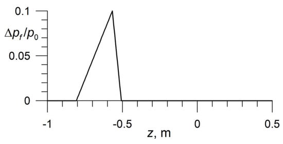
Figure 1.
The initial pressure perturbation.
In fact, such a perturbation causes one-dimensional motion of the medium along the z axis, which is confirmed by the results of the calculations (Figure 2). The pressure profiles in Figure 2a and the pressure fields in Figure 2b of a traveling plane wave for several time moments are shown. The color scale on the right (b) shows the pressure level . The pulse propagates through medium 1 without distortion (t = 0.1, 0.3 ms), then the reflected pulse in medium 1 and the transmitted pulse in medium 2 (t = 0.5, 0.8 ms) are observed. Figure 2c shows the time variation of the dimensionless overpressure at two points, before and after the boundary. The shape of both the reflected and the transmitted pulse repeats the original shape. The amplitudes of the initial, reflected, and transmitted waves shown in the Figure 2c correlate with the reflection and transmission coefficients calculated according to the theoretical formulas at the boundaries of two media, which values are −0.96 and 0.04, respectively.
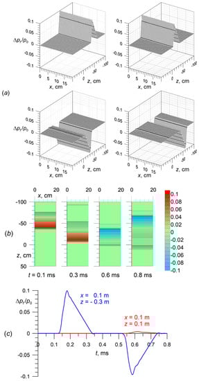
Figure 2.
The passage of a traveling plane wave through the boundary of two single-phase media. The profiles (a) and fields (b) of the dimensionless pressure difference when a traveling plane wave passes through the boundary of two single-phase media for several time points. The color scale on the right (b) shows the pressure level . Calculated “oscillograms” of pressure at two points for the first (blue line) and second (red line) media (c).
4.2. Propagation of the Perturbation from the Source and Its Passage/Reflection through the Boundary of Two Single-Phase Media
Let two model bordering continuous media with different properties be given again, but, unlike test 1, the perturbation is created by a source of liquid. Area 1 (−1.5 m < z < 0, 0 < x < 2 m) is occupied by a single-phase medium with properties of 1000 kg/m3, = 2.25 · 109 Pa, and = 1500 m/s, and area 2 (0 < z < 0.5 m, 0 < x < 2 m) is a single-phase medium with properties of 500 kg/m3, = 0.5⋅109 Pa, and = 1000 m/s.
At the initial moment, the media are at rest. A perturbation of a finite duration is given in area 1 by a source of the same fluid located in the square In this case, the source term should be added to the right side of the mass balance of Equation (1)
where is the volume of liquid that is injected into the source zone during time t, related to the volume of this zone.
In the calculations presented below, the dependence is taken as Figure 3
where = 2.475 · 10−3, = 20 ms−1, = 0.6, and = 2 kHz are given.
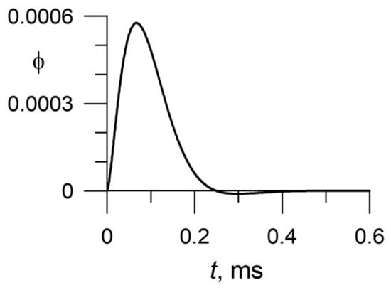
Figure 3.
The initial perturbation function .
In medium 1, at the initial stage, the perturbation from the source propagates radially symmetrically, with a constant velocity equal to the sound velocity in this medium. After the perturbation passes into area 2, the transmitted (in medium 2) and reflected (in medium 1) waves are observed (Figure 4). In medium 2, the velocity of the propagation of perturbation is also equal to the sound velocity in this medium. During propagation, the perturbation attenuates due to the geometry in proportion to the distance from the source. The pattern of propagation of the perturbation and reflection/transmission through the boundary indicates the correctness of the calculation results (Figure 4): the wave propagates radially, the amplitude decreases as it moves away from the source, the wave velocities are equal to the sound velocities, and the reflection and transmission qualitatively correspond to the theoretical laws.
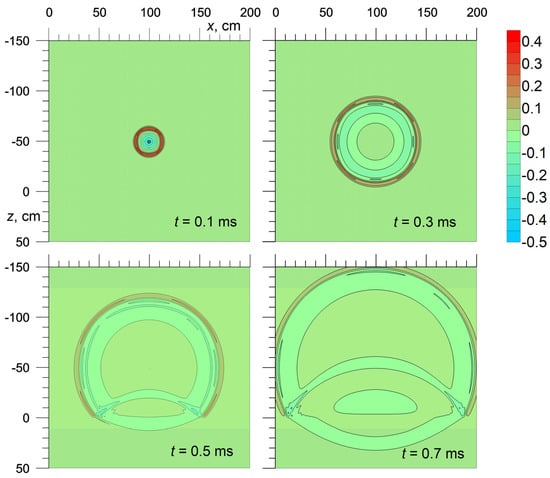
Figure 4.
The field of dimensionless pressure difference when the perturbation propagates from the source and passes/reflects through the boundary of two single-phase media for several time points. The color scale on the right shows a pressure level .
4.3. Propagation of the Perturbation from the Source and Passage/Reflection through the Boundary of a Porous Medium and Fractured-Porous Medium
Let us now consider the case of a layered and fractured porous medium. Let a porous medium border on another porous medium with the following fractures: area 1 (−1.5 m < z < 0, 0 < x < 2 m) is occupied by a porous medium, area 2 (0 < z < 0.5 m, 0 < x < 2 m) is occupied by a fractured porous medium. For both media, the skeleton material is quartz, the saturating liquid is water.
The characteristics of a porous medium are as follows: = 0.25, = 0.05 mm, = 6 GPa, = 50; parameters of a fractured porous medium are: = 0.29, = 0.01, = 0.05 mm, = 0.5 mm, = 148.5 mm, = 6 GPa, = 2 GPa, = 50, = 10; = 0.1.
At the boundary of the two media, the conditions of equality of the fluid flow, its pressure, and total stress are met. In the process of end-to-end computing, these conditions are fulfilled automatically. Fulfillment of continuity conditions at the boundaries of the layers was verified and confirmed by the output and verifying these quantities near the boundary nodes of the computational grid during the calculation process.
The source of the perturbation is located in a porous medium (area 1), and its location, size, and intensity are the same as in test 2.
Figure 5 shows the fields of dimensionless average pressure in the liquid (averaged by pores and fractures fluid pressure). When a perturbation propagates from a source in a porous medium, two compression zones are observed in the pressure field, which correspond to fast and slow waves (Figure 5, t = 0.1 and 0.2 ms). Then, the fast wave is reflected from the boundary and passes into the fractured porous medium (t = 0.3 and 0.4 ms). The slow wave in area 1 does not reach the border during this time. The interference of slow and reflected fast pressure waves is observed in area 1 (t = 0.3 and 0.4 ms).
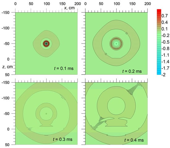
Figure 5.
The fields of average pressure in a liquid during the propagation of the perturbation from the source and its passage/reflection through the boundary of the porous media and fractured-porous media for several time points. The color scale on the right shows the pressure level .
As a test, the calculations of the propagation of the perturbation in one-dimensional and two-dimensional cases were compared (Figure 6). In the one-dimensional problem (a), the properties, location of the porous and fractured porous media, the position, and the characteristics of the perturbation source correspond to the line x = 100 cm for the two-dimensional problem (b). In Figure 6, in both cases, fast and slow wave modes propagating from the perturbation source in opposite directions are observed. At the boundary of the media at t = 0.2 ms, the formation of a wave passing into a fractured-porous medium and reflecting from it is visible. In the two-dimensional case, the amplitudes of the waves decrease significantly as they move away from the source, which is explained by their radial divergence.
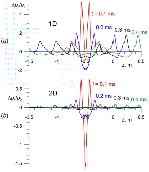
Figure 6.
The average pressure profiles in a liquid when a perturbation propagates from a source and passes/reflects through the boundary of the porous media and fractured-porous media for several time points in one-dimensional (a) and two-dimensional (b) cases, x = 100 cm.
Note that in a fractured porous medium, the wave contains three modes [10]. However, in these calculations, the third mode does not manifest itself due to the small amplitude and very fast attenuation.
5. Conclusions
A new approach to the numerical study of arbitrary waveform impulses in a layered porous and fractured-porous medium in a two-dimensional formulation has been developed. The possibility of using the finite-difference MacCormack method in relation to the problem of the propagation and passage of waves from a porous medium to a fractured porous medium in a two-dimensional formulation is shown. A computer implementation of the model and calculations is performed showing the effectiveness of the proposed methodology.
In this study, the problems of wave propagation in the case of a plane boundary between media were considered. The subsequent development of this approach will make it possible to calculate the propagation of disturbances in porous media with more complex zonal inhomogeneities.
Author Contributions
Conceptualization, A.A.G.; methodology, A.A.G., O.Y.B. and D.N.D.; software, O.Y.B.; investigation, A.A.G., O.Y.B. and D.N.D.; writing—original draft preparation, A.A.G., O.Y.B. and D.N.D. All authors have read and agreed to the published version of the manuscript.
Funding
The research was carried out within the state assignment of the Ministry of Science and Higher Education of the Russian Federation (project no. 121030500156-6).
Institutional Review Board Statement
Not applicable.
Informed Consent Statement
Not applicable.
Data Availability Statement
The data presented in this study are available upon request from the corresponding author.
Conflicts of Interest
The authors declare no conflict of interest.
References
- Khasanov, M.K.; Rafikova, G.R.; Musakaev, N.G. Mathematical Model of Carbon Dioxide Injection into a Porous Reservoir Saturated with Methane and its Gas Hydrate. Energies 2020, 13, 440. [Google Scholar] [CrossRef]
- Musakaev, N.G.; Khasanov, M.K. Solution of the Problem of Natural Gas Storages Creating in Gas Hydrate State in Porous Reservoirs. Mathematics 2020, 8, 36. [Google Scholar] [CrossRef]
- Gubaidullin, A.A.; Boldyreva, O.Y. Waves in a porous medium with a gas hydrate containing layer. J. Appl. Mech. Tech. Phys. 2020, 61, 525–531. [Google Scholar] [CrossRef]
- Kutushev, A.G.; Rudakov, D.A. Numerical study of the impact of a shock wave on an obstacle shielded by a layer of porous powdery medium. J. Appl. Mech. Tech. Phys. 1993, 34, 25–31. (In Russian) [Google Scholar]
- Zhilin, A.A.; Fedorov, A.V. Applying the TVD scheme to calculate two-phase flows with different velocities and pressures of the components. Math. Model. Comput. Simul. 2008, 20, 72–87. [Google Scholar] [CrossRef]
- Lax, P.D.; Wendroff, B. Systems of conservation laws. Commun. Pure Appl. Math. 1960, 13, 217–237. [Google Scholar] [CrossRef]
- Gubaidullin, A.A.; Dudko, D.N.; Urmancheev, S.F. Influence of air shock waves on obstacles covered by porous layer. Comput. Technol. 2001, 6, 7–20. (In Russian) [Google Scholar]
- Gubaidullin, A.A.; Boldyreva, O.Y.; Dudko, D.N. Elastic waves in a porous medium with layers of different permeabilities. Lobachevskii J. Math. 2021, 42, 1977–1981. [Google Scholar] [CrossRef]
- Tuncay, K.; Corapcioglu, M.Y. Wave propagation in fractured porous media. Transp. Porous Media 1996, 23, 237–258. [Google Scholar] [CrossRef]
- Gubaidullin, A.A.; Kuchugurina, O.Y. Propagation of weak perturbations in cracked porous media. J. Appl. Math. Mech. 1999, 63, 769–777. [Google Scholar] [CrossRef]
- Nigmatulin, R.I. Dynamics of Multiphase Media; Part 1; Hemisphere Publisher: New York, NY, USA, 1990. [Google Scholar]
- Barenblatt, G.I.; Zheltov, Y.P.; Kochina, I.N. Basic concepts in the theory of seepage of homogeneous liquids in fissured rocks. J. Appl. Math. Mech. 1960, 24, 1286–1303. [Google Scholar] [CrossRef]
- MacCormack, R.W. The effect of viscosity in hypervelocity impact cratering. AIAA Pap. 1969, 69, 354–361. [Google Scholar]
- Deresiewicz, H.; Skalak, R. On uniqueness in dynamic poroelasticity. Bull. Seismol. Soc. Am. 1963, 53, 783–788. [Google Scholar] [CrossRef]
- Wang, Y.-F.; Liang, J.-W.; Chen, A.-L.; Wang, Y.-S.; Laude, V. Wave propagation in one-dimensional fluid-saturated porous metamaterials. Phys. Rev. B 2019, 99, 134304. [Google Scholar] [CrossRef]
- Zhang, S.-Y.; Yan, D.-J.; Wang, Y.-S.; Wang, Y.-F.; Laude, V. Wave propagation in one-dimensional fluid-saturated porous phononic crystals with partial-open pore interfaces. Int. J. Mech. Sci. 2021, 195, 106227. [Google Scholar] [CrossRef]


Disclaimer/Publisher’s Note: The statements, opinions and data contained in all publications are solely those of the individual author(s) and contributor(s) and not of MDPI and/or the editor(s). MDPI and/or the editor(s) disclaim responsibility for any injury to people or property resulting from any ideas, methods, instructions or products referred to in the content. |
© 2023 by the authors. Licensee MDPI, Basel, Switzerland. This article is an open access article distributed under the terms and conditions of the Creative Commons Attribution (CC BY) license (https://creativecommons.org/licenses/by/4.0/).