A Machine Learning Approach to Detect Parkinson’s Disease by Looking at Gait Alterations

Abstract

Parkinson’s disease (PD) is often detected only in later stages, when about 50% of nigrostriatal dopaminergic projections have already been lost. Thus, there is a need for biomarkers to monitor the earliest phases, especially for those that are at higher risk. In this work, we explore the use of machine learning methods to diagnose PD by analyzing gait alterations via an inertial sensors system that participants in the study wear while walking down a 15 m long corridor in three different scenarios. To achieve this goal, we have trained six well-known machine learning models: support vector machines, logistic regression, neural networks, k nearest neighbors, decision trees and random forest. We thoroughly explored several ways to mitigate the problems derived from the small amount of available data. We found that, while achieving accuracy rates of over 70% is quite common, the accuracy of the best model trained is only slightly above the 80% mark. This model has high precision and specificity (over 90%), but lower sensitivity (only 71%). We believe that these results are promising, especially given the size of the population sample (41 PD patients and 36 healthy controls), and that this research venue should be further explored.

1. Introduction

Parkinson’s disease (PD) is a disorder of the central nervous system that progressively alter the body’s motor capacities. Symptoms present insidiously, in the form of tremor or clumsiness or slowness of movement. In early stages of the disease, the patient’s facial expression may not show any signs. While the disease progresses, speech may be altered, as well as the movement of arms while walking. Other serious problems such as dementia and difficulties thinking, eating or sleeping or issues such as depression may appear, although in more advanced stages. PD cannot be cured, but medical treatment may improve the symptoms. Moreover, some specific medications (such as L-dopa or dopamine agonists) are more effective when administered early on. Unfortunately, many patients are diagnosed only when the disease is more advanced and symptoms are visible.

This is precisely why clinicians and researchers have directed their efforts into finding medical biomarkers that are specific to PD and could be easily detected early on (see [1] for a thorough survey). In particular, there are many works based on gait study that demonstrate that sensitive sensor measurements may show some disorder in the motor system. Mirelman et al. [2] mention that gait impairments are related to neural connectivity and structural network topology, and thus, are important for diagnosing PD. Pistacchi et al. [3] have observed a difference in gait measurements for PD patients compared with healthy controls in cadence, stride duration, stance duration, swing phase and swing duration, step width, stride length and swing velocity. Moris et al. [4] study gait alterations for patients with and without medication. They observed gait changes in PD patients such as a lower amplitude of movement in the legs’ joints (in all directions). Lewek et al. [5] state that observing an asymmetry of arm swing may be useful for early diagnosis of PD and, thus, for tracking disease progression in patients with later PD. Baltadjieva et al. [6] detected a modified gait pattern in “de novo” PD, although dramatic changes in the gait pattern were not yet visible (“de novo” refers to an individual that does not take prescribed PD-specific medications yet).

So, we know that PD patients show gait alteration even in the early stages. By the time other symptoms appear (roughly 5 to 20 years after the disease has taken over the brain), more than 50% of neural cells that produce dopamine have already died. The question is: can we detect these gait disturbances just by “looking” at how they walk? In the affirmative case, people that are at higher risk (for example, those that have diagnosed cases among relatives or those with the G2019S mutation in the LRRK2 gene, who have a 50% probability to develop the disease at some point in life) could be periodically monitored. In this study, we address this issue by devising a two-step process: we first extract gait parameters from the information provided by an inertial sensors system attached to fixed positions on the body, and then we use these parameters to train a machine learning model to distinguish between PD patients and healthy controls.

Note that the vast majority of studies that use spatial–temporal gait features (for PD detection or elsewhere) employ Kinect systems [7,8,9,10], but other motion caption detectors also exist. For example, in [11], an 8-camera video motion analysis system measured reflective marker positions, while GRFs (ground reaction forces) were recorded simultaneously using two instrumented force platforms. The vertical GRF of the 16 sensors located under the feet of each participant was also used to build the PhysioNet dataset [12], on which research in [13,14] is based. Fewer studies use inertial sensors only (for example, in [15], each participant wore a device located on the area of the fourth and fifth lumbar vertebrae), and information is drawn mainly from accelerometer values, not from joint angles, as we did. The procedure of measuring angles to characterize the human motion also appears in [16,17], where the authors used it for the movement of both human and robots. However, in these last two references, the methodology of simulating human motion is different. It is based on non-linear mathematical tools and also on expensive hardware (in particular, on the Perception Neuron Studio, featuring professional motion capture hardware for production in biomechanics). The key element is the calculation of motion mass parameters, which are able to describe the amount and smoothness of movements, also used in [8,18].

The range of walking scenarios in the studies that pursue the identification of PD patients from gait alterations is quite wide: in [19], PD patients walked a 200 m corridor at their preferred pace; in [20], they were instructed to walk for 5 min in a 77 m long hallway; in [15], participants traversed a 20 m walkway under four different conditions, while in [11], subjects walked at their preferred walking speed ten times across an 8 m walkway. Note that shorter distances, such as the one employed in the Timed-Up-and-Go (TUG) test (in combination with a Kinect system), proved to be sufficient for the calculation of motion mass parameters in [8,18].

Reported accuracy values for the existing systems are in the 70–95% range, depending mainly on the motion capture hardware used, the mathematical tools employed or the machine learning models applied. Some examples include values between 75% and 85% in [8], 86.75% in [13], between 80.4% and 92.6% in [11], 76% in [19], 92.7% in [14] and 90% in [20]. In the present study, we show the extent to which angles measured by an inertial sensor system can be useful in detecting PD with a relatively small cohort of participants.

The remainder of the article is structured as follows. In Section 2 we explain the characteristics of the study population (Section 2.1), the variables extracted from the inertial sensors (Section 2.2), the predictors used and their acquisition process (Section 2.3). We apply dimensionality reduction techniques (in Section 2.4) to visualize the data we work with, and we present the machine learning models employed (Section 2.5), and the evaluation metrics that allow us to compare their performance (Section 2.6). In Section 3, we first exhibit the error rates obtained when training and testing these models on the original dataset. Since these preliminary results indicate that our models are overfitting the training data, and therefore fail to generalize well to unseen examples, we address this issue in the next subsections by applying the typical overfitting mitigation techniques: feature selection (Section 3.1), regularization (Section 3.2), increasing the size of the dataset (Section 3.3) and fine-tuning meta-parameters (Section 3.4). Finally, we show the performance (in terms of error rates) of those models that perform best in their respective class (Section 3.5). In Section 4 we discuss other performance indicators for the model that achieved the best accuracy value. Concluding remarks are presented in Section 5.

2. Materials and Methods

The study population consisted of 41 PD patients (20 patients with LRRK2 G2019S mutation and 21 idiopathic PD patients) and 36 healthy controls (HCs), 17 of them being non-carrier relatives of LRRK2 patients (the rest were unrelated controls, mostly spouses of PD patients). According to [21], idiopathic PD refers to “the presence of signs and symptoms of PD for which the etiology is currently unknown and in which there is no known family history of PD”. The average age of patients in the PD group is 67 ± 12.1 years, their mean disease duration is 6.2 ± 3.9 years and their UPDRS-III (Unified Parkinson’s disease rating scale) score is 29.9 ± 14.9. Participants in the HC group had a mean age of 64 ± 10.1 years. We refer the reader to (page 23, Table 1) [22] for more detailed statistics on other anthropomorphic parameters and MoCA (Montreal Cognitive Assessment) scores.

2.1. Procedures

Each of the participants took part in three different experiments, in which they were asked to walk along a 15 m-long, well-lit corridor, turning as many times as needed. In the first one (usual walk), the subject has to walk for one minute at a normal walking pace. In the second experiment (fast walk), the subject is asked to walk those 15 m as fast as possible (with no turns this time). In the last experiment (dual task), the subject has to walk for one minute while skip counting backwards by threes, beginning with 100 (again, the participant has to turn each time the 15 m corridor is entirely covered).

The subjects are equipped with a total of 16 lightweight sensors (STT-IWS, STT Systems, San Sebastian, Spain), distributed over the body as shown in Figure 1: forehead (1), torso (1), shoulders (2), elbows (2), wrists (2), hips (2), knees (2), ankles (2), cervix (1) and pelvis (1). The sensors are synchronized and precalibrated, referencing the vertical axis in the anatomical position, and they provide discrete information (every 0.01 of a second) about the angles of each segment with respect to its original position.

2.2. Variables

Although the raw information received from the sensors is in the form of quaternions, the software used for these experiments already transforms it into angles. Thus, we could use the information provided by a total of 42 variables as described in

Table 1. Number of angles measured by the 16 sensors.

	Ankles	Knees	Hips	Wrists	Elbows	Shoulders	Cervix	Pelvis	Torso
Flexion-extension-	-	2	2	2	2	2	1	-	1
Abduction-adduction	-	2	2	2	-	2	-	-	-
Rotation	2	2	2	2	-	2	1	1	1
Lateral flexion	-	-	-	-	-	-	1	-	1
Tilt	-	-	-	-	-	-	-	1	1
Obliquity	-	-	-	-	-	-	-	1	-
Eversion-inversion	2	-	-	-	-	-	-	-	-
Dorsi/plantar flexion	2	-	-	-	-	-	-	-	-
Total	6	6	6	6	2	6	3	3	4

.

Additionally, the time instances in which each foot touches the floor and takes off are also separately stored in a text file called Events (we shall refer to this file again in Appendix A). This information will serve to identify the actual steps.

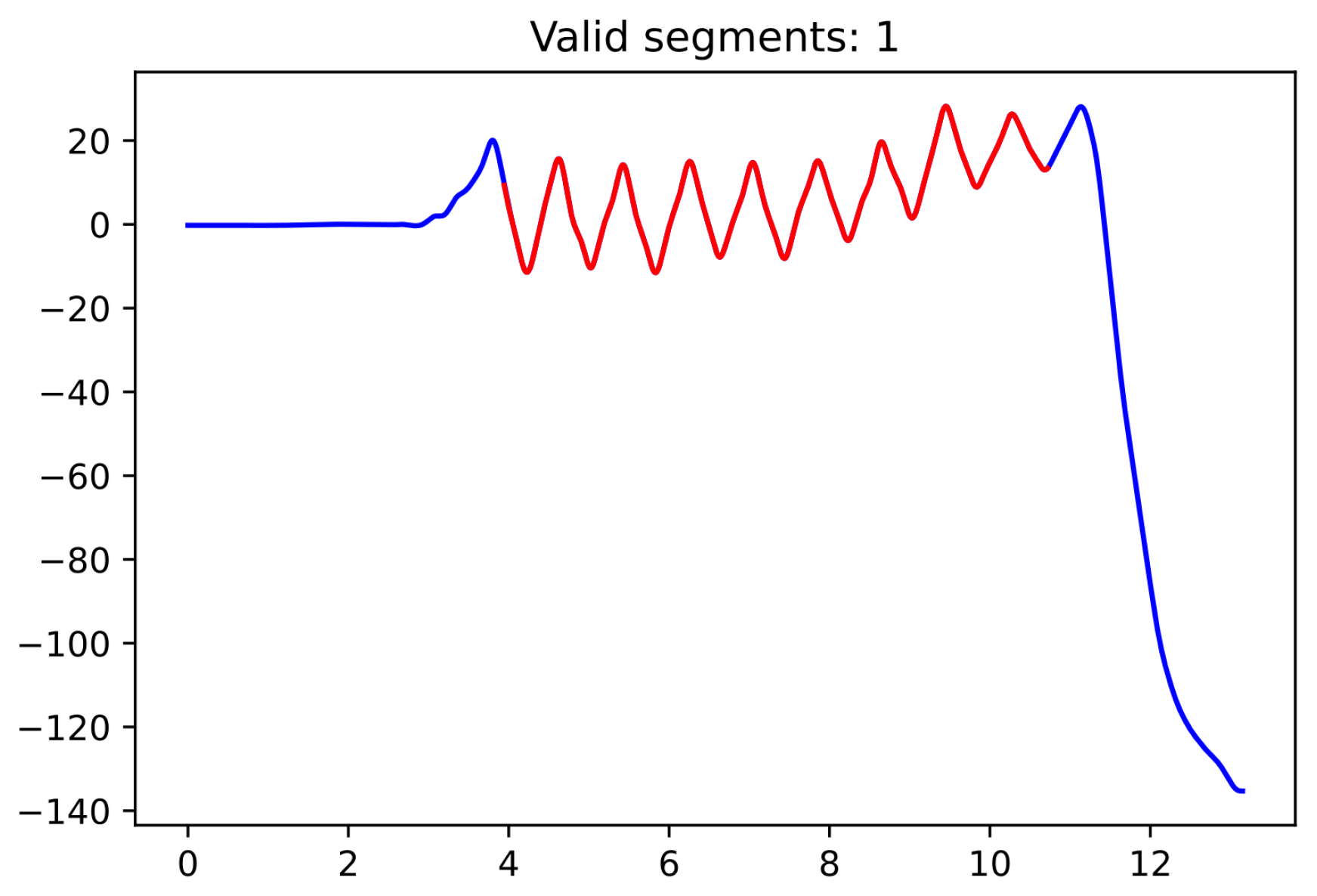
Since the moment in which the subject is turning is not specifically recorded as such, we used the pelvic rotation angle (see Figure 2) to help us identify those segments of straight-line walking (for technical details, see Appendix A). Abnormal segments or those that do not have enough steps (specifically, at least 15 steps are required since the corridor’s total length is 15 m) were discarded.

2.3. Predictors

Once the segments are identified, the next step is the extraction of various measures (called predictors) that could help distinguish between individuals of different groups (for each participant and each of the three experiments). In particular, refs. [23,24,25] show that gait disturbances and reduced arm swing are often observed early in the course of the disease.

For each subject and each of the three experiments (usual walk, fast walk and dual task), we computed the following measures:

• Gait speed (m/s) was calculated as the ratio between the distance walked (15 m) and the ambulation time.
• Step time (s) was determined as the time elapsed between the foot’s takeoff and initial contact of the same foot (the mean, standard deviation and variability are calculated over all steps of the experiment; the first and last steps in each segment were discarded; the variability of a variable is computed as the ratio between its standard deviation and its mean, multiplied by 100). The left and right foot step times were also recorded, as studies showed more acute differences between values (mean and variability) of the dominant and the non-dominant foot in PD patients [26]. For the same reason, asymmetry was also calculated (to obtain the asymmetry of a variable, one has to divide by 90° the difference between 45° and the arctangent of the ratio of greatest to smallest values and then multiply it by 100).
• Stride time (s): is computed as the time elapsed between two consecutive initial contacts of a given foot. The same measures (mean, standard deviation and variability) as in the case of the step time were recorded, without looking into differences between the right and left foot (no steps discarded this time to maximize the number of strides).
• Step length (m) was calculated by dividing the length of the corridor (15 m) by the number of steps identified in that segment (no steps discarded in this case). The mean was computed as the average over all segments (since the fast-walking experiment only has one segment, computing standard deviation in this case makes no sense).
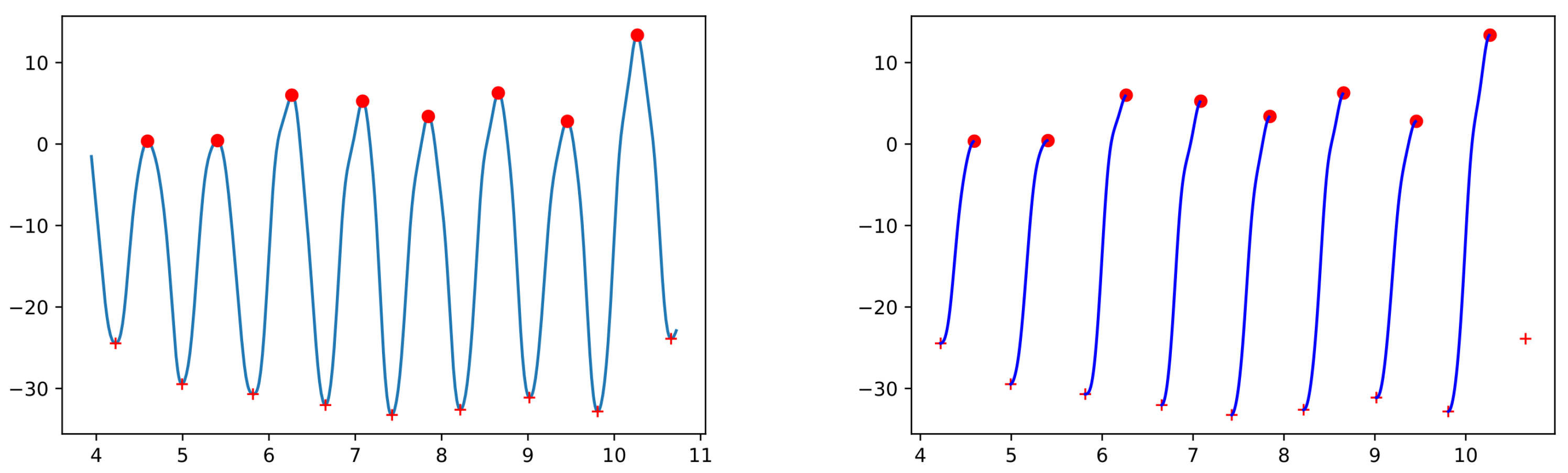
• Hip amplitude (deg) is computed (using the hip’s flexion–extension values while walking) as the range from peak flexion to peak extension (see Appendix C for a more detailed explanation). We record the overall mean, standard deviation, variability and asymmetry over all segments in the experiment and also the mean and variability for each individual leg.
• Left and right arm amplitude (deg) is computed as the range from peak flexion to peak extension (using the shoulder’s flexion–extension values). The mean, jerk and variability values for each arm are recorded. The jerk is a measure of the smoothness of the movement and the literature contains several ways of computing it—see [27] for a survey. We chose to compute the mean absolute jerk normalized by peak speed introduced in [28] (check Appendix C for details on how to compute it). The overall mean, standard deviation, variability and asymmetry are also computed.
• Left and right elbow amplitude (deg) is computed as the range from peak flexion to peak extension (using the elbow’s flexion–extension values). The mean and variability values for each arm are recorded. The overall mean, standard deviation, variability and asymmetry are also computed.
• The trunk rotation amplitude (deg) is computed using the torso’s rotation angle between its minimum and maximum values within one step (left or right step, respectively). The overall mean is recorded and the values corresponding to the left and right steps are used to compute the asymmetry. Finally, the mean absolute jerk normalized by peak speed is computed without taking into account the side.

Note that, for participants in the HC group, the dominant side was taken to be the one of preferential use. In the name of the predictors, AND refers to “Affected or non-dominant side” and NAD refers to “Not affected or dominant side”.

Apart from the 3 × 42 predictors mentioned above and detailed in

Table A1. Trunk-related predictors (mean and SD values, shown as mean ± SD).

Name of Predictor	Experiment	PDs ($\mathit{n}=41$)	HCs ($\mathit{n}=36$)	Description
	Usual walk	$10.72\pm 4.74$	$12.54\pm 4.60$
TrunkRotationAmplitude	Fast walk	$14.73\pm 6.48$	$15.63\pm 6.06$	Trunk rotation amplitude, deg
	Dual task	$10.56\pm 4.82$	$12.67\pm 4.11$
	Usual walk	$-4.41\pm 4.16$	$-3.26\pm 2.26$
TrunkRotationAsymmetry	Fast walk	$-4.31\pm 4.29$	$-6.08\pm 7.20$	Trunk rotation asymetry, %
	Dual task	$-4.95\pm 3.77$	$-3.95\pm 2.90$
	Usual walk	$8168.33\pm 2013.61$	$7733.02\pm 1586.73$
TrunkJerk	Fast walk	$8149.42\pm 2287.85$	$8409.24\pm 1910.06$	Trunk jerk, m/s3
	Dual task	$8138.22\pm 2088.13$	$7615.75\pm 1469.47$

,

Table A2. Walk-related predictors (mean and SD values, shown as mean ± SD).

Name of the Predictor	Experiment	PDs $(\mathit{n}=41)$	HCs $(\mathit{n}=36)$	Description
	Usual walk	$1.23\pm 0.23$	$1.41\pm 0.18$
Speed	Fast walk	$1.62\pm 0.39$	$1.91\pm 0.33$	Gait speed, m/s
	Dual task	$1.18\pm 0.24$	$1.40\pm 0.18$
	Usual walk	$0.64\pm 0.11$	$0.72\pm 0.07$
StepLengthMean	Fast walk	$0.73\pm 0.15$	$0.81\pm 0.10$	Step length mean, m
	Dual task	$0.63\pm 0.12$	$0.71\pm 0.07$
	Usual walk	$0.45\pm 0.05$	$0.44\pm 0.04$
StepTimeMean	Fast walk	$0.39\pm 0.05$	$0.36\pm 0.05$	Step time mean, s
	Dual task	$0.47\pm 0.05$	$0.44\pm 0.04$
	Usual walk	$0.05\pm 0.04$	$0.03\pm 0.02$
StepTimeStd	Fast walk	$0.04\pm 0.03$	$0.05\pm 0.05$	Step time standard deviation, s
	Dual task	$0.05\pm 0.03$	$0.04\pm 0.03$
	Usual walk	$11.04\pm 8.96$	$7.91\pm 5.53$
StepTimeVariability	Fast walk	$10.59\pm 11.24$	$16.41\pm 17.12$	Step time variability, %
	Dual task	$10.54\pm 6.86$	$8.98\pm 7.60$
	Usual walk	$-5.52\pm 5.22$	$-3.50\pm 2.95$
StepTimeAsymmetry	Fast walk	$-4.70\pm 5.50$	$-6.93\pm 8.25$	Step time asymmetry, %
	Dual task	$-4.71\pm 3.71$	$-4.11\pm 4.06$
	Usual walk	$1.06\pm 0.09$	$1.03\pm 0.09$
StrideTimeMean	Fast walk	$0.91\pm 0.09$	$0.86\pm 0.09$	Stride time mean, s
	Dual task	$1.08\pm 0.11$	$1.03\pm 0.08$
	Usual walk	$0.06\pm 0.10$	$0.03\pm 0.02$
StrideTimeStd	Fast walk	$0.04\pm 0.03$	$0.05\pm 0.04$	Stride time standard deviation, s
	Dual task	$0.06\pm 0.06$	$0.04\pm 0.04$
	Usual walk	$5.64\pm 9.03$	$3.02\pm 1.95$
StrideTimeVariability	Fast walk	$4.02\pm 3.59$	$5.39\pm 4.91$	Stride time variability, %
	Dual task	$5.25\pm 5.14$	$4.09\pm 4.26$
	Usual walk	$32.73\pm 6.18$	$35.93\pm 5.34$
HipAmplMean	Fast walk	$37.90\pm 7.51$	$41.48\pm 5.91$	Hip amplitude mean, deg
	Dual task	$33.37\pm 6.23$	$37.05\pm 5.30$
	Usual walk	$3.63\pm 2.26$	$3.84\pm 2.70$
HipAmplStd	Fast walk	$3.24\pm 1.82$	$3.94\pm 3.16$	Hip amplitude standard deviation, deg
	Dual task	$3.63\pm 2.61$	$3.53\pm 2.60$
	Usual walk	$11.59\pm 7.61$	$11.49\pm 10.01$
HipAmplVariability	Fast walk	$8.90\pm 5.13$	$10.06\pm 9.58$	Hip amplitude variability, %
	Dual task	$10.95\pm 7.27$	$10.08\pm 8.77$
	Usual walk	$-5.91\pm 4.25$	$-6.15\pm 5.16$
HipAmplAsymmetry	Fast walk	$-4.56\pm 3.55$	$-5.27\pm 4.21$	Hip amplitude asymmetry, %
	Dual task	$-5.33\pm 4.04$	$-5.21\pm 4.51$
	Usual walk	$0.46\pm 0.07$	$0.43\pm 0.05$
AND_StepTimeMean	Fast walk	$0.38\pm 0.06$	$0.33\pm 0.08$	AND step time mean, s
	Dual task	$0.46\pm 0.07$	$0.43\pm 0.06$
	Usual walk	$0.45\pm 0.07$	$0.45\pm 0.05$
NAD_StepTimeMean	Fast walk	$0.39\pm 0.06$	$0.39\pm 0.05$	NAD step time mean, s
	Dual task	$0.47\pm 0.07$	$0.46\pm 0.05$
	Usual walk	$6.28\pm 6.55$	$5.66\pm 5.85$
AND_StepTimeVariability	Fast walk	$7.77\pm 11.43$	$15.71\pm 21.36$	AND step time variability, %
	Dual task	$7.38\pm 7.03$	$6.80\pm 8.74$
	Usual walk	$6.09\pm 4.77$	$4.66\pm 2.65$
NAD_StepTimeVariability	Fast walk	$5.51\pm 7.25$	$8.17\pm 8.90$	NAD step time variability, %
	Dual task	$6.60\pm 4.24$	$4.40\pm 2.05$
	Usual walk	$32.23\pm 6.68$	$34.21\pm 7.52$
AND_HipAmplMean	Fast walk	$37.34\pm 7.98$	$39.95\pm 7.89$	AND hip amplitude mean, deg
	Dual task	$32.51\pm 6.30$	$35.65\pm 7.41$
	Usual walk	$33.34\pm 7.61$	$37.93\pm 5.01$
NAD_HipAmplMean	Fast walk	$38.50\pm 8.44$	$43.33\pm 5.83$	NAD hip amplitude mean, deg
	Dual task	$34.35\pm 7.93$	$38.65\pm 4.86$
	Usual walk	$5.92\pm 7.12$	$6.00\pm 10.54$
AND_HipAmplVariability	Fast walk	$4.26\pm 2.10$	$5.43\pm 12.49$	AND hip amplitude variability, %
	Dual task	$6.98\pm 7.16$	$5.53\pm 9.95$
	Usual walk	$5.35\pm 3.45$	$3.59\pm 1.08$
NAD_HipAmplVariability	Fast walk	$4.06\pm 2.04$	$3.17\pm 1.53$	NAD hip amplitude variability, %
	Dual task	$5.05\pm 2.54$	$3.56\pm 1.63$

and

Table A3. Arm-related predictors (mean and SD values, shown as mean ± SD).

Name of Predictor	Experiment	PDs ($\mathit{n}=41$)	HCs ($\mathit{n}=36$)	Description
	Usual walk	$9.26\pm 7.50$	$16.33\pm 9.64$
AND_ArmAmplMean	Fast walk	$15.06\pm 12.32$	$25.40\pm 11.95$	AND arm swing amplitude mean, deg
	Dual task	$10.87\pm 9.87$	$22.02\pm 10.60$
	Usual walk	$12.10\pm 6.67$	$16.46\pm 10.61$
NAD_ArmAmplMean	Fast walk	$20.09\pm 10.94$	$23.84\pm 13.29$	NAD arm swing amplitude mean, deg
	Dual task	$15.20\pm 8.66$	$19.89\pm 11.76$
	Usual walk	$37.03\pm 17.55$	$27.78\pm 16.82$
AND_ArmAmplVariability	Fast walk	$27.06\pm 19.46$	$15.27\pm 10.65$	AND arm swing variability, %
	Dual task	$37.67\pm 20.07$	$26.71\pm 17.90$
	Usual walk	$32.24\pm 18.35$	$29.14\pm 20.08$
NAD_ArmAmplVariability	Fast walk	$22.38\pm 20.67$	$19.66\pm 18.37$	NAD arm swing variability, %
	Dual task	$33.55\pm 23.13$	$31.94\pm 22.39$
	Usual walk	$9064.17\pm 4323.18$	$6906.23\pm 2565.76$
AND_ArmJerk	Fast walk	$9559.72\pm 5171.12$	$8111.88\pm 3283.50$	AND arm jerk, m/s3
	Dual task	$9505.10\pm 5293.61$	$6565.00\pm 2194.89$
	Usual walk	$6905.75\pm 1982.91$	$6722.09\pm 2280.84$
NAD_ArmJerk	Fast walk	$7150.47\pm 2257.58$	$8158.46\pm 2696.66$	NAD arm jerk, m/s3
	Dual task	$6627.30\pm 2437.04$	$6608.49\pm 2271.82$
	Usual walk	$9.98\pm 6.26$	$20.20\pm 11.34$
AND_ElbowAmplMean	Fast walk	$18.00\pm 14.20$	$31.84\pm 14.07$	AND elbow amplitude mean, deg
	Dual task	$10.64\pm 8.02$	$25.30\pm 11.64$
	Usual walk	$12.56\pm 7.25$	$17.56\pm 11.20$
NAD_ElbowAmplMean	Fast walk	$21.53\pm 12.44$	$26.33\pm 15.34$	NAD elbow amplitude mean, deg
	Dual task	$14.27\pm 7.99$	$19.60\pm 10.90$
	Usual walk	$38.24\pm 17.41$	$33.88\pm 20.54$
AND_ElbowAmplVariability	Fast walk	$31.99\pm 21.35$	$24.26\pm 20.90$	AND elbow amplitude variability, %
	Dual task	$47.30\pm 18.20$	$38.09\pm 24.38$
	Usual walk	$39.96\pm 22.78$	$34.63\pm 18.27$
NAD_ElbowAmplVariability	Fast walk	$31.42\pm 23.80$	$32.75\pm 27.30$	NAD elbow amplitude variability, %
	Dual task	$46.03\pm 22.50$	$48.80\pm 26.04$
	Usual walk	$9.96\pm 5.39$	$16.03\pm 9.24$
ArmAmplMean	Fast walk	$16.87\pm 10.19$	$24.23\pm 11.67$	Arm amplitude mean, deg
	Dual task	$11.95\pm 7.71$	$20.33\pm 9.73$
	Usual walk	$5.17\pm 2.76$	$5.17\pm 2.79$
ArmAmplStd	Fast walk	$6.19\pm 3.52$	$5.77\pm 3.16$	Arm amplitude standard deviation, deg
	Dual task	$6.34\pm 3.57$	$7.33\pm 4.00$
	Usual walk	$57.71\pm 26.48$	$38.25\pm 20.16$
ArmAmplVariability	Fast walk	$45.95\pm 28.93$	$28.97\pm 19.66$	Arm amplitude variability, %
	Dual task	$63.52\pm 32.74$	$42.45\pm 25.79$
	Usual walk	$-21.65\pm 12.34$	$-12.66\pm 9.95$
ArmAmplAsymmetry	Fast walk	$-17.98\pm 12.11$	$-11.38\pm 10.09$	Arm amplitude variability, %
	Dual task	$-23.01\pm 14.51$	$-15.21\pm 12.27$
	Usual walk	$10.65\pm 5.37$	$18.66\pm 10.47$
ElbowAmplMean	Fast walk	$18.62\pm 11.02$	$28.29\pm 12.56$	Elbow amplitude mean, %
	Dual task	$11.65\pm 5.88$	$21.95\pm 9.72$
	Usual walk	$5.62\pm 2.16$	$7.10\pm 4.90$
ElbowAmplStd	Fast walk	$8.50\pm 4.48$	$10.28\pm 6.79$	Elbow amplitude standard deviation, deg
	Dual task	$7.40\pm 3.16$	$10.54\pm 5.92$
	Usual walk	$59.96\pm 25.49$	$41.70\pm 18.16$
ElbowAmplVariability	Fast walk	$55.28\pm 27.83$	$40.43\pm 26.01$	Elbow amplitude variability, %
	Dual task	$68.67\pm 22.51$	$51.50\pm 24.16$
	Usual walk	$-20.57\pm 11.47$	$-11.11\pm 8.38$
ElbowAmplAsymmetry	Fast walk	$-20.97\pm 12.89$	$-13.23\pm 9.95$	Elbow amplitude asymmetry, deg
	Dual task	$-22.68\pm 11.32$	$-11.70\pm 9.70$

from Appendix B, we also used the age and the average turning time as predictors (the values are extracted from the first and third experiment, since in the second one, the participant only walks the corridor once, without turning around) in the previous study [22]. We decided to drop them here so as to only keep predictors specific to the three experiments (age was not one of these), which are present in all of them (the second experiment had no “turning time”).

2.4. Data Visualization

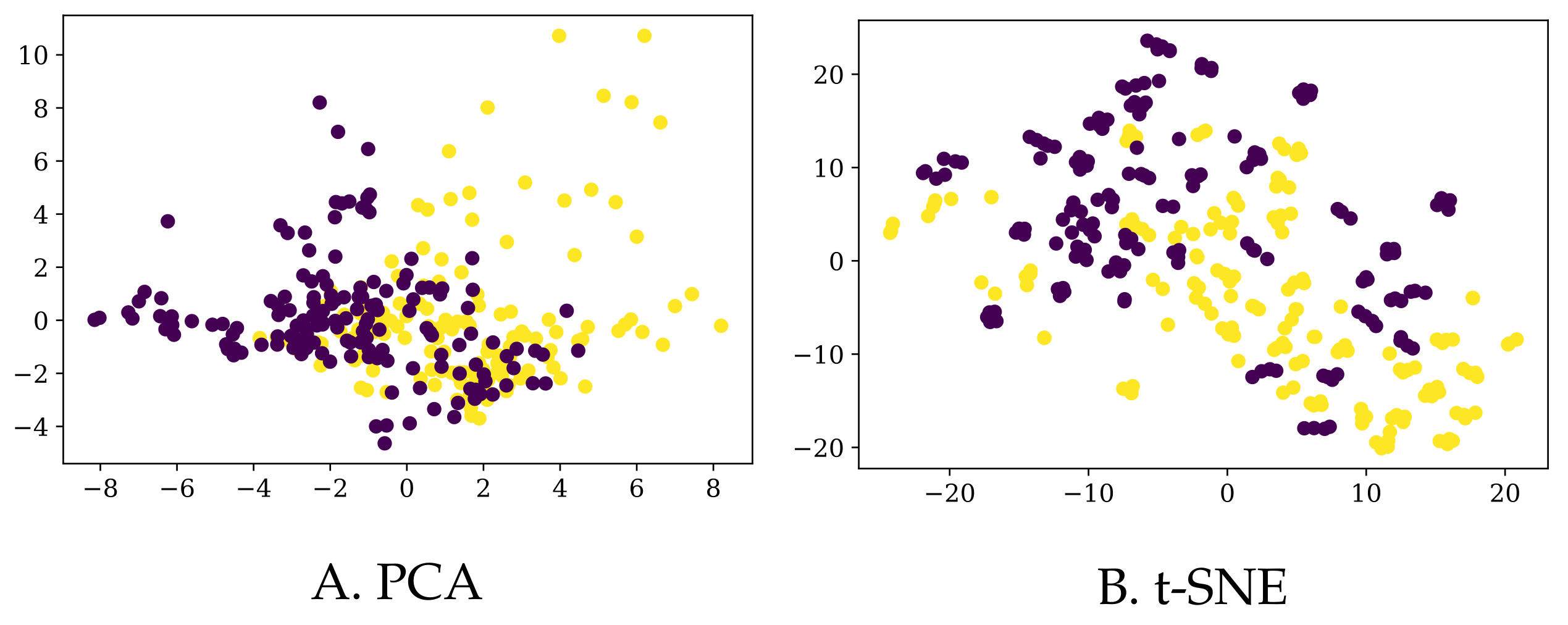
Since the information we have for each of the participants lies in a high-dimensional space, the only option to visualize the data in 2D or 3D maps is via dimensionality reduction algorithms. In particular, we used the t-distributed Stochastic Neighbor Embedding (t-SNE) [29] method and Principal Component Analysis (PCA) [30] to plot our data in 2D, as depicted in Figure 3. Of course, prior to applying any algorithm, we normalized all the columns to have a zero mean and a standard deviation of one.

First of all, let us note that based on the whole set of 126 predictors, it is not easy to separate the PD patients from the control group. Although this does not necessarily mean that they are not separable in higher dimension, it is an early indication that classifying these participants into their corresponding classes would not be easy. Additionally, the explained variance ratio of the first two components in the PCA reduction is rather low (0.19 and 0.11, respectively), so we should take this representation with caution.

Secondly, one could opt to select only those predictors that were shown to be relevant in [22]: “PD patients and controls showed differences in speed, stride length and arm swing amplitude, variability and asymmetry in all three tasks. […] Also, in fast walking and dual task situation, PD patients showed greater step and stride time”. Nonetheless, the 2D representations of this reduced dataset (only 19 columns) are similar to the ones displayed in Figure 3, so we chose not to include a dedicated figure here.

Finally, we also augmented the existing data in two different ways (details in Section 3.3), resulting in a bigger dataset (to which we refer as BigD) and a somewhat smaller one (yet still bigger than the original one as to the number of rows) called MedD. We plot their 2D representations (again, using PCA and tSNE) in Figure 4 and Figure 5, respectively.

Note that, although most of the times the entries corresponding to one participant are grouped together in the t-SNE 2D representation for the BigD dataset, they are more scattered in the case of PCA (for the same dataset), and even more so for the MedD dataset (although, admittedly, t-SNE still groups the entries of the same participant more than the PCA). In Figure 6 we show one example in which the entries corresponding to one participant are not close to each other.

By simply “glancing” at the data (via dimensionality reduction), it seems that obtaining more data does not make the task of identifying PD patients much easier (we will see in Section 3.3 that this is indeed the case).

2.5. Machine Learning Methods

We have handpicked six very well-known machine learning models to work with, aiming to cover a variety of different classification approaches. Apart from the four models described as “fundamental algorithms” in “The Hundred-Page Machine Learning Book” [31]: logistic regression (LR), support vector machines (SVMs), k Nearest Neighbors (kNN) and decision trees (DTs), we also included an ensemble method: Random Forest (RF), and the now famous artificial neural networks (NN), in their most basic form: Multilayer Perceptron (also thoroughly described in [31]). The size of the available data made us discard other, more complex models. We refer the reader to the above-mentioned book (or any other introductory book, for that matter) for details about how each of these models work.

2.6. Evaluation Metrics

The most common evaluation metric for the performance of a classification algorithm is the accuracy (defined as the ratio between the number of data points that are correctly predicted and the total number of examples analyzed). The error rate is the exact opposite: the number of misclassified examples out of all the data points (error rate + accuracy rate = 1). There are many other indicators that evaluate the performance of a model: the ROC curve and its AUC, sensitivity (also called recall), specificity, precision, 95-confidence interval and the confusion matrix. However, sometimes maximizing one indicator leads to smaller values of the others. So, our goal in this study is to maximize accuracy (which is the same as minimizing the error rate), and, once the best model is selected, we will report on all these other metrics.

Measuring the accuracy of the model on the same dataset used for training only gives us an overoptimistic estimate of the performance of the model on unseen data, so it is only useful for diagnostic purposes (here, the term is not used with its medical meaning; in machine learning, placing a diagnostic on a model implies understanding if the model under study is adequate—for example, if it avoids underfitting or overfitting the data). So, keeping a separate set for testing is a must. The size of this set will also influence the output: if too small, there is a high chance of choosing mostly “difficult” (or just the opposite, only “easy” examples). If the set is too big, there are too few data left with which to train the model. The recommended method is to perform n-fold cross-validation (typical values for n are 5 or 10), whereas its extreme version (Leave One Out cross validation), in which n is taken to be the total number of points in the dataset, is only possible if the size of the dataset is small enough (as in our case).

So, apart from the above-mentioned Leave One Out (LOO) cross-validation evaluation method, in this study we have randomly selected 65% of the data for training (50 entries), and the rest of 35% (27 entries) was reserved for the test set. We made sure that the percentage of PD patients is similar in both sets and that both “difficult” and “easy-to-classify” examples are equally represented (see the notebook https://github.com/cristinatirnauca/PDProject/blob/main/TestAndTraining.ipynb, (accessed on 15 August 2022) that was used to produce this partition). The 50 examples will allow us to run 5-fold or 10-fold cross-validation on the test set with equally sized hold-out sets in order to choose the meta-parameters of the models used. For diagnostic reasons, we also needed equally sized training/testing sets that contained a similar number of participants from the two groups. Again, the above-mentioned notebook thoroughly describes the methodology used to obtain these sets.

3. Results

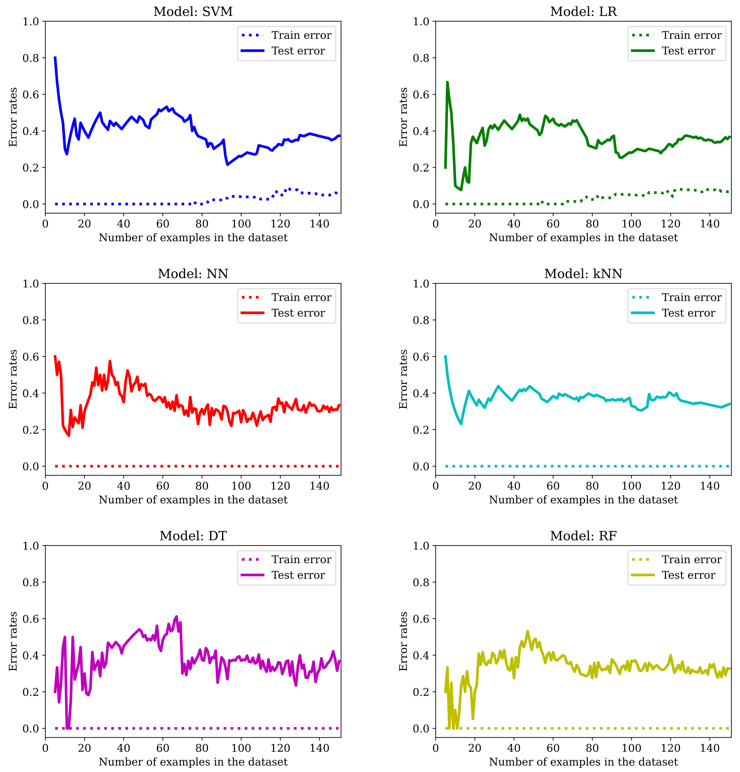
The main drawback of applying machine learning techniques to data acquired in studies involving patients (or humans in general) is the limited amount of available examples. It is well known that the more data we get, the better the outcome—at least once the complexity of the model used in the learning process is adjusted accordingly. In this particular study, we only have 77 subjects, and obtaining more data by amplifying the list of participants was not an option. As we can see from Figure 7, by training the six models mentioned in Section 2.5 with an increasing number of examples, we get too-high error rates for unseen data.

The error rates reported in Table 2, which will serve us as a baseline, were obtained by using mainly the default values of the meta-parameters of the models, with these small modifications:

• SVM was trained with the linear kernel and no regularization ($C=1$). Although the name of the kernel is misleading, making us think that there is a transformation of the original points from ${\mathbb{R}}^{126}$ to ${\mathbb{R}}^{77}$, this does not actually happen; technically speaking, we would get the same prediction using a linear kernel or an SVM without kernel, so the implementation of the SVM in sklearn avoids performing unnecessary calculations. Thus, the “linear kernel” in reality is “no kernel”.
• LG was trained without regularization ($C=1$).
• The number of neighbors in kNN was chosen to be 1.

In the first row of the table (indexed as LOO), the evaluation is performed using the Leave One Out cross-validation method. In the second one (indexed as Train/test), the error rates are computed for the randomly selected train and test set of 50 and 27 entries, respectively (more details can be found in Section 2.6). The models were built using the methods provided by the sklearn package [32].

Table 2. Error rates for the OrigD dataset (default values).

Error Rates	SVM		LR		NN		kNN		DT		RF
	Train	Test	Train	Test	Train	Test	Train	Test	Train	Test	Train	Test
LOO	0.000	0.273	0.000	0.312	0.000	0.260	0.000	0.325	0.000	0.416	0.000	0.325
Train/test	0.000	0.370	0.000	0.333	0.000	0.333	0.000	0.333	0.000	0.370	0.000	0.296

Table 2. Error rates for the OrigD dataset (default values).

Error Rates	SVM		LR		NN		kNN		DT		RF
	Train	Test	Train	Test	Train	Test	Train	Test	Train	Test	Train	Test
LOO	0.000	0.273	0.000	0.312	0.000	0.260	0.000	0.325	0.000	0.416	0.000	0.325
Train/test	0.000	0.370	0.000	0.333	0.000	0.333	0.000	0.333	0.000	0.370	0.000	0.296

For the sake of self-containment, we also provide the details of the architecture of the NN—we used the sklearn implementation of a Multi-layer Perceptron (MLP) classifier: one hidden layer with 100 neurons per layer with the Relu activation function.

We can see that the best models are NN and RF. However, the error rate in the training set is always zero and there is a big gap between the Train error and the Test error. Training with more examples usually helps: if the error in the test set is around 40% in most cases with 38 examples in the training set (see Figure 7), it goes down to roughly one-third of the data with 50 examples in the training set and to even lower values for most of the models listed in Table 2 when LOO cross-validation is used (in this case, 76 of the examples are used for training). This is a clear indication of overfitting. So, we will dedicate the following sections to show the effect of applying the typical mitigation techniques to our dataset: feature selection (Section 3.1), regularization (Section 3.2), increasing the dataset size (Section 3.3), meta-parameters fine-tuning (Section 3.4), or combining all of the above (Section 3.5).

3.1. Feature Selection

One way to avoid overfitting is by using only some of the predictors (also called features), normally those that are thought to be representative of the problem at hand. This selection can be made either manually (by an expert) or automatically (by means of algorithms). In this case, we opt for the first one, since we already have a list of predictors that were identified as relevant in distinguishing between a PD patient and a participant from the HC group in a previous study [22,33], as mentioned in Section 2.4. Whenever we refer to a dataset with selected features, we add a ${}^{*}$ to its name: OrigD${}^{*}$ will denote the original dataset from which we only keep 19 selected columns.

The evolution of the error rates with increasing number of examples is plotted in Figure 8. It is clear that while the SVM and the LR do benefit from feature selection, none of the other models manage to avoid having a null training error rate (at least not with this small number of examples).

However, as one can see in

Table 3. Error rates for the original data set with selected features (OrigD${}^{*}$).

Error Rates	SVM		LR		NN		kNN		DT		RF
	Train	Test	Train	Test	Train	Test	Train	Test	Train	Test	Train	Test
LOO	0.261	0.442	0.304	0.416	0.000	0.442	0.000	0.455	0.000	0.545	0.000	0.286
Train/test	0.220	0.333	0.240	0.296	0.000	0.407	0.000	0.481	0.000	0.296	0.000	0.296

, the error rates are notably bigger for the LOO evaluation metric (with only one exception: the RF model) and there is a slight improvement for the SVM (from 0.370 to 0.333), LR (from 0.333 to 0.296) and DT (from 0.370 to 0.296) when training and testing with the fixed randomly selected examples.

In conclusion, we do avoid overfitting for SVM and LR; we get worse results for NN and kNN in both settings and we get better results (or at least not worse) for SVM, LR, DT and RF for the designated test set (but the improvement is not significant).

3.2. Regularization

The term “regularization” in machine learning is a form of regression that constrains or shrinks the coefficient estimates towards zero. As such, it is not applicable to any model. The idea is to discourage learning a more flexible or complex model in order to avoid overfitting. In particular, three of the models employed in this study, namely the SVM, the LR and the NN, have a specific way of introducing regularization: adding the squared $L_1$ or $L_2$ norm of the vector of weights (with the exception of the intercept term) to the cost function. One can either multiply this quantity by a parameter (usually called either $\lambda$ or $\alpha$—the bigger its value, the more regularization is introduced) or multiply the other part of the cost function by a parameter C (smaller values correspond to more regularization).

For kNN, the only “regularization” proposal that we are aware of is to give different importance to the features depending on how relevant they are for the problem when computing distances between points. The greater the regularization parameter, the more it penalizes features that are not correlated with the target variable. (https://towardsdatascience.com/a-new-better-version-of-the-k-nearest-neighbors-algorithm-12af81391682, accessed on 15 August 2022). Nevertheless, the kNN model from sklearn does not have this option implemented, and we believe that this approach is not exactly similar in spirit to the traditional regularization, since it does not equally penalize all weights. Therefore, we will not apply regularization techniques in this case. As for the DT and RF models, the only way to introduce regularization in the sklearn implementation is via the maximum depth of the trees. However, it is arguable if this approach can really fit under the regularization umbrella and, on the other hand, we will explore this possibility in Section 3.4 as one way of fine-tuning the meta-parameters of the model.

Note that finding the best value for the regularization parameter can be achieved by trying with different values (for example, 0.0001, 0.001, 0.01, 0.1) and picking the one that performs best—but not for the test set, because we want the Test error rate to be obtained with data that have not be seen by the algorithm at all. That is why we chose the regularization parameter value by performing 10-fold cross-validation on the training set. The value obtained for SVC was C = 0.01 (with the $L_2$ norm), for LR was C = 0.1 (with the $L_1$ norm and the liblinear solver), and for NN was alpha = 10 (with the $L_2$ norm).

The results obtained are presented in Figure 9 and

Table 4. Error rates for the original data set when using regularization.

Error Rates	SVM		LR		NN		kNN		DT		RF
	Train	Test	Train	Test	Train	Test	Train	Test	Train	Test	Train	Test
LOO	0.135	0.273	0.190	0.234	0.021	0.286	-	-	-	-	-	-
Train/test	0.080	0.296	0.200	0.185	0.020	0.296	-	-	-	-	-	-

. We conclude that regularization does help avoid overfitting in all cases, to the point that LR performs worse in training than in the test set in the beginning. It is noteworthy that the accuracy of the LR model in the test set is 81.5%, a very promising value.

3.3. Increasing the Size of the Dataset

One way of obtaining more data is to calculate the values of the predictors for each segment walked instead of using the average over all segments. Note that the number of segments covered is variable: in the first experiment, participants walked between one and six valid segments, in the second experiment only one (since the task was precisely to walk the whole length of the corridor as fast as possible) and in the third experiment, between two and five. The three values represented in each cell of

Table 5. Minimum, maximum and average number of segments (per group and overall).

	Min	Max	Average
PD group	1/1/2	5/1/5	3.73/1/3.61
HC group	3/1/2	6/1/5	4.31/1/4.36
All participants	1/1/2	6/1/5	4/1/3.82

correspond to the three experiments: experiment 1/experiment 2/experiment 3.

Since we cannot have a variable number of predictors, one idea is to generate multiple entries for each participant by combining, in all possible ways, all the segments of the first experiment with the only segment in the second experiment, and with all the segments of the third experiment. Thus, if we denote by $n_i$ the number of segments in experiment i (with i in $\{1,2,3\}$) for a given participant, then the total number of entries associated with this participant in the new dataset will be $n_1\times n_3$ (recall that $n_2$ is always one). We will refer to this dataset as BigD—it has 1202 rows and the same number of columns as the original one (126).

An additional precaution now is to always make sure that entries of the same participant are never present in both the training and test set (otherwise accuracy values might be artificially inflated, since some examples under evaluation in testing would share exactly the same values for at least 42 out of the 126 predictors). This is achieved by working with batches of examples. For instance, when calculating the error rates within the LOO evaluation framework, “the” one example being tested in the current iteration is actually composed of all entries corresponding to a given participant (and the average value is reported). A similar strategy is used to build the new training and testing set. A slightly different approach is used for the error rates in the case of the train/test sets of increasing size, since participants do not have a fixed number of rows. In this case, we first build the new train/test sets and then we use the first n entries to train or test the models (with n in $\{17,\dots ,587\}$).

The evolution of error rates with an increasing number of examples shows no improvement (see Figure 10). One major difference that can be perceived in the initial stages of training the DT model is that the test error rate stabilizes around the 40% value only after seeing half of the total number of examples.

As we can see from the previous graphs and from the error rates, artificially creating more data this way does not help avoid overfitting in any of the six models. Additionally, with a few exceptions, the results are generally worse (

Table 6. Error rates for the BigD data set (default values).

Error Rates	SVM		LR		NN		kNN		DT		RF
	Train	Test	Train	Test	Train	Test	Train	Test	Train	Test	Train	Test
LOO	0.001	0.383	0.004	0.336	0.000	0.345	0.000	0.364	0.000	0.310	0.000	0.322
Train/test	0.000	0.440	0.000	0.328	0.000	0.287	0.000	0.409	0.000	0.338	0.000	0.307

).

We believe that one of the main drawbacks is that many of the entries have blocks of identical values, so, instead of avoiding the overfitting, we create more of it. Clearly, obtaining more data this way is not helping because, although we can see some improvements in some numbers, the zero error rate in training is not a good sign. In Section 3.5 we see how it works combined with feature selection/regularization/fine-tuning.

Another idea for obtaining more data is to keep only the predictor values from one of the three experiments (the number of features goes down from 126 to 42), creating one entry per segment walked. This way, we avoid having shared information within two different entries. We chose experiment 1, but the same analysis can be extended to the other two experiments (of course, if we select the second experiment then there is no data augmentation: we would have the same number of rows with fewer columns). Note that the number of examples in the graphs of Figure 11 go from 5 (this allows us to have at least one positive and one negative entry) to 150.

By checking the error rates from

Table 7. Error rates for the MedD data set (default values).

Error Rates	SVM		LR		NN		kNN		DT		RF
	Train	Test	Train	Test	Train	Test	Train	Test	Train	Test	Train	Test
LOO	0.142	0.355	0.160	0.359	0.000	0.283	0.000	0.388	0.000	0.316	0.000	0.310
Train/test	0.065	0.383	0.075	0.336	0.065	0.262	0.000	0.393	0.000	0.364	0.000	0.280

, we can see that the Train error is not zero anymore for SVM, LR and NN, and that both models that involve trees (DT and RF) have improved their score. Additionally, four of the six models in Figure 11 show a clear overfitting pattern. Recall that these results are obtained without fine-tuning the meta-parameters (this will be carried out in Section 3.5).

3.4. Fine-Tuning Meta-Parameters

In this section, we describe all the meta-parameters that have been fine-tuned for each model. The methodology followed was the same in all cases: a range of values was provided for each parameter and the GridSearch method would fit 10 different models for each possible combination (via 10-fold cross validation, with 90% of data for training and the other 10% for testing). The score for one particular combination of meta-parameters (with their corresponding values) is calculated as the mean of the accuracy rate over the 10 folds. In the end, the best combination is saved to disk, along with the Train error (this time computed over the whole training set) and test error, as usual. Note that this approach does not necessarily produce the model with the best accuracy in the test set, but it has the advantage of providing a fair estimate of how the model would behave with unseen data. It should also be noted that some of the models we train are not deterministic, which means that different runs of the algorithm would report distinct values (in particular, NN are stochastic models and the choice of features in RF is random).

In the case of SVM, we have varied the regularization parameter C: nine values in the range [0.0001, 1] and the kernel: linear, polynomial (poly), Gaussian (rbf) and sigmoid. For the polynomial kernel, we have tried using polynomials of degree 2, 3 and 4 and the kernel coefficient gamma oscillated between scale (the value of gamma is one divided by the product between the number of features and the variance of the training set) and auto (the value of gamma is one divided by the number of features) for all but the linear kernel (which does not have a kernel coefficient).

The meta-parameters fine-tuned for LR were: C, the regularization parameter (thirteen values in the range [0.0001, 10]), and the solver (liblinear and saga with $L_1$ and $L_2$ penalties, and lbfgs, newton-cg, sag with either the $L_2$ penalty or no penalty).

Many more meta-parameters were considered in the case of NN: the architecture of the network (one hidden layer with 10, 50 or 100 neurons), the activation function (tanh, relu or sigmoid), the solver (sgd or adam), the learning rate (constant or adaptive), the maximum number of iterations (20, 50, 100 or 200), the regularization parameter alpha (ten values in the range [0.0001, 100]), the momentum for gradient descent update (0.6, 0.9 or 0.95, used only for the sgd solver) and early_stopping: True or False (From sklearn documentation: “Whether to use early stopping to terminate training when validation score is not improving. If set to true, it will automatically set aside 10% of training data as validation and terminate training when validation score is not improving by at least tol for n_iter_no_change consecutive epochs”).

The number of neighbors considered for NN was 1, 3, 5, 7 or 9. The weights parameter was either uniform (the weights of all points in a neighborhood are the same) or distance (the weight of each point is the inverse of their distance), the algorithms used were ball_tree or kd_tree or brute (uses a brute-force search), the leaf_size (only valid for ball_tree and kd_tree, can affect the speed and the memory used) was set to 10, 30 or 50 and p was one (Manhattan distance a.k.a. $L_1$), 2 (Euclidian distance = $L_2$ norm) or three (Minkowski distance, $L_3$).

For DT, three different criteria were explored for branch ramification: gini, entropy and log_loss. The splitter (the strategy used to choose the split at each node) was either best or random. The max_depth was None, one, three or five, the min_samples_split (that is, the minimum number of samples that are necessary in order to split an internal node) was always two, and max_features was None (all features are considered), sqrt (the square root of the number of features) or log2 (logarithm in base two of the number of features).

In the case of RF, the max_depth, min_samples_split and max_features had the same range of values as for DT. In this case, we explored only two branch ramification criteria: gini and entropy, and the number of estimators was 10, 50 or 100 (whenever possible).

Since the fine-tuning of the meta-parameters was carried out for all datasets when searching for the best model, we postpone reporting on the results obtained with the original dataset (OrigD) to the next section.

3.5. Finding the Best Model

So far, we have explored applying different techniques to one particular dataset, but, when doing so, we have created new datasets (with more rows or less columns). In this section, we show the results obtained when applying the methodology described in Section 3.4 to each of the six datasets we have been working with: OrigD (77 rows, 126 columns) and its smaller version OrigD${}^{*}$ (77 rows, 19 columns) obtained via feature selection, BigD (1202 rows, 126 columns) and BigD${}^{*}$ (1202 rows, 19 columns), MedD (308 rows, 42 columns) and MedD${}^{*}$ (308 rows, 5 columns).

To be succinct, we omit graphics and we include only the error rates (see

Table 8. Error rates for all datasets when fine-tuning meta-parameters.

Error Rates	SVM		LR		NN		kNN		DT		RF
	Train	Test	Train	Test	Train	Test	Train	Test	Train	Test	Train	Test
OrigD	0.080	0.296	0.200	0.185	0.000	0.259	0.000	0.296	0.000	0.296	0.040	0.259
OrigD${}^{*}$	0.160	0.259	0.320	0.259	0.360	0.222	0.280	0.259	0.000	0.333	0.260	0.259
BigD	0.077	0.275	0.028	0.299	0.047	0.236	0.000	0.365	0.182	0.202	0.182	0.202
BigD${}^{*}$	0.314	0.299	0.315	0.229	0.327	0.204	0.000	0.421	0.322	0.438	0.174	0.229
MedD	0.070	0.318	0.164	0.290	0.224	0.290	0.000	0.393	0.318	0.290	0.000	0.243
MedD${}^{*}$	0.289	0.280	0.299	0.271	0.308	0.243	0.000	0.271	0.348	0.280	0.269	0.243

). As mentioned before, we always search for the best parameters for the dataset under study with 10-fold cross-validation on the training set, and thus the chosen model might not be the best for the test set. Fine-tuning meta-parameters includes regularization for the SVM, LR and NN models.

We can see that for each dataset there is at least one model that has an accuracy rate for unseen data of at least 74%, that none of the models is the best for all datasets (something to be expected—see the No Free Lunch Theorem [34]) and that the smallest error rates are around the 20% mark.

We have emphasized in boldface the best value of each column in the test set and in blue, the best model for each dataset. In

Table 9. Best values of the meta-parameters for each model.

Model	Dataset	Parameters and Values
SVM	OrigD${}^{*}$	kernel = poly, probability = True
LR	OrigD	C = $0.1$, penalty = l1, solver = liblinear
NN	BigD${}^{*}$	alpha = 33, early_stopping = True,
		hidden_layer_sizes = $(50,)$, learning_rate = adaptive
kNN	OrigD${}^{*}$	algorithm = ball_tree, leaf_size = 10,
		n_neighbors = 7, p = 3
DT	BigD	max_depth = 1
RF	BigD	max_depth = 1, max_features = None

we give, for each model, the values of the meta-parameters that had the best outcome, along with the corresponding dataset (every parameter whose value is not set is understood to have a default value):

4. Discussion

The first thing to notice from analyzing the results in Table 8 is that most of the models’ best versions are not prone to overfitting. The most notable exception is the kNN: in five out of six cases, the error rate in training is zero, so we would not recommend applying this method for diagnosing PD patients. On the other hand, the rest of the models seem to have overcome this issue in all or almost all of the datasets under study.

For the best model (Logistic Regression for the OrigD dataset), we present the rest of the indicators detailed in Section 2.6. The accuracy is 81.5%, AUC 0.879, sensitivity 0.71, specificity 0.92 and precision 0.91. The 95-confidence interval is 0.147, and the confusion matrix and the ROC curve are presented in

Table 10. Confusion matrix for the test set of OrigD and the best LR model.

Real/Predicted	PD	HC
PD	10	4
HC	1	12

and Figure 12, respectively.

Note that the model has very high specificity and precision and lower recall. This means that there will be more PD patients that the model will not be able to identify as such (four in this test set). Ideally, we should pick a model that minimizes this quantity, but none of the other models listed in Table 9 is better in this respect.

An accuracy above 80% for a system that learns only from gait statistics (mean and standard deviation values of measurements such as the step length or the arm amplitude), which can be automatically obtained from people walking a corridor while wearing a set of 16 sensors, is quite impressive, given the small amount of available data. We believe that we have practically exhausted all possibilities in this study, and little can be done to further improve this number. In future work, we would like to explore more complex models that use the raw data obtained from the sensors instead of the gait statistics—there might be information that we are not yet aware of, which differentiates PD patients from the rest.

5. Conclusions

In previous studies, we have analyzed to what extent alternations of gait parameters are correlated with the PD diagnosis. Thus, we could see that PD patients showed differences in arm swing and stride length asymmetry, variability and amplitude, and also in speed. Moreover, some differences were perceived in step and stride time. Here, we employ machine learning tools to learn models that are able (up to a certain point) to distinguish between PD patients and controls by using some or all of the gait parameters extracted in the preprocessing phase. Although the sensor-based detection system that we built is far from being perfect, we believe that it is a promising research venue and that, in the future, we can hope for more robust models (trained with more data) that will be able to place a diagnosis in the early stages of the disease by simply interpreting the data provided by the inertial sensor system.