Article

Scalar Variance and Scalar Correlation for Functional Data

by
Cristhian Leonardo Urbano-Leon
1,*,†,
Manuel Escabias
1,†,
Diana Paola Ovalle-Muñoz
1,† and
Javier Olaya-Ochoa
2,†
1
Department of Statistics and Operations Research, University of Granada, 18071 Granada, Spain
2
School of Statistics, University of Valle, Cali 760042, Colombia
*
Author to whom correspondence should be addressed.
These authors contributed equally to this work.
Mathematics 2023, 11(6), 1317; https://doi.org/10.3390/math11061317
Submission received: 3 February 2023 / Revised: 2 March 2023 / Accepted: 4 March 2023 / Published: 9 March 2023

Abstract

:
In Functional Data Analysis (FDA), the existing summary statistics so far are elements in the Hilbert space L 2 of square-integrable functions. These elements do not constitute an ordered set; therefore, they are not sufficient to solve problems related to comparability such as obtaining a correlation measurement or comparing the variability between two sets of curves, determining the efficiency and consistency of a functional estimator, among other things. Consequently, we present an approach of coherent redefinition of some common summary statistics such as sample variance, sample covariance and correlation in Functional Data Analysis (FDA). Regarding variance, covariance and correlation between functional data, our summary statistics lead to numbers instead of functions which is helpful for solving the aforementioned problems. Furthermore, we briefly discuss the functional forms coherence of some statistics already present in the FDA. We formally enumerate and demonstrate some properties of our functional summary statistics. Then, a simulation study is presented briefly, with evidence of the consistency of the proposed variance. Finally, we present the implementation of our statistics through two application examples.

1. Introduction

Functional Data Analysis (FDA) is a branch of statistics that has played a growing role since the book by [1] due to its multiple applications [2,3,4,5,6,7,8]. In fact, according to [9], the term Functional Data Analysis is due to [10,11], although some previous work on the subject is credited to [12,13]. FDA takes, as a starting point, discrete measurements of a continuous phenomenon to construct smooth curves using modified numerical analysis techniques. With these, the set of scalar data is converted into a new object called a functional datum, which is a continuous function [8,14]. This allows us to bring into statistical analysis some theoretical aspects from functional analysis, where some sets of functions with certain characteristics can form algebraic structures [15,16]. These structures can provide optimal properties for the analysis and measurement of continuous function curves. The Hilbert space, which is formed by square-integrable functions in a closed interval [ a , b ] ; a , b R , is a structure that plays a key role in this context. It is usually denoted as L 2 [ a , b ] and the main reason for playing such an important role is because Hilbert spaces are usually seen as extensions of the Euclidean space [15,17] (pages 249 and 19, respectively) because they have distance and size measures [18], which are desirable properties.
Until now, most existing FDA theory has been constructed based on the extension of scalar statistics concepts to functions, giving functional objects as a result. For instance, a widely accepted definition of summary statistics for functional data is given in [1], who define the sample functional mean, variance, covariance and correlation as continuous functions in L 2 [ a , b ] , as shown in Definition 1.
Definition 1.
Measures in Functional Data: Given the sets of functional data X i i = 1 n and Y i i = 1 n defined in t a , b , the summary functions are defined as:
  • Mean:
    X ¯ ( t ) = i = 1 n X i ( t ) n
  • Variance:
    V a r ( X ) ( t ) = i = 1 n ( X i ( t ) X ¯ ( t ) ) 2 ( n 1 )
  • Standard Deviation:
    S d ( X ) ( t ) = V a r ( X ( t ) )
  • Covariance:
    C o v ( X , Y ) ( t ) = i = 1 n ( X i ( t ) X ¯ ( t ) ) ( Y i ( t ) Y ¯ ( t ) ) ( n 1 )
  • Correlation:
    C o r r ( X i , Y i ) ( t ) = C o v ( X , Y ) ( t ) S d ( X ) ( t ) S d ( Y ) ( t )
In Definition 1, we show an expression for the covariance between X and Y , which is usually defined in the literature as “cross-covariance”. This name is suggested by Ramsay and Silverman in their 2005 book because they define the covariance as a summary of the dependence of records across different argument values.
It should be noted, however, that functions and scalars are different mathematical objects with different properties, which generates some conceptual discussions. Let us consider in the first place the functional mean. As is very well known for scalar data [19] (pp. 15–18), the Arithmetic Mean is a central tendency indicator that must be interpretable in the same context as the data. In this sense, the fact that the functional mean is a function results in a conceptually coherent concept of “tendency” because the functional mean describes the expected behavior of a set of functions related to a functional random variable. Moreover, it also has the property of “centrality” [20] (p. 76), which can be described in its functional form with the fulfilment of Equation (1), where X 0 is the null function in the definition interval of the functional dataset { X i } ( i = 1 ) n .
i = 1 n ( X i X ¯ ) = X 0
However, if we follow the approach of [1], proving this fact requires an exhaustive walkthrough of the infinite points of the function’s definition interval, which adds complexity to a proof that would become simpler upon performing the new approach we propose in this paper.
Let us consider now the functional variance. It should be considered that the usual motivation for the concept of variance is as a measure of dispersion [21] (p. 309), whose initial intention is to bring a comparative way for the use of consistency and efficiency concepts [22,23], whose definition is based on the basic premise that the sum of the squares of the deviations from the mean is a minimum [19] (pp. 555–557). Namely, given a set of scalar data { x i } i = 1 n , n N , associated with the random variable X and whose arithmetic mean is X ¯ , the sum of Expression (2) is minimum value when a = X ¯ [20] (p. 84), so that the variance in Expression (3) is also minimum value because it reflects the expected behavior of the deviations from the mean.
i = 1 n ( x i a ) 2
1 n i = 1 n ( x i X ¯ ) 2
Similarly, given a functional dataset X i i = 1 n and a functional datum Y , the sum in Expression (4) must be minimum value when Y = X ¯ , where X ¯ is the functional mean of X i i = 1 n .
i = 1 n ( X i Y ) 2
However, Ramsay and Silverman’s functional variance given in Definition 1 does not comply with this functional version of such property. This is true because the concept of a “minimum” function lacks validity due to the functional character of the objects and that the functions do not form a well ordered set [24,25,26].
Furthermore, a conceptual problem seems to be associated with the fact that the variance itself gives a measure of the distance from the values to the mean [21]. According to [17], a measure always has to be a nonnegative real number; therefore, the functional variance given in Definition 1 is not truly a measure of dispersion of the functional data but rather a curve that offers point-to-point variances within the functional data definition interval.
Another important flaw of the variance curve is that, due to the lack of order inside a functional space, if there are two sets of curves, it is hard to decide which of the two sets has a larger dispersion. This is possible, however, with a point-to-point comparison, as is done if we look at the functional variance as a curve of point-to-point variances.
On the other hand, on the functional covariance and correlation, while the concept of covariance is not thought of as a measure, it is expected to be an indicator of the joint variation of two random variables [27,28]. It maintains a close relation to the concept of variance because the variance is a very particular case of the covariance [19] (pp. 126–128). Therefore, if the functional variance is a real number, the covariance must also be because there should be coherence between the concepts. However, covariance in Definition 1 is just a point-to-point covariance function whose interpretation gives an idea of the regions where there is a larger or a smaller joint variation of the curves within the definition interval of the functional data, but it is not an indicator of the joint variation of two functional random variables.
In turn, correlation is defined as a coefficient that is linked to the concept of covariance [19] (pp. 115–119) and for that reason, it must be defined as a real number, even in functional data. However, it is important to point out that the concept of “linear” correlation within functional data does not become clearly visible and its “linear” interpretation needs further study.
In this sense, we present a new approach for the treatment of functional data that attempts to provide summary statistics for functional data with conceptual coherence and operational advantages, defining the variance, covariance and correlation for functional data as real numbers. For this, we use one of the most notable particularities of the Hilbert spaces like vector space because, as claimed by [29,30,31,32], the elements of a vector space can be uniquely completely described by a linear combination of a set of orthogonal elements called a basis. However, for L 2 [ a , b ] , this set is infinite. For that reason, all FDA theory is not performed over the entire L 2 [ a , b ] but over a subspace of finite dimension [33] because the number of functions used as a basis for the construction of the functional data is finite [1,34].
Thus far, this fact has been little explored in FDA theoretical development, although there are recent works, such as [35], that estimate a test statistic using the basis coefficients, the use of coefficients in the homogeneity problem by [36], and also [37] who use the basis coefficients for estimating functional PLS regression, or even previously, with the use of principal components of functional logistic regression the authors of [38] deal with some aspects of the subject. However, our approach addresses the functional data from a vector perspective because each functional datum corresponds to a single coefficient vector that characterizes it, which allows transferring some operations between functions to operations between coefficient vectors, component-by-component, providing operational advantages in formal proofs.
It is important to point out that our approach is based on the representation of a continuous function within an arbitrary subspace of finite dimension of L 2 [ a , b ] 
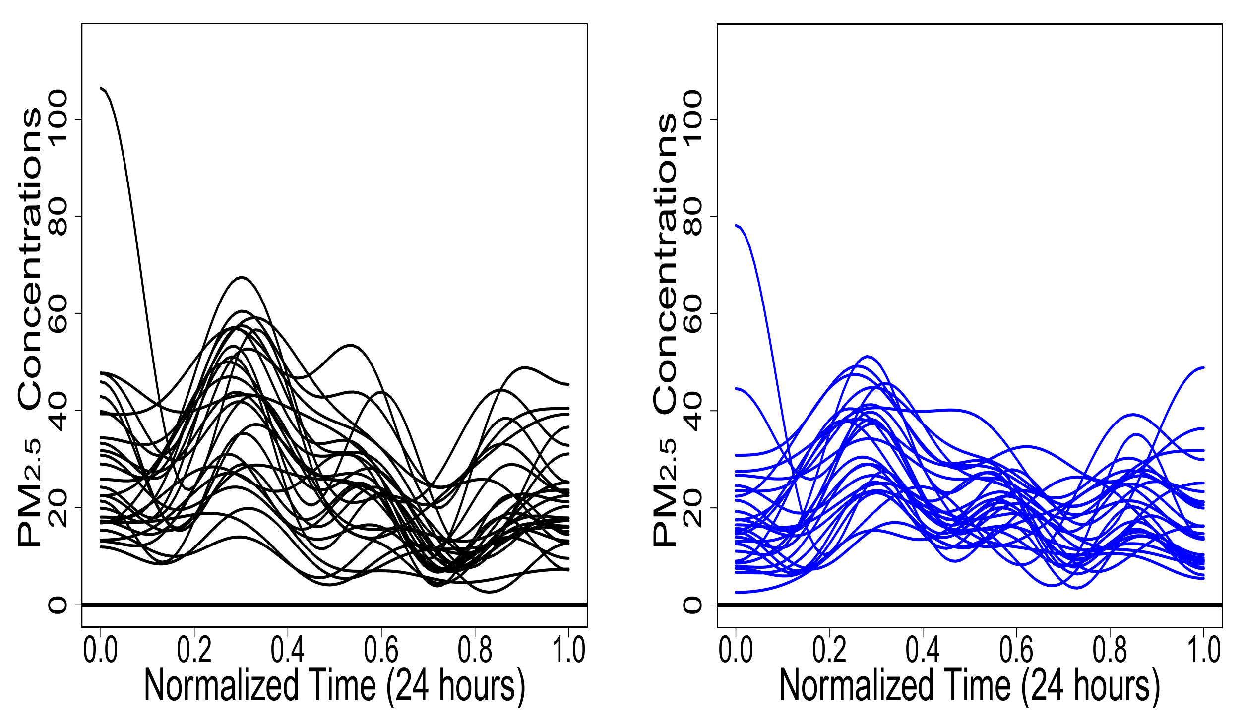
and therefore the results obtained can be applied without loss of generality to any type of orthonormal basis and of any finite dimension. Thus, in addition to the theory proposed, a simulation study with curves represented in a subspace spanned by an orthonormal basis of cosines in the [0, 1] interval is presented briefly and two implementation examples are described in the final section. In the first example, we implement our correlation proposition to determine whether there is independence between the functional random variables, used by [1] when constructing a functional analysis of variance (FANOVA) of the Canadian average annual temperature in four of its regions. This is done because the analysis does not specify the existence of independence between the functional random variables. The second example describes the use of our variance and functional correlation proposition as part of a functional and descriptive data analysis on particulate matter from two air quality monitoring stations in Cali, Colombia.
At this point, we recall some very well known background information, which we will need to present the new summary statistics definitions.
Definition 2.
System of Generators, Basis and Dimension:
  • Given a vector space V over a field K and given S V , it is decided that V is spanned by S if every element of V can be written as a linear combination of the elements of S [32].
  • A vector space is said to be of finite dimension if it can be generated by a finite set of elements [39].
  • A set B V is a basis for V if B spans V and is also linearly independent [32].
Definition 3.
Hilbert Space: In a very general manner, a Hilbert space is a vector space over the field of real numbers in which a norm and an inner product have been defined [34,40].
Definition 4.
Functional Space: A functional space is a vector space whose elements are functions.
Definition 5.
The Functional Hilbert Space L 2 [ a , b ] : The L 2 [ a , b ] space is a vector space over the field of real numbers whose elements are square-integrable functions in the closed interval [ a , b ] ; a , b R and where given f , g L 2 [ a , b ] , an inner product, a norm and a distance are defined as:
  • Inner product: f , g = a b f ( x ) g ( x ) d x .
  • Norm: f = f , f 1 / 2 = ( a b f 2 ( x ) d x ) 1 / 2
  • Distance: d f , g = a b f ( x ) g ( x ) 2 d x
With this, the L 2 [ a , b ] space is a functional Hilbert space [29,41].
Definition 6.
Orthonormal and Orthogonal Bases: Two elements of a vector space are orthogonal if and only if the inner product between them is zero. In the same way, an element of a vector space is said to be normal if and only if its norm value is equal to 1. Thus, a basis is said to be orthogonal if and only if it is composed of elements that are orthogonal two-by-two. If, in addition, such elements satisfy the condition of normality, the basis is said to be orthonormal [30,42].
Definition 7.
Functional Random Variable: A functional random variable X is a random variable that takes values in a functional space, where an observation of X is called a functional datum [43].

2. Summary Statistics for Functional Data

With the motivation of providing FDA theory with summary statistics that have interpretive and operational advantages, in this section, we propose a new approach for the treatment of functional data that considers them as elements of the same functional subspace H of finite dimension of the Hilbert space L 2 [ a , b ] , which allows transforming operations between functions to operations between elements of vectors of coefficients component-by-component because the L 2 [ a , b ] space is in particular a vector space and therefore if B = F j j = 1 p is a finite basis of H and X H , defined on Equation (5), is a functional datum,
X = j = 1 p a j F j For a j R with j = 1 , 2 , 3 , , p .
where X is a linear combination of the elements of B and therefore X is uniquely completely determined by the vector a 1 , a 2 , a 3 , , a p B , which is called the B basis representation vector.
As mentioned, Ref. [35] estimate a test statistic using the basis coefficients. Previously, on a density estimation problem, Ref. [33] used a finite-dimensional approximation of the functional data, just like the one we propose here. However, none of them moved toward the representation of summary statistics for functional data using the vectors of coefficients used for the functional data representation shown in Equation (5). Next, the new definitions of summary statistics are proposed, as well as their properties.

2.1. Sum of Functional Data

As observed in works by [44,45] and in most of the textbooks on linear algebra and functional analysis, the sum of the elements of a space of finite dimension can be defined by the sum of their representation coefficients in the same basis, as is presented in Proposition 1 and whose proof is immediate, using the representation of each functional datum and the association and commutation properties of L 2 [ a , b ] under the sum.
Proposition 1.
Let H be a subspace of finite dimension p of the Hilbert space L 2 [ a , b ] with basis B = F j j = 1 p and X i i = 1 n H a set of n functional data with representation vectors a i , 1 , a i , 2 , , a i , p B , for some a i , j R with i = 1 , 2 , n and j = 1 , 2 , 3 , , p . Then, the sum i = 1 n X i is an element of H with representation vector:
i = 1 n a i , 1 , i = 1 n a i , 2 , , i = 1 n a i , p B
Proof. 
Given that a i , 1 , a i , 2 , , a i , p B with a i , j R , i = 1 , 2 , n and j = 1 , 2 , 3 , , p are representation vectors,
i = 1 n X i = i = 1 n j = 1 p a i , j F j = j = 1 p i = 1 n a i , j F j
Therefore, given F j H for every 1 j p , then i = 1 n X i H and its representation vector is
i = 1 n a i , 1 , i = 1 n a i , 2 , , i = 1 n a i , p B
Proposition 1 indicates that the sum of the n functional data X i i = 1 n is completely determined by the sum of the representation vectors component-by-component.

2.2. Mean of Functional Data

It is possible to obtain a definition of the mean for functional data from the representation coefficients, as we show in Proposition 2 and whose proof applies Proposition 1 as well as the representation coefficients.
Proposition 2.
Let H be a subspace of finite dimension p of the Hilbert space L 2 [ a , b ] with basis B = F j j = 1 p and X i i = 1 n H a set of n functional data with representation vectors a i , 1 , a i , 2 , , a i , p B for a i , j R with i = 1 , 2 , , n and j = 1 , 2 , , p . Then, the functional mean for the functional dataset X i i = 1 n is given by:
X ¯ = j = 1 p A ¯ j F j
where A ¯ j = 1 n i = 1 n a i , j for j = 1 , 2 , , p
Proof. 
Given A ¯ j = n 1 i = 1 n a i , j is the mean of the j t h coefficients with j = 1 , 2 , , p , then:
X ¯ = 1 n i = 1 n X i = 1 n i = 1 n j = 1 p a i , j F j = j = 1 p 1 n i = 1 n a i , j F j = j = 1 p A ¯ j F j
Proposition 2 indicates that the representation vector of the functional mean is completely determined by the representation vector of component-by-component mean coefficients. Namely, for a set of n functional data whose representation vectors are a i , 1 , a i , 2 , , a i , p B with 1 i n , the functional mean is another functional datum, whose representation vector is A ¯ 1 , A ¯ 2 , , A ¯ p B .
In addition, it should be noted that the functional mean of Proposition 2 and the one in Definition 1 are the same functions because, as mentioned above, it is coherent with the concept of tendency. However, under this new approach, the functional mean has operational advantages, some of which are immediately observed in the proof of the functional version of the property of centrality (p. 76, [20]), illustrated by Proposition 3.
Proposition 3.
Let H be a subspace of finite dimension p of the Hilbert space L 2 [ a , b ] , X i i = 1 n H a set of n functional data and X ¯ its functional mean, then:
i = 1 n ( X i X ¯ ) = X 0
where X 0 is the null function in [ a , b ] .
Proof. 
Let B = { F i } i = 1 p be a basis of H . Therefore, there are a i , j R such that X i = j = 1 p a i , j F j for every i = 1 , 2 , n . In addition, by Proposition 2, X ¯ = j = 1 p A j ¯ F j , where A j ¯ = 1 n i = 1 n a i , j ; then, by Proposition 1:
i = 1 n X i X ¯ = i = 1 n j = 1 p a i , j A j ¯ F j = j = 1 p i = 1 n a i , j A j ¯ F j = j = 1 p 0 F j = X 0
because i = 1 n a i , j A j ¯ = 0 for j = 1 , 2 , , p , “ a i , j ” and “ A ¯ j ” are scalars and therefore satisfy the property of centrality. □

2.3. Variance for Functional Data

We define the variance for functional data as the average of the squared distances of each function to the functional mean. The distance used is the distance between the functions of L 2 [ a , b ] , shown above in Definition 5, which gives a scalar number as a result and therefore the variance of Definition 8 is a scalar and maintains the concept of the variance as a measure of dispersion because it is the expected behavior of the distances of the functions to the functional mean, whose interpretation is performed in a general manner over the entire set of functions.
Definition 8.
Variance for Functional Data: Let H be a subspace of finite dimension p of the Hilbert space L 2 [ a , b ] and let X i i = 1 n H be a set of n functional data associated with the functional random variable X ; then, the scalar variance for this functional data set is defined as:
V a r ( X ) = 1 n i = 1 n a b X i X ¯ 2 ( t ) d t
This definition allows having a scalar measure of dispersion, around the functional mean, of a set of functions. The most notable operational advantage of Definition 8 is given by Theorem 1.
Theorem 1.
Let H be a subspace of finite dimension p of the Hilbert space L 2 [ a , b ] , B = { F j } j = 1 p an orthonormal basis of H and X i i = 1 n H a set of n functional data associated with the functional random variable X , with representation vectors a i , 1 , a i , 2 , , a i , p B : 1 i n , then:
V a r ( X ) = j = 1 p V j
where V j = 1 n i = 1 n ( a i , j A j ¯ ) 2 .
Theorem 1 indicates that if the representation basis is orthonormal, the variance for the functional data can be simply calculated as the sum of the variances of the coefficients, component-by-component.
To prove Theorem 1, we need first to prove a couple of very important results presented in Lemmas 1 and 2.
Lemma 1.
Let H be a subspace of finite dimension p of L 2 [ a , b ] , B = { F j } j = 1 p a basis of H , { X i } i = 1 n H a set of functional data with representation vectors a i , 1 , a i , 2 , , a i , p B : 1 i n and Y H a functional datum with representation vector b 1 , b 2 , , b p B , then:
1 n i = 1 n X i Y 2 = j = 1 p 1 n i = 1 n ( a i , j b j ) 2 F j 2 + 2 k = 1 p 1 j = k p 1 1 n i = 1 n ( a i , j b j ) ( a i , ( j + 1 ) b ( j + 1 ) ) F j F ( j + 1 )
The proof of Lemma 1 follows from the representation of each of the elements of H on the selected basis and from the properties of summation.
Proof. 
Given that Y X i H for every i = 1 , 2 , , n , then:
1 n i = 1 n X i Y 2 =
= 1 n i = 1 n j = 1 p a i , j F j j = 1 p b j F j 2 = 1 n i = 1 n j = 1 p ( a i , j F j b j F j ) 2 = 1 n i = 1 n j = 1 p ( a i , j b j ) F j 2
= 1 n i = 1 n j = 1 p ( a i , j b j ) 2 F j 2 + 1 n i = 1 n 2 k = 1 p 1 j = k p 1 ( a i , j b j ) ( a i , ( j + 1 ) b ( j + 1 ) ) F j F ( j + 1 ) = j = 1 p 1 n i = 1 n ( a i , j b j ) 2 F j 2 + 2 k = 1 p 1 j = k p 1 1 n i = 1 n ( a i , j b j ) ( a i , ( j + 1 ) b ( j + 1 ) ) F j F ( j + 1 )
If in Lemma 1 we replace Y by the functional mean of { X i } i = 1 n , the Lemma 2 is obtained.
Lemma 2.
Let H be a subspace of finite dimension p of L 2 [ a , b ] , B = { F j } j = 1 p a basis of H , { X i } i = 1 n H a set of functional data with representation vectors a i , 1 , a i , 2 , , a i , p B : 1 i n and X ¯ the functional mean of { X i } i = 1 n ; then, if A j ¯ = 1 n i = 1 n a i . j , for 1 j p , the mean difference of squares can be decomposed as:
1 n i = 1 n X i X ¯ 2 = j = 1 p V j F j + 2 k = 1 p 1 j = k p 1 S a j , a j + 1 F j F j + 1
where V j = 1 n i = 1 n ( a i , j A j ¯ ) 2 and S a j , a j + 1 = 1 n i = 1 n ( a i , j A j ¯ ) ( a i , j + 1 A ¯ j + 1 ) .
Proof. 
By Lemma 1:
1 n i = 1 n X i X ¯ 2 = j = 1 p 1 n i = 1 n ( a i , j A j ¯ ) 2 F j 2 + 2 k = 1 p 1 j = k p 1 1 n i = 1 n ( a i , j A j ¯ ) ( a i , ( j + 1 ) A ¯ ( j + 1 ) ) F j F ( j + 1 )
but V j = 1 n i = 1 n ( a i , j A j ¯ ) 2 and S a j , a j + 1 = 1 n i = 1 n ( a i , j A j ¯ ) ( a i , j + 1 A ¯ j + 1 ) , with which:
1 n i = 1 n X i X ¯ 2 = j = 1 p V j F j 2 + 2 k = 1 p 1 j = k p 1 S a j , a j + 1 F j F j + 1
We thus provide a proof of Theorem 1.
Proof. 
By Definition 8:
V a r ( X ) = 1 n i = 1 n a b X i X ¯ 2 ( t ) d t
and by the integral’s properties, we know that:
1 n i = 1 n a b X i X ¯ 2 ( t ) d t = a b 1 n i = 1 n X i X ¯ 2 ( t ) d t
but from Lemma 2, we have that:
a b 1 n i = 1 n X i X ¯ 2 ( t ) d t =
= a b j = 1 p V j F j 2 ( t ) + 2 k = 1 p 1 j = k p 1 S a j , a j + 1 F j ( t ) F j + 1 ( t ) d t = j = 1 p V j a b ( F j 2 ) ( t ) d t + 2 k = 1 p 1 j = k p 1 S a j , a j + 1 a b ( F j ( t ) F j + 1 ( t ) ) d t = j = 1 p V j F j + 2 k = 1 p 1 j = k p 1 S a j , a j + 1 F j F j + 1
By hypothesis, B is an orthonormal basis; that is, F j = 1 and F j F m = 0 ; for each j , m = 1 , 2 , , p j m , therefore, we have that:
j = 1 p V j F j 2 + 2 k = 1 p 1 j = k p 1 S a j , a j + 1 F j F j + 1 =
= j = 1 p V j + 2 k = 1 p 1 j = k p 1 S a j , a j + 1 0 = j = 1 p V j
We highlight that as part of the proof of Theorem 1, the Equation (9) is obtained:
V a r ( X ) = j = 1 p V j F j 2 + 2 k = 1 p 1 j = k p 1 S a j , a j + 1 F j F j + 1 ,
which means that we can apply the result to a nonnormal basis and even to generator sets that are not necessarily orthogonal.
Let us display now some properties of the functional variance under this new approach, which satisfies the same properties of a variance for scalar data because it inherits them from the variances of coefficients, as shown below.
Proposition 4.
Let H be a subspace of finite dimension p of the Hilbert space L 2 [ a , b ] , B = { F j } j = 1 p an orthonormal basis of H and X i i = 1 n H a set of n functional data associated with the functional random variable X , with representation vectors a i , 1 , a i , 2 , , a i , p B : 1 i n . Then, the following properties for the functional variance are followed:
1 
V a r ( X ) 0 .
2 
V a r ( X ) is of minimum value.
3 
If X i i = 1 n have the same representation vectors, then V a r ( X ) = 0 .
Proof. 
Properties
  • Given that V a r ( X ) = j = 1 p V j and that V j 0 for every j = 1 , 2 , , p , V a r ( X ) 0 .
  • Given that V a r ( X ) = j = 1 p V j and that each V j is of minimum value for every j = 1 , 2 , , p , then V a r ( X ) is of minimum value.
  • Given X i i = 1 n functional data, such that their representation vectors are equal, then:
    a 1 , 1 = a 2 , 1 = a 3 , 1 , , a n , 1 = w 1 a 1 , 2 = a 2 , 2 = a 3 , 2 , , a n , 2 = w 2 a 1 , p = a 2 , p = a 3 , p , , a n , p = w p
    Then, for every 1 j p , A ¯ j = 1 n i = 1 n a i , j = 1 n i = 1 n w j = w j and
    V j = 1 n i = 1 n a i , j A ¯ j 2 = 1 n i = 1 n w j w j 2 = 0
    Therefore, V j = 0 for each j = 1 , 2 , , p and consequently V a r ( X ) = 0 .
The fulfilment of this last property shows that, in fact, V a r ( X ) measures the dispersion of the functional data.

2.4. Covariance and Correlation in Functional Data

Following the same line of reasoning as for the variance for functional data associated with Definition 8, the covariance for functional data is shown in Definition 9.
Definition 9.
Covariance in Functional Data: Let H be a subspace of finite dimension p of the Hilbert space L 2 [ 0 , 1 ] and X i i = 1 n H and Y i i = 1 n H two sets of n functional data associated with the functional random variables X and Y , respectively. Then the scalar covariance for these two sets of functional data is defined as:
C o v ( X , Y ) = 1 n i = 1 n a b X i X ¯ Y i Y ¯ ( t ) d t
Like the variance case, this definition allows having a scalar value of the joint variability of two functional random variables in relation to the functional mean in each case and presents the operational advantage given by Theorem 2.
Theorem 2.
Let H be a subspace of finite dimension p of the Hilbert space L 2 [ a , b ] , B = { F j } j = 1 p an orthonormal basis of H and X i i = 1 n H and Y i i = 1 n H two sets of n functional data associated with the functional random variables X and Y , with representation vectors a i , 1 , a i , 2 , , a i , p B and b i , 1 , b i , 2 , , b i , p B : 1 i n , respectively. Then:
C o v ( X , Y ) = j = 1 p C j ,
where C j = 1 n i = 1 n a i , j A j ¯ b i , j B j ¯ , being B j ¯ = 1 n i = 1 n b i , j and A j ¯ = 1 n i = 1 n a i , j for each j = 1 , 2 , , p
Proof. 
By definition, we have that:
C o v ( X , Y ) = 1 n i = 1 n a b X i X ¯ Y i Y ¯ ( t ) d t
and by the integral’s properties, we know that:
1 n i = 1 n a b X i X ¯ Y i Y ¯ ( t ) d t = a b 1 n i = 1 n X i X ¯ Y i Y ¯ ( t ) d t .
Because of Lemma 1, we have that:
1 n i = 1 n X i X ¯ Y i Y ¯ =
j = 1 p 1 n i = 1 n ( a i , j A ¯ j ) ( b i , j B ¯ j ) F j 2 + 2 k = 1 p 1 j = k p 1 1 n i = 1 n ( a i , j A ¯ j ) ( b i , ( j + 1 ) B ¯ ( j + 1 ) ) F j F ( j + 1 )
By applying the integral, we obtain:
j = 1 p C j F j + 2 k = 1 p 1 j = k p 1 S a k , a k + 1 F k F k + 1
where C j = 1 n i = 1 n ( a i , j A j ¯ ) ( b i , j B j ¯ ) and S a p , b p + 1 = 1 n i = 1 n ( a i , p A p ¯ ) ( b i , p + 1 B ¯ p + 1 ) . However, because the basis is orthonormal, we have that:
C o v ( X , Y ) = j = 1 p C j · 1 + 0 = j = 1 p C j
We notice that under this approach, it makes sense that C o v ( X , X ) = V a r ( X ) and that C o v ( X , Y ) , by virtue of Theorem 2, as well as V a r ( X ) , by virtue of Theorem 1, inherit the properties of the classical covariance in scalar data through their coefficients, but even more so, it is possible to define a correlation coefficient, as shown in Definition 10.
Definition 10.
Correlation in Functional Data: Let H be a subspace of dimension p of L 2 [ a , b ] and { X i } i = 1 n , { Y i } i = 1 n H two sets of functional data associated with the functional random variables X and Y , whose scalar variances are V a r ( X ) and V a r ( Y ) , respectively, and with scalar covariance C o v ( X , Y ) ; then the scalar correlation coefficient is defined by the expression:
C o r ( X , Y ) = C o v ( X , Y ) V a r ( X ) V a r ( Y )
As a result of the proposed approach, it can be seen that C o r ( X , Y ) R and that 1 C o r ( X , Y ) 1 . In addition, under the compliance of the hypothesis of Theorems 1 and 2, the calculation of the correlation can be performed with the expression:
C o r ( X , Y ) = j = 1 p C j j = 1 p V a j j = 1 p V b j

3. Simulation

In order to show that our variance is actually a measure of the variability of the curves, without loss of generality, we conduct a brief simulation study, which builds a variety of functional data sets and we represent it in the ten-dimensional subspace spanned by the orthonormal basis 1 , 2 C o s ( ( j 1 ) π x j = 2 9 . The Supplementary Materials contains the code for the simulation, which was carried out in the R language. In each case, we use our Theorem 1 to obtain the variance measure. Simulation cases come from two functions of different types. The first type, which we call Type A, is a constant function, whereas the second type, called Type B, is a non-constant function, as shown in Figure 1.
In the first simulation case, we consider three different scenarios of constant dispersion across the domain of the curves: case 1.1 high dispersion, case 1.2 moderate dispersion and case 1.3 low dispersion. Figure 2 clearly shows the simulated dispersion in the curves and how our proposal captures the decreases in variability in the proposed scenarios.
We construct functions with non-uniform dispersion across the domain of functions in the second simulation case and as in the first case, we consider three different scenarios: case 2.1 high dispersion, case 2.2 moderate dispersion and case 2.3 low dispersion. The resulting curves are more erratic than those in the first case in each type of curve. Nevertheless, Figure 3 shows our variance measure can capture this variability between curves since the variance decreases as the dispersion decreases.
Now, we use the simulation to illustrate that our variance approach is consistent. For this, we construct a functional data set with 500 type B functions. In this way, we obtain samples of different sizes, then calculate the absolute difference between the variances of the sample and the population. This step is repeated 500 times for each sample size. In Table 1, we report the mean of results for each sample size; in Figure 4, we show that our proposed variance converges in mean value to the population variance as the sample size increases.

4. Application Examples

To show the interpretive advantages, we present two application example cases on actual data.

4.1. Example 1

In this example, we present a way of using our summary statistics in a functional analysis of variance (FANOVA). Therefore, we analyse the data collected by [1] corresponding to monthly temperature from 35 weather stations in Canada. Such stations are sorted, in four regions, according to their location: Atlantic, Continental, Pacific and Arctic.
Ref. [1] implement a FANOVA in order to evaluate the existence of statistically significant differences between the average annual temperature in the four geographic areas. However, because of the phenomenon dynamics, there might be a correlation in the four areas’ temperature; hence, the conclusions from the FANOVA might be affected. Nonetheless, this is not considered by [1] since their functional cross-correlation does not permit to conclude whether there is a correlation between the functional data from the four areas, as indicated in Figure 5. In contrast, our correlation approach permits to determine if it is present between the four areas.
In addition, Table 2 shows evidence of a strong correlation between the functional variables Arctic and Continental temperature. Furthermore, the functional variable Pacific and Continental temperature presents negative correlation, which indicates that when there is temperature rise in the Pacific area, there is a temperature decrease in the Continental area. In summary, our correlation matrix demonstrates that the temperature in the four areas is not independent since they present correlations different to zero.

4.2. Example 2

We provide an example of implementation on actual air pollution data in order to show the interpretive advantages of the summary statistics we suggest.
According to [46], particles in the air whose aerodynamic diameter is less than 2.5 μm (PM2.5) may be considered as criteria air pollutants; therefore, prolonged exposure is harmful to human health. Consequently, PM2.5 monitoring stations have been implemented in different cities around the world to monitor the pollutant’s daily behaviour. As a result, a relationship between anthropogenic activities and PM2.5 production within an urban area has been identified. In consequence, the existing variability is of interest.
For instance, the Administrative Department of Environmental Management (DAGMA) monitors the amount of PM2.5 in Cali, Colombia. To this end, they use two air quality monitoring stations which are part of the air quality surveillance system in the city. These stations are called Base Aérea (BA) and Compartir (CO). These stations are located approximately 3.5 km away from each other and regularly collect records of PM2.5 concentration every 10 s. However, they only report the hourly average. Thus, we may collect at most twenty-four measurements per day from each station. In addition, we aim to find out which station presents more variability and if there is any correlation between the daily behaviour measurements.
Because of this problem, it is necessary to consider all the daily behaviour that is recorded by both stations. This and the variable’s continuous nature make necessary to carry out a functional and descriptive analysis.
For this analysis, we include 29 days of year 2015 with all their twenty-four measurements at both monitoring stations. For illustration purposes, we construct 58 curves, 29 per station, in the subspace H of L 2 [ 0 , 1 ] of dimension 8 using a Fourier orthonormal basis. In total, we have 29 paired curves. The dimensions of both H and the basis obey construction techniques of functional data. Although such techniques are not the objective of this work, it is worth mentioning that the suggested approach is independent of them; therefore, it can be applied without loss of generality to any type of basis.
In Figure 6, we show the curves of the functional data of BA and CO stations. The X-axis has been set to [ 0 , 1 ] .
In turn, Figure 7 shows the functional means and the curves of variances suggested by [1]. Moreover, Figure 7b demonstrates that it is not possible to decide which of the two stations experiences a larger variability.
In addition, Figure 8a,b indicate a curve of covariances and a curve of correlations, respectively. However, these descriptive statistics suggested by [1] are not sufficient to decide whether the functional variables are correlated and to what extent.
We observe that the functional descriptive analysis suggested by [1] is not sufficient to provide an answer to the specific case in Cali, Colombia. However, our summary statistics for functional data, shown in Table 3, solve the problem because it allows us to observe that station BA presents more variability. This can be explained by BA’s high industrial activity and its air and land traffic. Moreover, the high correlation between stations BA and CO can be also explained by their proximity and their paired data. This suggests that the pollutant might be airborne.

5. Conclusions

Because of the functional character of objects in FDA, it is reasonable to believe that a first approach would be the extension of concepts in their functional form. However, scalars and functions do not have the same properties or interpretations. Therefore, it is necessary to create treatment methods that are coherent according to the nature of the objects. In this sense, the proposed treatment method has important advantages because it puts aside the point-to-point treatment of the curve to treat the functional datum as a complete unit by means of the representation coefficients, given that each coefficient modifies a characteristic of the function and not just a point of it.
Some of the most important advantages provided by this approach are:
  • It maintains the concepts of tendency, centrality, dispersion and association coherently, which results in an interpretive advantage.
  • Given that each coefficient oversees a specific characteristic of the curve, when taking the arithmetic mean of the functional data through the coefficients per group of components, what is being taken is an “expected behavior” of each of the characteristics, which is conceptually coherent in terms of tendency.
  • It offers operational advantages, given that the set of representation coefficients is finite and their elements are scalars, which facilitates the treatment of functional data because many of the operations with them can be transferred to the coefficients.
  • The proposed variance allows the comparison of the variability of two groups of functional data in such a way that it is easy to calculate and interpret in terms of the “amount”.
  • It allows knowing how strong the joint variability of two datasets of functional data is, with interpretive and operational ease.
  • It allows characterizing the functional data in terms of a probability distribution function for the coefficients, component-by-component, which facilitates the controlled simulation of the functional data and their analysis.
  • Our new proposition of variance for functional data is also useful to determine which functional estimators are consistent within a set, i.e., which one decreases its variance when the number of functional observations increases. Furthermore, our proposition helps to determine which estimator shows less variance for the same number of functional observations; i.e., which one is more efficient.
To use our summary statistics, it is necessary that the functional data can be represented by a function basis, which limits its use to only functional data that have this characteristic. Moreover, all functional data must be represented with the same basis and function number.
Another limitation is that, because it is a new proposal, we still do not know how to assess the confidence of the estimates, which requires new simulation experiments.
To conclude, it is important to point out the need to create a theory based on methods for the analysis of functional data and to take advantage of the mathematical richness of continuous functions. Therefore, we present a formal theory to validate the proposed approach that can be taken as a starting point for future works, hoping that FDA can be transformed into a new form of statistics, say functional statistics.

Supplementary Materials

The R code used in the simulation is available at https://www.mdpi.com/article/10.3390/math11061317/s1, pages S1 to S5.

Author Contributions

Conceptualization, C.L.U.-L.; Methodology, C.L.U.-L., M.E., D.P.O.-M., J.O.-O.; Formal analysis, C.L.U.-L.; writing—original draft preparation, C.L.U.-L.; Writing—review and editing, C.L.U.-L., M.E., D.P.O.-M., J.O.-O.; supervision, M.E., J.O.-O. All authors have read and agreed to the published version of the manuscript.

Funding

This paper and the APC was funded by the research group FQM-307 of the Government of Andalucia (Spain) and by the project A-FQM-66-UGR20 of the Consejería de Conocimiento, Investigación y Universidad, Junta de Andalucia (Spain) and the FEDER programme.

Data Availability Statement

The data set used in Section 4.1 is available in the package “fda” in the software R project (see in [47]) and the data set analysed in Section 4.2 are available in the web sites http://datos.cali.gov.co/dataset/datos-de-calidad-del-aire-en-la-estacion-compartir-2014-a-2021-en-santiago-de-cali/resource/34e0f68a-d488-4c83-8782-42a3d0126540 and http://datos.cali.gov.co/dataset/datos-de-calidad-del-aire-en-la-estacion-base-aerea-2013-a-2021-en-santiago-de-cali/resource/6ab2160a-2bee-478b-aef2-d56887610513 for stations Compartir and Base Aérea respectively, accessed on 21 October 2022.

Acknowledgments

The authors acknowledge the support by the research group FQM-307 of the Government of Andalucia (Spain), and the project A-FQM-66-UGR20 of the Consejería de Conocimiento, Investigación y Universidad, Junta de Andalucia (Spain), and the FEDER programme. The authors acknowledge to “Administrative Department of Environmental Management” (DAGMA for its acronym in Spanish) for providing the data set used in Section 4.2.

Conflicts of Interest

Not applicable.

References

  1. Ramsay, J.; Silverman, B. Funcional Data Analysis, 2nd ed.; Springer: New York, NY, USA, 2005. [Google Scholar]
  2. Ramsay, J.; Silverman, B. Applied Functional Data Analysis: Methods and Case Studies; Springer: New York, NY, USA, 2002. [Google Scholar]
  3. Stewart, K.J.; Darcy, D.P.; Daniel, S.L. Opportunities and Challenges Applying Functional Data Analysis to the Study of Open Source Software Evolution. Stat. Sci. 2006, 21, 167–178. [Google Scholar] [CrossRef] [Green Version]
  4. Jank, W.; Shmueli, G. Functional Data Analysis in Electronic Commerce Research. Stat. Sci. 2006, 21, 155–166. [Google Scholar] [CrossRef] [Green Version]
  5. Ferraty, F. Recent Advances in Functional Data Analysis and Related Topics; Springer: New York, NY, USA, 2011. [Google Scholar]
  6. Horváth, L.; Kokoszka, P. Inference for Functional Data with Applications; Springer: New York, NY, USA, 2012. [Google Scholar]
  7. Sørensen, H.; Goldsmith, J.; Sangalli, L.M. An introduction with medical applications to functional data analysis. Stat. Med. 2013, 32, 5222–5240. [Google Scholar] [CrossRef] [PubMed]
  8. Srivastava, A.; Klassen, E.P. Functional and Shape Data Analysis; Springer: New York, NY, USA, 2016. [Google Scholar]
  9. Wang, J.L.; Chiou, J.M.; Muller, H.G. Review of Functional Data Analysis. Annu. Rev. Stat. Appl. 2015, 3, 1–41. [Google Scholar]
  10. Ramsay, J. When the data are functions. Psychometrika 1982, 47, 379–396. [Google Scholar] [CrossRef]
  11. Ramsay, J.; Dalzell, C.J. Some tools for Functional Data Analysisl. J. R. Stat. Soc. 1991, 3, 572–593. [Google Scholar]
  12. Grenander, U. Stochastic processes and statistical inference. Ark. Mat. 1950, 1, 195–277. [Google Scholar] [CrossRef]
  13. Rao, C.R. Some statistical methods for comparison of growth curves. Biometrics 1958, 14, 1–17. [Google Scholar] [CrossRef]
  14. Clarkson, D.B.; Fraley, C.; Gu, C.C.; Ramsay, J.O. S+ Functional Data Analysis; Springer: New York, NY, USA, 2005. [Google Scholar]
  15. Rudin, W. Functional Analysis, 2nd ed.; Mc Graw Hill: Singapore, 1991. [Google Scholar]
  16. Royden, H.L.; Fitzpatrick, P.M. Real Analysis, 4th ed.; Pearson Education Asia Limited: Beijing, China, 2010. [Google Scholar]
  17. Billingsley, P. Probability and Measure, 3rd ed.; John Wiley and Sons: New York, NY, USA, 1995. [Google Scholar]
  18. Conway, J.B. A Course in Functional Analysis, 2nd ed.; Springer: New York, NY, USA, 1990. [Google Scholar]
  19. Dodge, Y. Arithmetic Mean. In The Concise Encyclopedia of Statistics; Springer: New York, NY, USA, 2008; pp. 15–18. [Google Scholar] [CrossRef] [Green Version]
  20. Kenny, J.F.; Keeping, E.S. Mathematics of Statistics. Part One, 3rd ed.; D. Van Nostrand Company, Inc.: New York, NY, USA, 1954. [Google Scholar]
  21. Cohn, D. Measure Theory, 2nd ed.; Birkhauser: Boston, MA, USA, 2013. [Google Scholar]
  22. Fisher, R.A. Statistical Methods for Research Workers; Oliver and Boyd: London, UK, 1925. [Google Scholar]
  23. Fisher, R.A. On the Mathematical Foundations of Theoretical Statistics. Philos. Trans. R. Soc. A Math. Phys. Eng. Sci. 1922, 222, 309–368. [Google Scholar]
  24. Kaplansky, I. Set Theory and Metric Spaces, 2nd ed.; Allyn and Bacon Inc.: Boston, MA, USA, 1977. [Google Scholar]
  25. Rudin, W. Principles of Mathematical Analysis, 3rd ed.; McGraw-Hill Inc.: New York, NY, USA, 1976. [Google Scholar]
  26. Apostol, T.M. Calculus. One-Variable Calculus, with an Introduction to Linear Algebra, 2nd ed.; John Wiley and Sons, Inc.: New York, NY, USA, 1967; Volume 1. [Google Scholar]
  27. Mathai, A.M.; Rathie, P.N. Probability and Statistics; The Macmillan Press Ltd.: London, UK, 1977. [Google Scholar]
  28. Galton, F. Co-relations and their measurement, chiefly from anthropometric data. Proc. R. Soc. Lond. 1889, 45, 273–279. [Google Scholar]
  29. MacCluer, B. Elementary Functional Analysis; Springer: New York, NY, USA, 2009. [Google Scholar]
  30. Lax, P.D. Functional Analysis; Wiley Interscience: New York, NY, USA, 2002. [Google Scholar]
  31. Rynne, B.P.; Youngson, M.A. Linear Functional Analysis, 2nd ed.; Springer Undergraduate Mathematics Series: London, UK, 2008. [Google Scholar]
  32. Judson, T.W. Abstract Algebra. Theory and Applications; Orthogonal Publishing L3C: Dallas, TX, USA, 2018. [Google Scholar]
  33. Gasser, T.; Hall, P.; Presnell, B. Nonparametric estimation of the mode of a distribution of random curves. J. R. Stat. Soc. Ser. 1998, 60, 681–691. [Google Scholar] [CrossRef]
  34. Hsing, T.; Eubank, R. Theoretical Foundations of Functional Data Analysis, with an Introduction to Linear Operators; Wiley: Chichester, UK, 2015. [Google Scholar]
  35. Staicua, A.; Lahiri, S.; Carrol, R. Significance tests for functional data with complex dependence structure. J. Stat. Plan. Inference 2015, 156, 1–13. [Google Scholar] [CrossRef] [PubMed] [Green Version]
  36. Aguilera, A.M.; Acal, C.; Aguilera-Morillo, M.C.; Jiménez-Molinos, F.; Roldán, J.B. Homogeneity problem for basis expansion of functional data with applications to resistive memories. Math. Comput. Simul. 2021, 186, 41–51. [Google Scholar] [CrossRef]
  37. Aguilera, A.M.; Escabias, M.; Preda, C.; Saporta, G. Using basis expansions for estimating functional PLS regression: Applications with chemometric data. Chemom. Intell. Lab. Syst. 2010, 104, 289–305. [Google Scholar] [CrossRef]
  38. Escabias, M.; Aguilera, A.M.; Valderrama, M.J. Principal component estimation of functional logistic regression: Discussion of two different approaches. J. Nonparametric Stat. 2004, 16, 365–384. [Google Scholar] [CrossRef] [Green Version]
  39. Muscat, J. Functional Analysis. An Introduction to Metric Spaces, Hilbert Spaces and Banach Algebras; Springer: Cham, Switzerland, 2014. [Google Scholar]
  40. Kreyszig, E. Introductory Functional Analysis with Applications; Wiley: New York, NY, USA, 2006. [Google Scholar]
  41. Hansen, V.L. Functional Analysis Entering Hilbert Space, 2nd ed.; World Scientific Publishing Co. Pte. Ltd.: Danvers, MA, USA, 2016. [Google Scholar]
  42. Roman, S. Advanced Linear Algebra, 3rd ed.; Springer: New York, NY, USA, 2008. [Google Scholar]
  43. Ferraty, F.; Vieu, P. Nonparametric Functional Data Analysis Theory and Practice; Springer: New York, NY, USA, 2006. [Google Scholar]
  44. Herstein, I.N. Abstract Algebra, 3rd ed.; Prentice-Hall: Hoboken, NJ, USA, 1996. [Google Scholar]
  45. Fraleigh, J.; Beauregard, R.A. Linear Algebra, 3rd ed.; Addison Wesley Longman: Boston, MA, USA, 1995. [Google Scholar]
  46. World Health Organization. WHO Air Quality Guidelines for Particulate Matter, Ozone, Nitrogen Dioxide and Sulfur Dioxide; World Health Organization: Geneva, Switzerland, 2005. [Google Scholar]
  47. Ramsay, J.; Graves, S.; Hooker, G. Package ‘fda’, 2022. Available online: https://cran.r-project.org/web/packages/fda/fda.pdf (accessed on 10 December 2022).
Figure 1. Type A (top) and Type B (bottom) curves for simulation.
Mathematics 11 01317 g001
Figure 2. Scenarios of variability considered for simulated curves in case 1 and scalar variances obtained. Type A (top) and Type B (bottom) curves.
Mathematics 11 01317 g002
Figure 3. Scenarios of variability considered for simulated curves in case 2 and scalar variances obtained. Type A (top) and Type B (bottom) curves.
Mathematics 11 01317 g003
Figure 4. Behavior of the mean of the absolute differences when the sample size increases.
Mathematics 11 01317 g004
Figure 5. Cross-correlations of the functional variable temperature between the geographic areas.
Mathematics 11 01317 g005
Figure 6. PM2.5 functional data from station BA on the left and from station CO on the right.
Mathematics 11 01317 g006
Figure 7. Functional Means and Curves of Variances at both stations (a) Base Aérea (black solid line) and Compartir (blue dashed line) Functional Means. (b) Variance Curves in Base Aérea (black solid line) and Compartir (blue dashed line).
Mathematics 11 01317 g007
Figure 8. Curves of covariances and curves of correlations from Definition 1; (a) Base Aérea and Compartir Covariance. (b) Base Aérea and Compartir Correlation.
Mathematics 11 01317 g008
Table 1. Mean of the absolute difference between population variance and sample variance for each sample size.
Sample SizeMean Absolute DifferenceSample SizeMean Absolute Difference
51828.1620023.74
10926.4325015.29
20403.4030013.6
50178.404003.74
10081.474503.83
15034.314900.45
Table 2. New correlation proposition of the functional variable temperature between the geographic areas.
ZoneAltlanticContinentalPacificArctic
Altlantic1.000.45−0.500.26
Continental0.451.00−0.620.82
Pacific−0.50−0.621.00−0.22
Arctic0.260.82−0.221.00
Table 3. Proposed measures for functional data.
StationVarianceCovarianceCorrelation
Base Aérea134.9172.310.95
Compartir76.24
Disclaimer/Publisher’s Note: The statements, opinions and data contained in all publications are solely those of the individual author(s) and contributor(s) and not of MDPI and/or the editor(s). MDPI and/or the editor(s) disclaim responsibility for any injury to people or property resulting from any ideas, methods, instructions or products referred to in the content.

