Evaluation of Machine Learning-Based Parsimonious Models for Static Modeling of Fluidic Muscles in Compliant Mechanisms

Abstract

This paper uses computational intelligence and machine learning methods to describe experimental modeling performed to approximate the static characteristics of one type of fluidic muscle from the manufacturer FESTO for three different muscle sizes. For the experiments, measured data from the manufacturer and data from a real system (i.e., test device) were used. The measurements, which took place on the experimental equipment, were carried out in two stages (i.e., when the muscle was pressed and when the muscle was relaxed). The resulting measured characteristics were obtained by averaging two values at a given moment. MATLAB^® software was used for simulations, in which four models were created: MLP, SVM, ANFIS, and a custom model (i.e., polynomial model). Given that most articles mainly interpret their results graphically when approximating characteristics, in this article, the outputs of the models are also compared with the measured data based on the SSE, NRMSE, SBC, and AIC performance indicators, enabling a more relevant and comprehensive overview of the performance of the individual models. The outputs of the best models described in this article reach an accuracy of 89.90% to 98.74% (all from the MLP group), depending on the muscle size, compared to real measured outputs.

1. Introduction

When designing machines and equipment, it is essential to know the operating parameters of all components and the conditions of the environment in which the equipment is to be applied. Drives are no exception. Conventional types of drive, such as hydraulic actuators or electric motors, have been available for a long time and are commonly used. On the other hand, unconventional types of drive (e.g., pneumatic artificial muscles (PAMs)), although they have been known for several years, continue to be of interest to researchers due to their properties. On the one hand, there are advantages that encourage scientists to try to implement them in practice [1,2], e.g., the possibility of producing greater forces, safe human–machine (robot) interaction, easy replacement in case of failure, etc. On the other hand, their unfavorable properties must be examined and described in detail before they are applied in practice, e.g., hysteresis, friction between fibers, and their static and dynamic characteristics. If a pneumatic artificial muscle is to be used to drive a machine or device, it is necessary to differentiate its parameters depending on the type of muscle. Pneumatic artificial muscles are a general name for a group of unconventional drives whose history dates back to the 1930s when the first pneumatic artificial muscle—the fluid-driven muscle—was invented. The originator of this muscle was Garasiev, who invented braided/netted or embedded membranes, stretching membranes, and rearranging membranes [3]. The aforementioned muscle belongs to one of the subgroups of PAMs: braided muscles. On the other hand, some of the most recent pneumatic artificial muscles are the muscles produced by FESTO or Electro Cam Corporation. A chronological overview of some PAMs that show signs of similarity to braided muscles in their construction or design can be found in

Table 1. Chronological overview of some braided pneumatic artificial muscles [16].

Name of Muscle	Author	Year of Invention	References
McKibben muscle	Gaylord	1953	[17,18,19]
Air muscle	Greenhill, Shadow Robot Company	1988	[20,21,22]
Under-pressure artificial muscle	Marcincin, Palko	1993	[23,24,25]
Actuating means, fluidic muscle	Bergemann, Lorenz, Thallemer, FESTO AG & Co.	1999	[26,27,28,29]
Fluidic actuator	Davis, Carlson, Electro Cam Corporation	2003	[30,31]

. In addition to this subgroup of muscles, we subsequently distinguish pleated muscles [4,5], netted muscles [6,7,8], and embedded muscles [9,10,11,12]. The last subgroup contains muscles that are the result of design, especially in recent years. Compared to the original braided muscle, these are structures formed from materials such as silicone rubber [13], polyethylene tubes [14], or silicon substrates containing embedded Kevlar fibers [15].

Our object of interest is one type of unconventional drive, namely, pneumatic artificial muscles (specifically, fluidic muscles). A tensile action element formed by a rubber tube and an insert made of aramid fibers is hermetically sealed. After the supply of pressured air to the membrane, an oblong contraction occurs, resulting in a tensile force. The muscle develops the most significant tensile force at the beginning of the contraction; then, as the contraction increases, the tensile force decreases. The areas in which these drives are used are diverse, including clamping, vibrating, positioning, and the use of muscle as a pneumatic spring. Nevertheless, not all possibilities are explored. The reason for this is that, despite their many advantages, the fluidic muscles’ characteristics are nonlinear, and hysteresis is also present. A detailed investigation of the characteristics is essential before a control can be designed to meet the precision and safety requirements of technical equipment.

The static force model of a fluidic muscle is a very important element in the simulation of the behavior of PAM-actuated mechanisms. Most of the models are of a geometric type, relying on the geometric parameters of a muscle to predict the muscle force. Even though they have general characteristics, their reliance on geometric parameters can be problematic under certain conditions (e.g., real-time control) if some parameters are difficult to measure (or even to obtain). In such cases, empirical models may be more suitable, as most of them use a lower number of parameters, although their accuracy may be limited, especially in certain parts of their operational range. Machine learning models have the advantage of being very flexible and can be made quite accurate for the whole range of operating conditions. Nevertheless, their high number of parameters can result in very complex models, which are undesirable in practical scenarios. This paper analyzes the performance of selected machine learning models, with emphasis also being put on the evaluation of the models’ complexity to obtain parsimonious models with a good balance of accuracy and complexity (in terms of the number of model parameters). In addition, the performance of models for different types of fluidic muscles based on their diameter is compared. While the overall shape of the function is comparable for all three types and, therefore, scalable, the measured characteristics actually exhibit differences in output force, and the presumed scalability impairs the resulting model performance if higher accuracy is required.

Therefore, this article describes the results of an experimental study where the goal was to approximate the static characteristics of FESTO fluidic muscles from measured data using computational intelligence and machine learning methods. In total, three different sizes of one muscle type were assessed. The main goal of the research described in this article was to create models that interpret relationships between force, contraction, and pressure approximated by ANFIS, custom (polynomial), MLP, and SVM models for the muscle to the highest possible extent. This article is divided into seven parts, where the Introduction (Section 1) is followed by an overview of related works (Section 2). Subsequently, the object of interest (fluidic muscles) is described in Section 3, where we present the technical data of the selected DMSP muscles (i.e., DMSP-5, DMSP-20, DMSP-40), along with the experimental systems that were made at the authors’ workplace and in which these types of muscles were implemented for the purpose of driving the systems. Section 4 is devoted to describing the models chosen for the modeling phase. The most extensive part of the article is Section 5 (Results), where the resulting models and their outputs are described and graphically interpreted, together with the values of performance indicators for individual muscles. A summary of the results together with their discussion is contained in Section 6, followed by the Conclusion. Since the outputs of the created experimental models were statistically evaluated, Appendix A summarizes the information about four performance metrics (i.e., SSE, NRMSE, AIC, and SBC).

2. Related Works

If a group of braided muscles is considered—such as FESTO, McKibben, or Shadow muscles—the properties of such PAMs differ depending on their shape and the material(s) used. It follows from the above that the force that the muscles can generate is also influenced by several factors (e.g., the pressure applied to the muscle and the contraction ratio). A muscle that is under pressure is highly nonlinear. Therefore, controlling and regulating such a system is difficult. Hence, the effort to solve such problems, e.g., the nonlinearity of the muscle characteristics, which has been a subject of interest of researchers for several decades (e.g., [16,32,33,34]). Modeling and simulations give them space to be able to describe the system as accurately as possible, which is a fundamental prerequisite for further work with the system, e.g., control design, etc.

Analytical modeling is a frequently used approach, since the goal is to find a mathematical model describing the system without the need to obtain real measured data from the system. The source of information for analytical models is knowledge of the physics of ongoing processes and first principles. Experimental modeling is suitable if a real system is available, where it can obtain a representative dataset through measurement. At the same time, this type of modeling is less time-consuming compared to analytical modeling. However, many researchers also exercise the option of combining modeling methods when they choose one of the following within the analytical models [35,36]:

• Models based on muscle geometry [37,38,39];
• Models based on muscle properties [40,41];
• Empirical models [42,43];
• Phenomenological biomimetic/biomechanical models [44,45,46].

Knowledge of the static characteristics of PAMs is important when designing systems driven in the same way as this type of actuator. Several approaches can be applied to approximate muscle characteristics, e.g., an approximation of the characteristics using a parametric model of the muscle [36], an approximation based on maximum muscle strength [47], or an approximation using an exponential or polynomial function [48,49]. One of the latest articles [50] assessed the effect of the altitude of operation on the pulling force, presenting a numerical approximation of the static characteristics of pneumatic artificial muscles. In contrast, Ref. [51] investigates the static characteristics of pneumatic artificial muscles under isobaric, isotonic, and isometric conditions; at the same time, it presents the dynamic characteristics of the muscle, which interpret the response to a gradual change in pressure under a constant loading force. For testing, the authors developed a laboratory stand described in the article. However, not all models are suitable for approximating the characteristics of FESTO muscles. In [52], the authors state that the existing models of pneumatic artificial muscles are unsuitable for FESTO muscles, as their accuracy is low and, at the same time, they contain too many parameters in their settings. The model presented in the article made it possible to obtain static characteristics with an accuracy of 10%. At the same time, the work also deals with the dynamic modeling of PAM characteristics. The authors of [16] describe methods for determining the static characteristics of pneumatic artificial muscles of the FESTO and Shadow types. These characteristics were monitored under isotonic, isobaric, and isothermal conditions. In the research described in the article, an experimental approach was chosen, where data were obtained by measurements on a test stand and, thus, experimental characteristics were compared with simulated characteristics.

In

Table 2. Overview of the related works.

Author	Year	Cite	Type of Muscle	Model	Experimental Stand	Data Obtained from Experimental Stand
						Isotonic	Isobaric	Isometric
Doumit et al.	2009	[39]	McKibben	Geometric	Yes	No	No	Yes
Kothera et al.	2009	[41]	McKibben	Geometric	Yes	Yes	No	Yes
Sárosi	2012	[49]	Fluidic	Geometric	Yes	No	Yes	No
Wickramatunge et al.	2013	[43]	Fluidic	Empirical	Yes	Yes	Yes	No
Tóthová et al.	2015	[47]	Fluidic	Geometric/empirical	No	-	-	-
Takosoglu et al.	2016	[16]	Fluidic McKibben	Geometric	Yes	Yes	Yes	Yes
Pietrala	2017	[51]	McKibben	-	Yes	Yes	Yes	Yes
Wang et al.	2018	[53]	Fluidic	Geometric	Yes	No	No	No
Donskoj et al.	2019	[52]	Fluidic	Geometric	No	-	-	-
Takosoglu	2022	[54]	McKibben	-	Yes	Yes	Yes	Yes

, an overview of some related works that were devoted to modeling the characteristics of pneumatic artificial muscles is presented. In addition to the author, the year of publication of the paper, and the citation for the publication itself, the table lists the types of muscle that the authors investigated/described. These were mostly fluidic or McKibben muscles. The table also shows the models that were applied. Most of the publications used real measured data from the system to compare the calculated/simulated outputs of the models. At the same time, the table indicates the type of measurement (i.e., isotonic/isobaric/isometric).

3. The Object of Interest: Fluidic Muscle

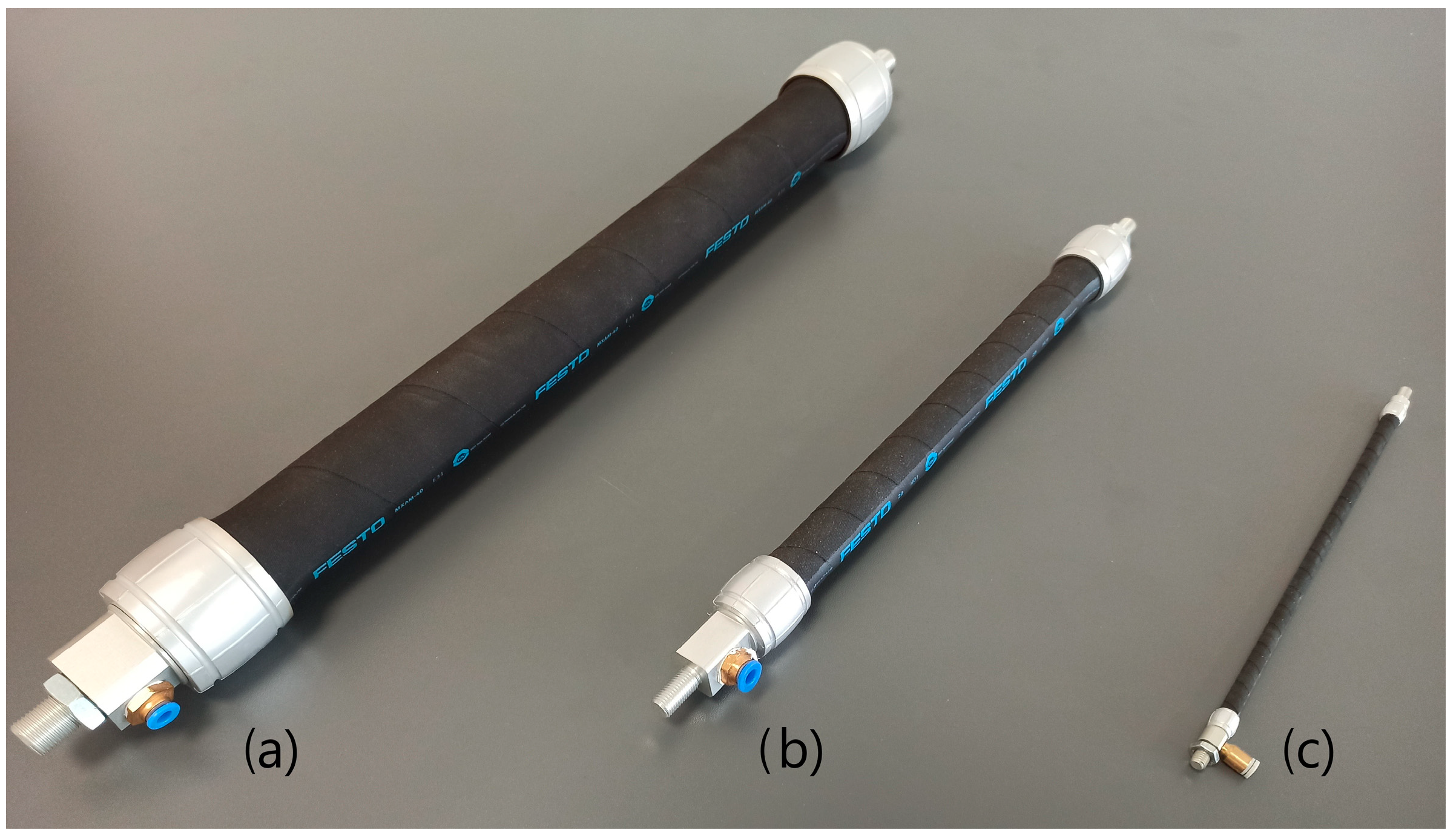
To approximate their characteristics, fluidic muscles from the manufacturer FESTO were chosen. The manufacturer offers them in two variants: the MAS muscle type has a screwed connection, while the DMSP muscle type has press-fitted connections. Figure 1 shows the DMSP type of muscle, which falls into the category of single-acting traction drives. The standard sizes of DMSP muscles offered by the manufacturer are 5, 10, 20, and 40. In this study, three muscles of different sizes were considered: DMSP-40 (Figure 1a), DMSP-20 (Figure 1b), and DMSP-5 (Figure 1c). The designation of the muscles by size is derived from their internal diameter. The nominal muscle length is selectable within a specific range for each muscle size. The force also depends on the size of the muscle. An overview of the technical data of the researched muscles is provided in

Table 3. Overview of the technical data of the selected DMSP muscles [55,56].

Type of Muscle	DMSP-5	DMSP-20	DMSP-40
Internal diameter (mm)	5	20	40
Nominal length (mm)	30 … 1000	60 … 9000	120 … 9000
Max. permissible pretensioning	1% of nominal length	4% of nominal length	5% of nominal length
Max. permissible contraction	20% of nominal length	25% of nominal length	25% of nominal length
Theoretical force (N)	140	1500	6000
Max. additional load (kg)	5	80	250
Operating pressure (bar)	0 … 6	0 … 6	0 … 6
Ambient temperature (°C)	−5 … +60	−5 … +60	−5 … +60

.

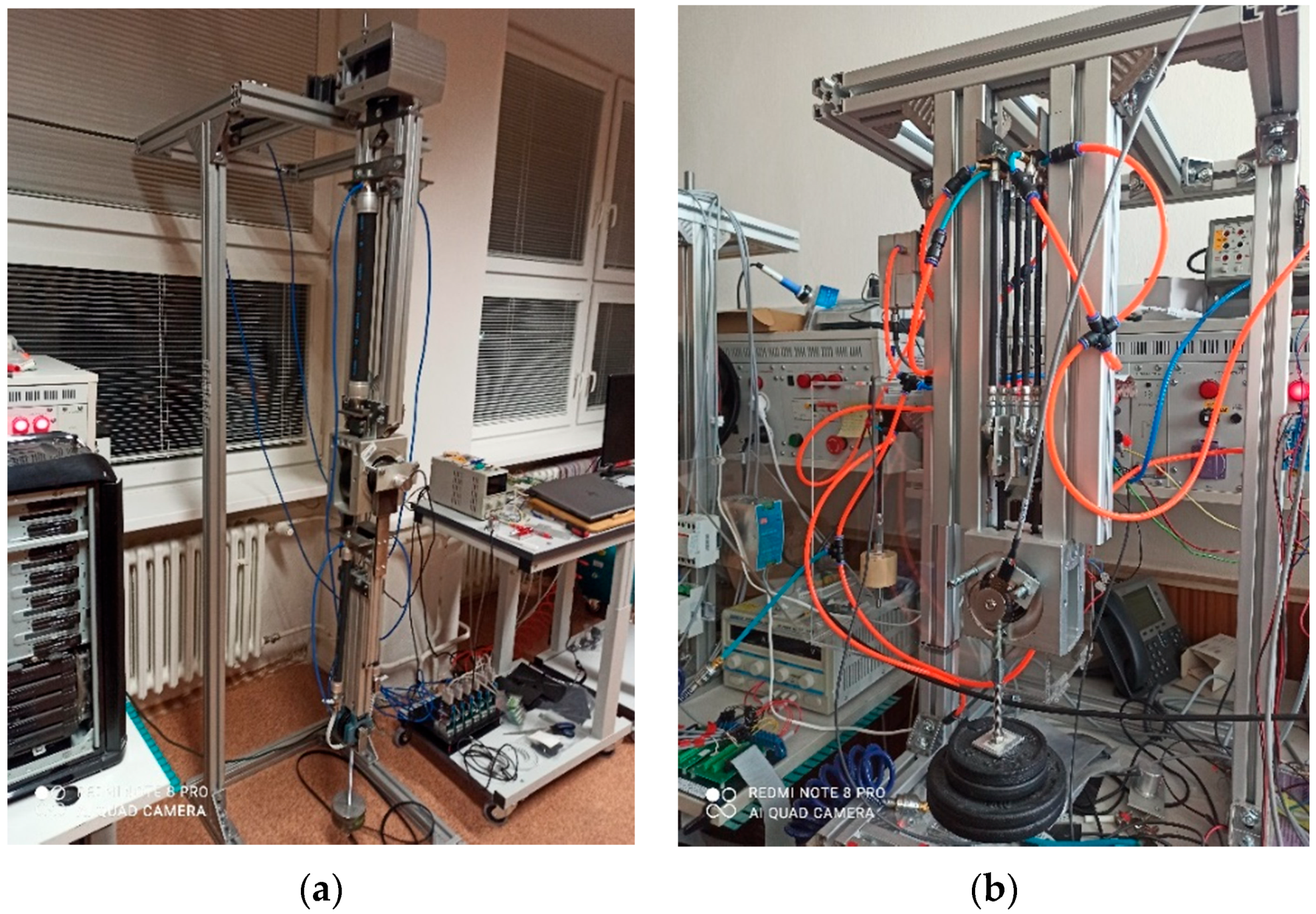
The muscles that were the object of this research were applied at the authors’ workplace in various experimental stands. These devices were assembled to investigate the characteristics and hysteresis of the fluidic muscles, etc.

Figure 2a shows a functional model of a 3-DOF planar robotic arm actuated with DMSP-20 (one pair of FESTO DMSP 20-250N-RM-CM) and DMSP-40 (one pair of FESTO DMSP 40-400N-RM-CM and one pair of FESTO DMSP 20-400N-RM-CM) fluidic muscles. The structure of the manipulator is composed of aluminum profiles, which allow modification of the structure (e.g., in case of the need to shorten/extend one of the arms). Rotational movement is achieved by the antagonistic engagement of three pairs of muscles, joints, and the gear belt subsystem. Electronic pressure regulators (MATRIX ERP50) regulate the pressure in the muscles, which also include pressure sensors. MATLAB/Simulink software is used to control the arm. Control signals are processed with a Humusoft MF624 DAQ PCI card.

A test rig consisting of a multiparallel 1-DOF arm actuated with three pairs of DMSP-5 fluidic muscles is shown in Figure 2b. The rig is made of aluminum profiles and uses six identical muscles with a length of 200 mm (DMSP 5-200N-RM-CM) to actuate a revolute joint (Bosch LF6S drive head with toothed belt and pulley) with a threaded rod arm and a 3 kg payload. The pressure in the muscles is controlled using two proportional pressure regulators with a 0–10 V control signal range (FESTO VPPM-6L-L-1-G18-0L10H-V1P-S1), and pressurized air is generated using a silent compressor (ABAC OS20P-1,5-6RM). The joint angle is sensed using a high-resolution rotary encoder (US Digital E3 with 3600 CPR). All signal processing and generation of control signals is provided by a PC (i7-8750H/8GB) with a DAQ (Humusoft MF644) connected to the computer using a Thunderbolt interface.

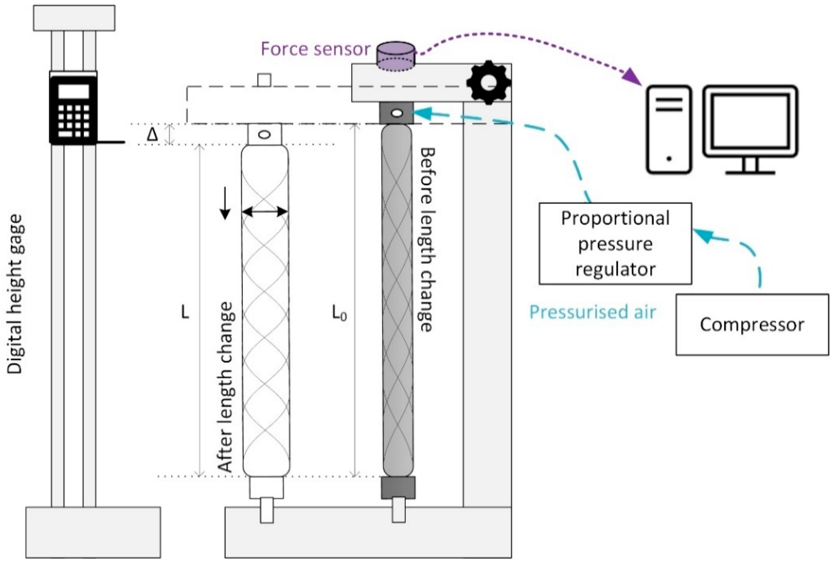
A schematic diagram of the test stand that was used for measuring the characteristics of the DMSP-5 muscle is shown in Figure 3. The test stand was designed to measure the muscle’s static characteristics under isobaric conditions (i.e., with constant pressure). The stand consisted of a structure on which the DMSP-5 muscle was attached (both ends of the muscle were firmly attached to the frame of the structure). Compressed air was let into the muscle by the compressor, which was regulated as needed (1–6 bar, with a step of 0.5 bar) using a proportional pressure regulator. With the help of a sliding mechanism, the required contraction of the muscle was ensured, which was measured using a digital height gauge. Therefore, the input value for the measurement was the required muscle contraction (calculated to the length of the muscle) under constant pressure in the muscle. The output monitored variable was the tensile force of the muscle recorded using the force sensor at a given pressure constant.

4. Approximations of the Muscle Characteristics: Theoretical Background

The following well-known and frequently used models were used to approximate the characteristics (i.e., the forces of FESTO fluidic muscles depending on the muscle contraction and pressure in the muscle):

• MLP (multilayer perceptron network) model;
• SVM (support-vector machine) model;
• ANFIS (adaptive neuro-fuzzy inference system) model;
• Custom (polynomial) model.

The following parts of this chapter describe the basic theoretical premises for the individual models in more detail.

4.1. MLP Model

Since the investigated systems described above represent nonlinear dynamic systems. The first model that was chosen for the approximation of muscle characteristics was the MLP model. The MLP network is one of the most well-known neural network models that allows the classification or approximation of nonlinear functions. The basic task of the network is to transform inputs u_j (number of inputs = p) into outputs y with the help of activation functions ϕ_i—most often hyperbolic tangents (Equation (1)) or logistic functions (Equation (2)) [57,58]:

$$tauh \left(x\right)=\frac{1-exp\left(-2x\right)}{1+exp\left(-2x\right)}$$

(1)

$$logistic \left(x\right)=\frac{1}{1+exp\left(-x\right)}$$

(2)

The architecture consists of a minimum of one hidden layer with a minimum of one neuron called a perceptron (M = the number of perceptrons of the hidden layer), which is subsequently linked to a neuron on the output layer. The hidden layer parameters (hidden layer weight w_ij) are nonlinear in nature and determine the direction and position of the basis functions. Conversely, the output layer parameters (output layer weights w_i) are linear and determine the amplitude of the functions. The output of the MLP network can then be expressed by the following equation [57,58]:

$$y={\displaystyle \sum }_{i=0}^M{w}_i{\varphi }_i\left({\displaystyle \sum }_{j=0}^p{w}_{ij}{u}_j\right)$$

(3)

Derivations of the output y of the MLP network according to the weights of the hidden layer w_ij can be determined by Equation (4), which applies to the weight of the connection between the jth input and the ith neuron of the hidden layer. The function g(x) represents an activation function, e.g., tanh(x). After instituting this form of function into Equation (4), Equation (5) arises. It follows that the activation function ϕ_i is dependent on two parameters, namely, the inputs u_j and the weights of the neurons on the hidden layer w_ij. The mentioned method represents the backpropagation algorithm for determining the gradients of the MLP network according to the weights [57,58].

$$\frac{\partial y}{\partial w_{ij}}=w_{i }\frac{dg\left(x\right)}{dx}{u}_j ; pre u_0=1, i=1\dots M, j=0\dots p$$

(4)

$$\frac{\partial y}{\partial w_{ij}}=w_{i }\left(1-{\varphi }_i^2\right)u_j ; pre u_0=1$$

(5)

4.2. SVM Model

The SVM model is a very popular supervised machine learning algorithm used to solve classification and regression tasks, as it offers the best results in many cases. SVM is a method where the goal of the algorithm is to find a hypersurface that divides the data into classes, but with the condition that these classes are as far apart as possible. If the data can be divided by a linear straight line, the model is a linear SVM. However, if it is necessary to use a nonlinear function for data distribution, the model is a nonlinear SVM, which uses a combination of support vectors with a kernel function.

The method of support vectors is based on the essence of calculating the scalar products of two observations (Equation (6)), while Equation (7) applies to the linear classifier of support vectors [59,60]:

$$\langle x_i,{x_i}^{\prime }\rangle ={{\displaystyle \sum }}_{j=1}^p{x}_{ij}{x}_{i^{\prime }j}$$

(6)

$$f\left(x\right)={\beta }_0+{{\displaystyle \sum }}_{i=1}^n{\alpha }_i\langle x,x_i\rangle$$

(7)

It follows from these equations that n parameters α_i, i = 1, …, n are assumed. To estimate the parameters β₀, α₁, …, α_n, it is necessary to determine the scalar products between all pairs of two observations. However, if these scalar products are replaced by a generalized function that quantifies the similarity of two observations, the linear kernel function (Equation (8)) arises. The task of the kernel function is to transform the data into a higher-dimensional space, where it is possible to find a hypersurface that can divide the data into classes. Within the framework of nonlinear kernel functions, the polynomial kernel (Equation (9)) is known, where d interprets the degree of the polynomial in the form of a whole positive number; along with the radial kernel (Equation (10)), where c is a positive constant [59,60]:

$$K\left(x_i,{x_i}^{\prime }\right)={{\displaystyle \sum }}_{j=1}^p{x}_{ij}{x}_{i^{\prime }j}$$

(8)

$$K\left(x_i,{x_i}^{\prime }\right)={\left(1+{{\displaystyle \sum }}_{j=1}^p{x}_{ij}{x}_{i^{\prime }j}\right)}^d$$

(9)

$$K\langle x_i,{x_i}^{\prime }\rangle =exp\left(-c{{\displaystyle \sum }}_{j=1}^p{\left(x_{ij}-x_{i^{\prime }j}\right)}^2\right)$$

(10)

If a support-vector classifier is combined with a nonlinear kernel, the result is a nonlinear SVM [59,60]:

$$f\left(x\right)={\beta }_0+{{\displaystyle \sum }}_{iϵS}^n{\alpha }_{i}K\left(x,x_i\right)$$

(11)

where S is the set of support vectors.

4.3. ANFIS Model

The third model that was chosen for the approximation of the characteristics was ANFIS. Its name—adaptive neuro-fuzzy inference system—implies that it is a hybrid neuro-fuzzy system, where the fuzzy system is interpreted by a rule of the Takagi–Sugeno type and has the following form:

$$If x_1 is A_1^p and x_2 is A_2^p\dots and x_n is A_n^p than o_p={\alpha }_0^p+{\alpha }_1^p{x}_1+\dots {\alpha }_n^p{x}_n$$

(12)

where x_i is the input linguistic variable, $A_i^p$ is the fuzzy set of the ith input and the pth rule, o_p is the consequent of the pth rule, and ${\alpha }_i^p$ represents the parameters of the consequent.

ANFIS consists of five layers, with each layer playing a different role [61,62]:

LAYER 1—Fuzzification layer: $O_i^1$ is the output of node i of the first layer, while each node is adaptive and has a membership function ${\mu }_{A_i^p}\left(x\right)$, for which Equation (13) applies, where $a_p, b_p, c_p$ is a set of parameters also called premise parameters:

$${\mu }_{A_i^p}\left(x_i\right)=1/\left(1+{\left({\left(\frac{x_i-c_p}{a_p}\right)}^2\right)}^{b_p}\right)$$

(13)

LAYER 2—Operational layer of T-norm: Each node is fixed and corresponds to one rule. The inputs are membership function values combined by T-norm, while the output w_p is the result of all incoming signals:

$$w_p={\mu }_{A_i^p}\left(x_1\right)⨂{\mu }_{A_j^p}\left(x_2\right) i=1,2; j=1,2; p=1,\dots ,4$$

(14)

LAYER 3—Normalization layer: The task is to determine the relative degree of fulfillment of each rule R_p, as follows:

$$\overline{w_p}=\frac{w_p}{{{\displaystyle \sum }}_{p=1}^4{w}_p}$$

(15)

LAYER 4—Layer of consequences: Within this layer, the nodes are connected to exactly one node of the normalization layer. The task of the nodes is to calculate the output of the rule in the form of Equation (16), where the parameters ${\alpha }_i^p$ denote consequents:

$$O_p^4=\overline{w_p}{o}_p=\overline{w_p}\left({\alpha }_0^p+{\alpha }_1^p{x}_1+{\alpha }_2^p{x}_2\right)$$

(16)

LAYER 5—Aggregation layer: The task is to determine the final value of all inputs from the consequent layer:

$$O^5={{\displaystyle \sum }}_{p=1}^4\overline{w_p}\left({\alpha }_0^p+{\alpha }_1^p{x}_1+{\alpha }_2^p{x}_2\right)$$

(17)

5. Results

This chapter presents the results of the approximation of the static characteristics of FESTO muscles using the selected models of computational intelligence and machine learning presented in Section 4. Each of the models was created using one of the toolboxes of MATLAB version 2021b and assessed based on four performance metrics, as presented in Appendix A. In addition to the actual approximation results (also interpreted graphically), the used MATLAB toolboxes are briefly described at the beginning of the chapter, along with the essence of configuring the parameters of the individual models. In addition to using the toolboxes, several commands were used—especially for identifying the values of performance indicators of individual models and the graphical interpretation of model outputs, since individual toolboxes do not provide the same interpretation of outputs.

Depending on the muscle size, different datasets were available, which were subsequently used in creating, training, and testing the models. For the DMSP-20 and DMSP-40 muscles, the data were read from the static characteristics provided by the manufacturer. For the DMSP-40 muscle, the tensile strength of the muscle was read over the entire contraction range (not just the operating range). There was a contraction interval of −5% to 30% with a contraction step of 0.5% for individual pressures (0–6 bar). A total of 497 samples were thus obtained. For the DMSP-20 muscle, the tensile force data were read in the same way for individual pressure values of 0–6 bar, but the contraction interval was from −5% to 27% in steps of 0.5%. A total of 455 samples were obtained. However, the dataset for the DMSP-5 muscle was not read from the manufacturer’s specifications; rather, the data were measured using an experimental stand (Figure 3). Through the measurements, characteristic curves were obtained for pressures in the interval of 1–6 bar with a step of 0.5 bar for contractions in the interval of 0 to 20% with a step of 1%. Measurements were carried out in two stages (i.e., inflating and deflating the muscle). A pair of values was thus obtained for each contraction and pressure, and they were subsequently averaged. There were 11 characteristic curves with a total of 497 samples. The total number of samples for individual muscle dimensions was subsequently redistributed at a ratio of 70/15/15% for the training/validation/testing phases, respectively. The total number of samples and the sampling ratios for individual muscles are summarized in

Table 4. Division ratios for training, validating, and testing the created models.

Type of Muscle	Total Number of Samples	Data Division Ratio %	Sample Division
DMSP-5	231	70/15/15	161/35/35
DMSP-20	455	70/15/15	319/68/68
DMSP-40	497	70/15/15	347/75/75

. Normalization of the data was performed implicitly before further processing within the models.

5.1. Neural Network Fitting and Configuration of the Created MLP Models

The MLP models of the neural network were created in the Neural Network Fitting toolbox, which is included in the machine learning and deep learning toolbox group within the MATLAB program. The advantage of this toolbox is that after importing the data and configuring the basic parameters of the network, it is possible to monitor the architecture of the network, but also to perform training/validation/testing without having to use another MATLAB environment. At the same time, the toolbox provides several options for displaying plots (for example, we monitored error histograms and regression plots).

For each muscle type (i.e., DMSP-5, DMSP-20, and DMSP-40), we created five MLP models according to the number of neurons in the hidden layer (1, 2, 5, 10, or 20). The layer size of these networks was in count 1. The number of parameters was also monitored for the individual created models. The input for the network was a two-row matrix with N samples, where each row represented one input parameter—namely, muscle pressure p and muscle contraction h. The output was a one-row matrix with N samples of the tensile force of muscle F. As a training algorithm, we used the Bayesian regularization algorithm.

5.2. Regression Learner App and Configuration of the Created SVM Models

The SVM models were created in the Regression Learner App which, like the previous toolbox, is classified in MATLAB’s machine learning and deep learning toolbox group. This toolbox serves as a comprehensive tool for the creation and subsequent training and testing of linear and nonlinear regression models (e.g., SVM, trees, neural network models, etc.). If the user is not sure which model is most suitable, they can choose several types of models and monitor their success/error rates based on the RMSE criterion. The results of the models can also be interpreted with different graphs, such as response plots, validation residual plots, or predicted vs. actual plots.

A total of six SVM models were created for each muscle. The individual SVM models differed from one another in the functions used: linear, quadratic, cubic, fine Gaussian, medium Gaussian, and coarse Gaussian. The input of the network was a matrix of size 3xN, where the first and second rows represented the inputs pressure and contraction, while the third row was the output, i.e., the tensile force of the muscle. N represents the number of samples in the given matrix. The toolbox allows the selection of the type of validation: cross-validation, holdout validation, or resubstitution validation. In this study, holdout validation was used. All three phases (i.e., training, validation, and testing) were implemented in the aforementioned toolbox. In addition to performance indicators, it is possible to monitor other parameters of the models in the overviews of the created models, such as kernel scale, bias, etc.

5.3. Neuro-Fuzzy Designer and Configuration of the Created ANFIS Models

The ANFIS models were created in Neuro-Fuzzy Designer, which belongs to the control system design and analysis toolbox group. This toolbox allows for designing, training, and validating ANFIS models by importing input/output training data. After importing the data, it enables the generation of an FIS structure (grid partition or subclustering options). For the membership function (MF), the toolbox provides a choice of settings. For its inputs, it is possible to select the number and type of the MFs. The MF type is chosen for its outputs. At the same time, it allows the structure of the created model to be displayed with inputs/outputs, inputs/outputs of the membership function, and rules. The structure also shows what logical operations are used. Before the actual training, it is necessary to choose the optimization method (hybrid or backpropagation), epochs, and tolerance. During training, the toolbox displays a training error. To test the models, they were exported to the workspace of the MATLAB environment and tested using the command evalfis.

Since there are several options to choose from when creating the FIS structure and configuring the membership function, a total of eight ANFIS models were created.

• The first four models, labeled ANFIS 1–4, had the following features: an FIS structure created by grid partition; 4, 6, 8, and 10 input MFs, and Gaussian type; a constant output MF type; a hybrid optimization method; 0 error tolerance; 10 epochs.
• The other four models, labeled ANFIS 5–8, had the following features: an FIS structure created using grid partition; 4, 6, 8, and 10 input MFs, and Gaussian type; a linear output MF type; a hybrid optimization method; 0 error tolerance; 10 epochs.

As the number of MFs used in the model structure increased, so did the total number of model parameters, as also shown in the overview tables themselves.

5.4. Curve Fitting Toolbox and the Configuration of the Custom Equation Models

Curve Fitting Toolbox is classified in MATLAB’s Math, Statistics, and Optimization section. The toolbox enables the analysis of imported data, finding functions for interpreting the input data (interpolant, lowess, polynomial, or custom equations), plotting curves and surfaces, and evaluating the resulting functions based on several performance metrics (e.g., SSE, R-squared, RMSE, etc.). The toolbox also provides modeling techniques such as smoothing, interpolation, or splines.

To compare the results of the MLP, SVM, and ANFIS models, a simple four-parameter model for the force function of the fluidic muscles was used. The model included the multiplication of two terms: one with the first independent variable (i.e., pressure), and the second with the second-degree polynomial function of the second independent variable (i.e., contraction). The model was named a custom model, taken for purposes of comparison from [63]. The name custom model is related to the Curve Fitting Toolbox used, where the custom equation option was selected in the toolbox when entering the adopted model. This model, commonly applied in the model-based control design of FM-actuated mechanisms mentioned in [63], has the form of Equation (18):

$$f\left(x,y\right)=x \left(a_1{y}^2+a_{2}y+a_3\right)+a_4$$

(18)

The task of the toolbox was to find the values of the coefficients $a_1\dots a_4$ for the specified measured data. Therefore, one custom model was determined for each muscle. Testing of the created models, which each had four parameters, was carried out outside the toolbox environment.

5.5. Approximation of the Characteristics of PAMs: DMSP 40

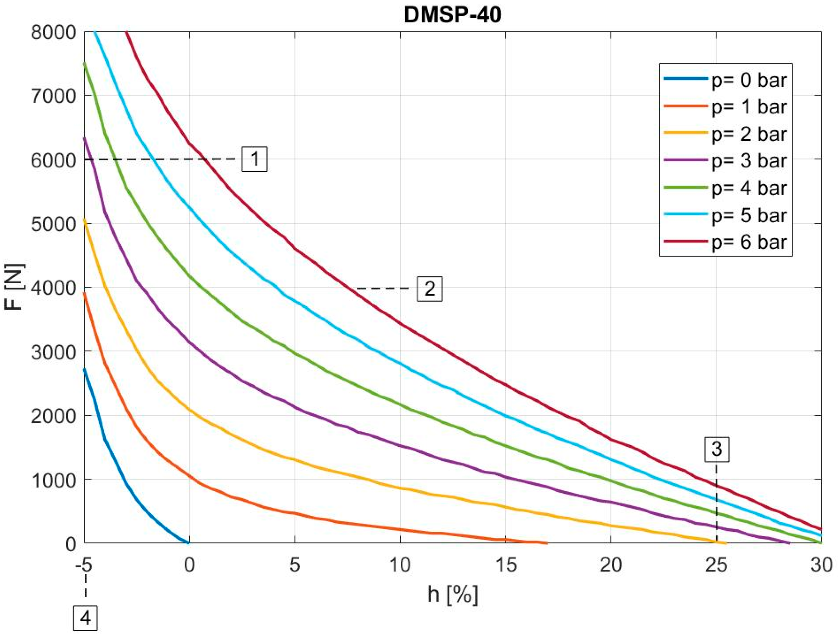
When using muscles, but also when examining them, it is important to know their working ranges. The tensile force of the muscle F (N) is dependent on the contraction of the muscle, but the dependence is nonlinear and is different for different muscles depending on their size. The manufacturer indicates the permissible working range of the muscles and defines it with the help of limit curves.

Figure 4 shows the dependences of tensile force F (N) on contraction h (%) from the nominal muscle length for the DMSP-40 muscle type at constant pressures in the range from 0 to 6 bar, as measured and interpreted by the manufacturer. In the picture, four boundary curves can be seen, where boundary 1 expresses the minimum theoretical force at the maximum operating pressure (6000 N). Boundary 2 represents the maximum operating pressure, which is a value of 6 bar. Boundary 3 expresses the maximum deformation; for the DMSP-40 muscle, this is 25% of the nominal muscle length. Finally, boundary 4 is the maximum pretensioning, which for the DMSP-40 muscle is −5% of the nominal muscle length. The grey area in the graph expresses the permissible operating range for the given muscle.

By recording the data from the force characteristics of a given type of muscle, a set of input/output data used for creating models in MATLAB was created.

Table 5. Overview of the parameters of the created MLP models and performance metrics of the DMSP-40 muscle validation results.

Model	MLP 1	MLP 2	MLP 5	MLP 10	MLP 20
Number of neurons	1	2	5	10	20
Number of parameters	5	9	21	41	81
NRMSE	60.31	62.87	94.77	97.95	90.36
SSE	259,540,000	227,080,000	4,500,700	689,790	15,308,000
AIC	6553.4	6495	4570.2	3678.1	5298.6
SBC	6574.5	6532.9	4658.6	3850.6	5639.5

,

Table 6. Overview of the parameters of the created SVM models and performance metrics of the DMSP-40 muscle validation results.

Model	SVM 1	SVM 2	SVM 3	SVM 4	SVM 5	SVM 6
Kernel scale	0.77162	0.77162	0.77162	0.35	1.4	5.7
Bias	1.45 × 103	1.16 × 103	1.11 × 103	1.67 × 103	2.24 × 103	3.84 × 103
Epsilon	1.76 × 102	1.76 × 102	1.76 × 102	1.76 × 102	1.76 × 102	1.76 × 102
Function	Linear	Quadratic	Cubic	Fine Gaussian	Medium Gaussian	Coarse Gaussian
Alpha	316	137	94	132	73	151
Beta	2	0	0	0	0	0
NRMSE	46.28	54.94	52.61	75.52	61.69	57.32
SSE	4.75 × 108	3.34 × 108	3.70 × 108	9.87 × 107	2.42 × 108	3.00 × 108
AIC	7.48 × 103	6.94 × 103	6.91 × 103	6.33 × 103	6.65 × 103	6.92 × 103
SBC	8.82 × 103	7.52 × 103	7.30 × 103	6.88 × 103	6.96 × 103	7.55 × 103

,

Table 7. Overview of the parameters of the created ANFIS models and performance metrics of the DMSP-40 muscle validation results.

Model	ANFIS 1	ANFIS 2	ANFIS 3	ANFIS 4	ANFIS 5	ANFIS 6	ANFIS 7	ANFIS 8
Input MF	4 4	6 6	8 8	10 10	4 4	6 6	8 8	10 10
MF type	Constant	Constant	Constant	Constant	Linear	Linear	Linear	Linear
Parameters	32	60	96	140	64	132	224	340
NRMSE	63.27	68.99	73.95	77.52	75.65	78.83	81.04	84.09
SSE	2.22 × 108	1.58 × 108	1.12 × 108	8.33 × 107	9.76 × 107	7.38 × 107	5.92 × 107	4.17 × 107
AIC	6.53 × 103	6.42 × 103	6.32 × 103	6.26 × 103	6.19 × 103	6.18 × 103	6.26 × 103	6.31 × 103
SBC	6.67 × 103	6.67 × 103	6.72 × 103	6.85 × 103	6.45 × 103	6.74 × 103	7.20 × 103	7.75 × 103

and

Table 8. Overview of the parameters of the created custom model and performance metrics of the DMSP-40 muscle validation results.

Model Parameters		Metrics
a1	0.2629	NRMSE	53.18
a2	−39.51	SSE	3.6116 × 108
a3	924.9	AIC	6.7156 × 103
a4	94.56	SBC	6.7325 × 103

present overviews of the parameters of the created individual models, along with performance metrics comparing the individual models from the validation phase:

An overview of the results of the MLP models is presented in Table 5, which compares five MLP models that differ from one another in the number of neurons on the hidden layer (and, in turn, the number of parameters). Based on the NRMSE criterion, the model with 10 neurons (marked as MLP 10) was the best model, with 97.95% agreement with the reference model (provided by the manufacturer). From the theoretical starting points presented in the article, it is obvious that for the AIC and SBC metrics the value when the indicator’s value is ideal is unknown. These metrics become important if several models can be compared with one another. It is true that the lower the value of the AIC or SBC, the better the model. The MLP 10 model—which achieved the best evaluation within the NRMSE criterion and, subsequently, in the SSE—had the lowest values of the AIC and SBC indicators. Although this model does not have the lowest number of parameters, it is also not among the most complex models.

• The second type of model that was chosen for approximation was the SVM model. The results of validation based on performance indicators are shown in Table 6. It is obvious that none of the created SVM models could achieve the same results as the best MLP models, since the best-rated model based on the NRMSE criterion (as well as other indicators) was a model with a fine Gaussian function (SVM 4), with 75.52% agreement with the measured data.
• The third type of model was the ANFIS hybrid model. A total of eight ANFIS models were created, which differed in the type of membership function used and the number of function inputs. An overview of the parameters of the created ANFIS models, along with the results of the performance evaluation based on individual indicators after the validation phase for the DMSP-40 muscle, can be seen in Table 7. Based on the NRMSE, the best model was ANFIS 8, with a rate of agreement of 84.09%, with 10 MF inputs and a linear function type. However, this model did not fare the best in the evaluation by the AIC and SBC, as it was the model with the highest number of parameters, which was reflected in the values of these performance indicators. Therefore, the next considered model—with the same type of MF, but a different number of inputs and better AIC and SBC evaluations—could be the ANFIS 6 or ANFIS 5 models. Compared to the best MLP and SVM models, ANFIS ranked between these models in the NRMSE evaluation.
• Since the best models among the MLP, SVM, and ANFIS models had a higher number of parameters, one more model was chosen for comparison: a model with four parameters, interpreted as a custom model. Table 8 shows the identified parameters of the model $a_1\dots a_4$. At the same time, the model was assessed by performance metrics, where the NRMSE indicator achieved 53.18% compliance with the measured data.

5.6. Summary of the Model Results for DMSP-40 (Graphical Interpretation)

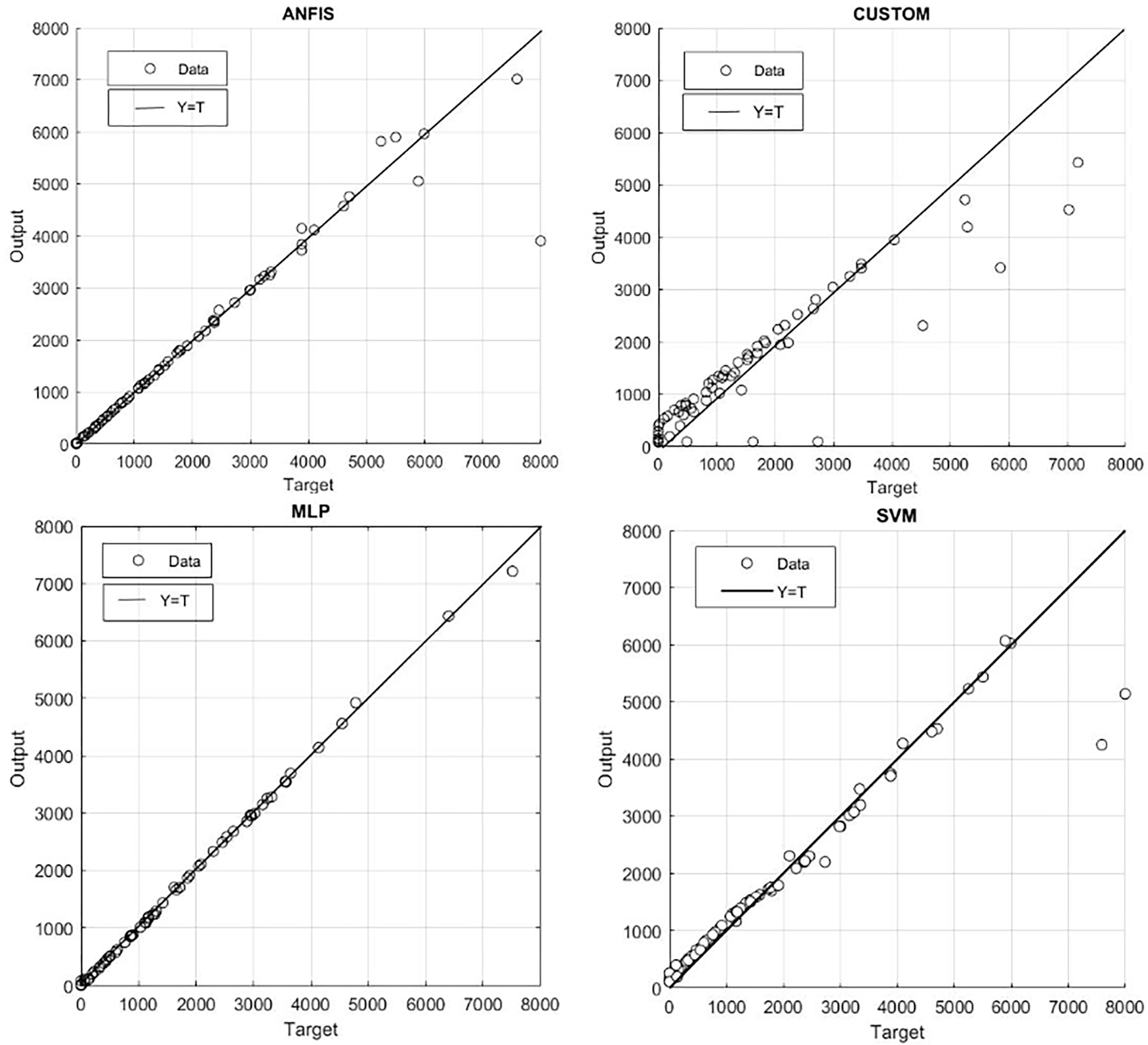
Figure 5 presents a summary of the model results interpreted graphically for the best models of the given groups, where the simulated force is presented as “Output” in correlation with the force measured by FESTO—marked as “Target”—for DMSP-40 within the test phase. The points labeled “Data” are data that were used for the testing phase. The regression line expresses the agreement between the targets and outputs. The more data type values lie on the regression line, the greater the correlation between the outputs and targets. From the results interpreted in Table 5, Table 6, Table 7 and Table 8, it is obvious that within the NRMSE criterion, from best to worst, the first model was the MLP model, followed by the ANFIS, SVM, and custom models. These results can be confirmed by the graphs in Figure 5. The dispersion of values for the custom model in the region of the regression line is considerable, while the dispersion of values for the MLP model is minimal. Within the dispersion of values, it can be assumed that these may be values on the edge or outside the operating range of the muscle. For the custom model, it can be seen that the predicted forces are lower than the measured output. Differences in performance probably result from differences in characteristics in a given area of the operating range.

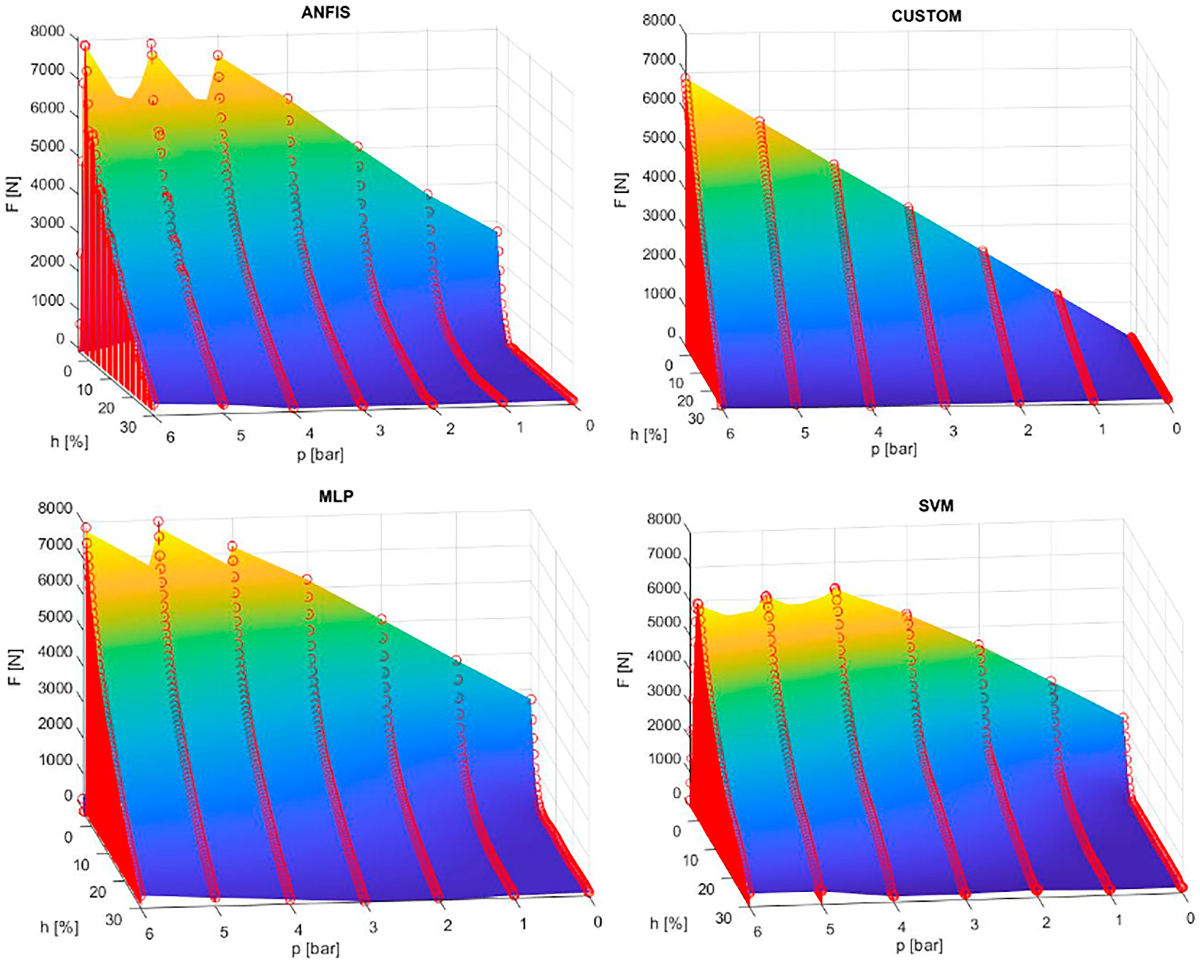
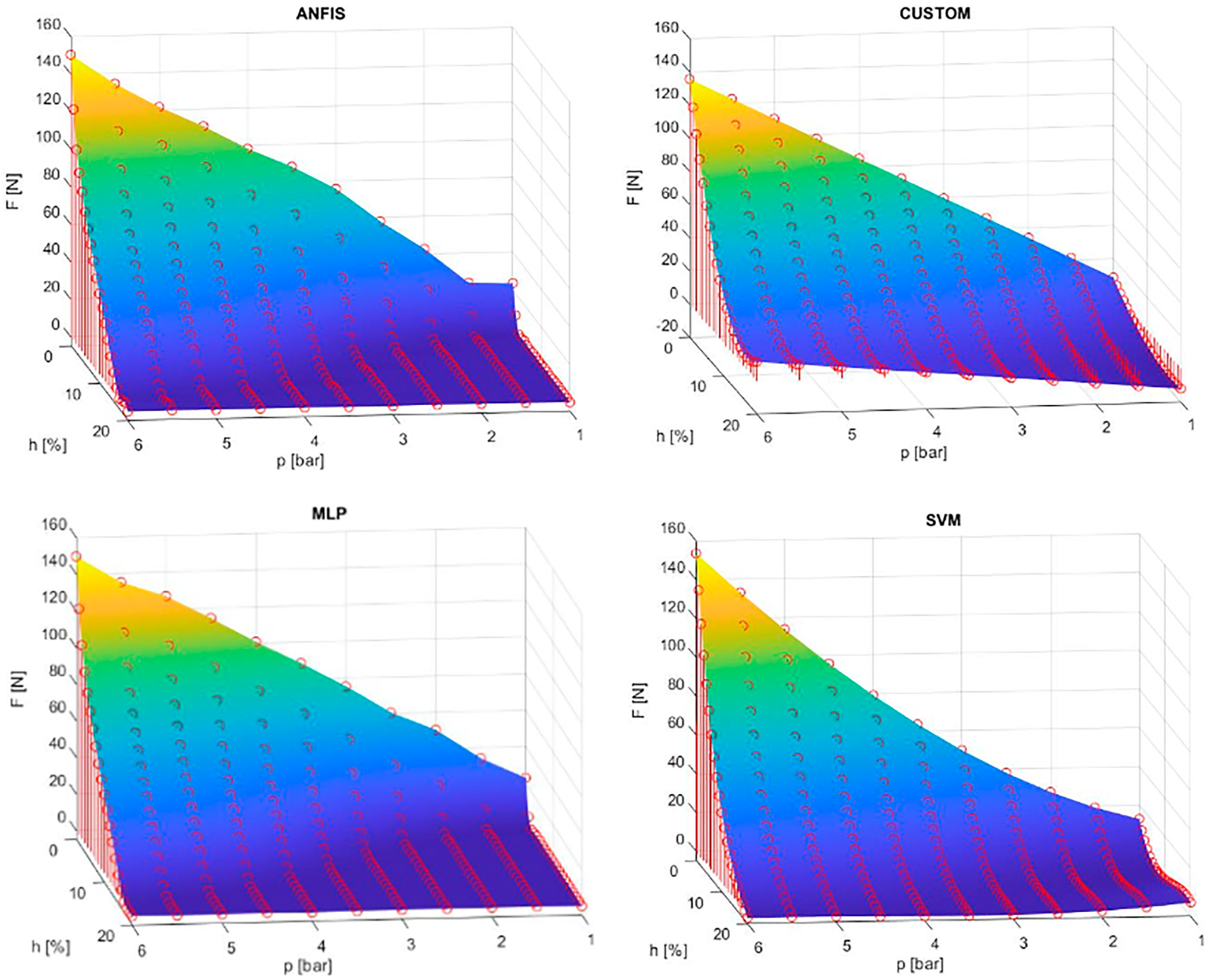
Relations of force, contraction, and pressure approximated by the ANFIS, custom, MLP, and SVM models for the DMSP-40 model are shown in Figure 6. These are 3D surfaces that were created from the simulated outputs of the muscle tensile force parameter models based on the measured values of muscle contractions at constant pressures. As mentioned above, the best model for the DMSP-40 muscle was the MLP model, whose curves and corresponding surface can be seen in the lower left panel of Figure 6.

5.7. Approximation of the Characteristics of PAMs: DMSP 20

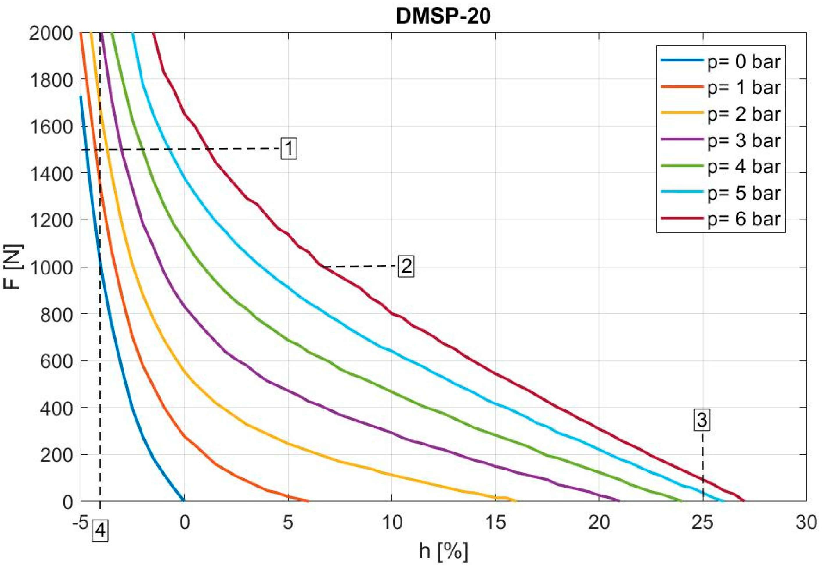
A similar interpretation of the dependence of the tensile force on the muscle contraction also applies to the DMSP-20 muscle, as shown graphically in Figure 7. Just as was the case for DMSP-40 (Figure 4), this is a graphical dependence measured and interpreted by the muscle manufacturer. In the image, it can be seen that the minimum theoretical force at the maximum operating pressure for DMSP-20 is 1500 N (Figure 7; boundary 1). The maximum operating pressure is a value of 6 bar (Figure 7: boundary 2). Moreover, the maximum deformation is the same as for DMSP-40, i.e., 25% of the nominal length of the muscle (Figure 7; boundary 3). However, the maximum pretensioning is somewhat smaller, at −4% of the nominal length of the muscle (Figure 7; boundary 4).

As for DMSP-40, the input/output data from the manufacturer’s operating range for DMSP-20 were read and used to create models, the results of which are interpreted in

Table 9. Overview of the parameters of the created MLP models and performance metrics of the DMSP-20 muscle validation results.

Model	MLP 1	MLP 2	MLP 5	MLP 10	MLP 20
Number of neurons	1	2	5	10	20
Number of parameters	5	9	21	41	81
NRMSE	39.86	66.20	81.62	89.90	88.74
SSE	38,800,000	12,255,000	3,623,100	1,093,700	1,361,200
AIC	5175.9	4659.5	4129.1	3624.1	3803.6
SBC	5196.5	4696.6	4215.6	3793	4137.4

,

Table 10. Overview of the parameters of the created SVM models and performance metrics of the DMSP-20 muscle validation results.

Model	SVM 1	SVM 2	SVM 3	SVM 4	SVM 5	SVM 6
Kernel scale	0.835117	0.835117	0.835117	0.35	1.4	5.7
Bias	331.7927	240.2869	221.3975	367.2308	460.7336	1055.019
Epsilon	44.0972	44.0972	44.0972	44.0972	44.0972	44.0972
Function	Linear	Quadratic	Cubic	Fine Gaussian	Medium Gaussian	Coarse Gaussian
Alpha	319	150	138	145	118	194
Beta	2	0	0	0	0	0
NRMSE	29.62	22.82	19.46	63.45	43.47	30.46
SSE	5.31 × 107	6.39 × 107	6.96 × 107	1.43 × 107	3.43 × 107	5.19 × 107
AIC	5.95 × 103	5.69 × 103	5.71 × 103	5.00 × 103	5.35 × 103	5.69 × 103
SBC	7.27 × 103	6.31 × 103	6.28 × 103	5.60 × 103	5.83 × 103	6.49 × 103

,

Table 11. Overview of the parameters of the created ANFIS models and performance metrics of the DMSP-20 muscle validation results.

Model	ANFIS 1	ANFIS 2	ANFIS 3	ANFIS 4	ANFIS 5	ANFIS 6	ANFIS 7	ANFIS 8
Input MF	4 4	6 6	8 8	10 10	4 4	6 6	8 8	10 10
MF type	Constant	Constant	Constant	Constant	Linear	Linear	Linear	Linear
Parameters	32	60	96	140	64	132	224	340
NRMSE	44.19	55.08	57.90	59.70	60.80	64.76	65.74	65.41
SSE	3.34 × 107	2.16 × 107	1.90 × 107	1.74 × 107	1.71 × 107	1.33 × 107	1.26 × 107	1.28 × 107
AIC	5.16 × 103	5.22 × 103	5.29 × 103	5.38 × 103	5.23 × 103	5.36 × 103	5.55 × 103	5.78 × 103
SBC	5.29 × 103	5.47 × 103	5.69 × 103	5.95 × 103	5.49 × 103	5.91 × 103	6.47 × 103	7.18 × 103

and

Table 12. Overview of the parameters of the created custom model and performance metrics of the DMSP-20 muscle validation results.

Model Parameters		Metrics
a1	−0.1398	NRMSE	20.52
a2	−4.77	SSE	6.7771 × 107
a3	182.7	AIC	5.4277 × 103
a4	77.43	SBC	5.4441 × 103

:

• Table 9 contains the resulting performance indicators for five MLP models that were modeled under the same conditions as the MLP models for the DMSP-40 muscle. Not only within the NRMSE criterion, but also within the SSE, AIC, and SBC indicators, the MLP 10 model with 10 neurons and an NRMSE value of 89.90% agreement with the reference model emerged as the best model.
• An overview of the parameters and results of the SVM models for the DMSP-20 muscle can be seen in Table 10. Among the total of six models created, the best-rated model based on NRMSE (63.45%) was the SVM 4 model, which interprets the SVM model with the fine Gaussian function. The values of the metrics SSE, AIC, and SBC also had the lowest values compared to the other models. Although this model showed the best results in terms of indicators, compared to the best MLP model it achieved a significantly worse result.
• The best ANFIS model for the DMSP-20 muscle also achieved a similar evaluation within the NRMSE as achieved by the best SVM. As part of the overview of the results in Table 11, it can be seen that the best model was ANFIS 7—a model with eight MF inputs and a linear MF. This model has a higher number of parameters, which corresponds to worse ratings within the AIC and SBC indicators. However, within the NRMSE criterion, it achieved the best rating (65.74%). An alternative to the use of the ANFIS 7 model could be the ANFIS 5 or ANFIS 6 models, which achieve worse results within the NRMSE but are simpler models in terms of their number of parameters.
• Similar to the DMSP-40 muscle, for the DMSP-20 muscle the models with a higher number of parameters emerged as the best in the evaluation. However, the custom model created based on Equation (18) achieved a very low value (only 20.52%) in the evaluation based on the NRMSE criterion. The parameters of the custom model, together with the values of other performance metrics, are listed in Table 12.

5.8. Summary of the Model Results for DMSP-20 (Graphical Interpretation)

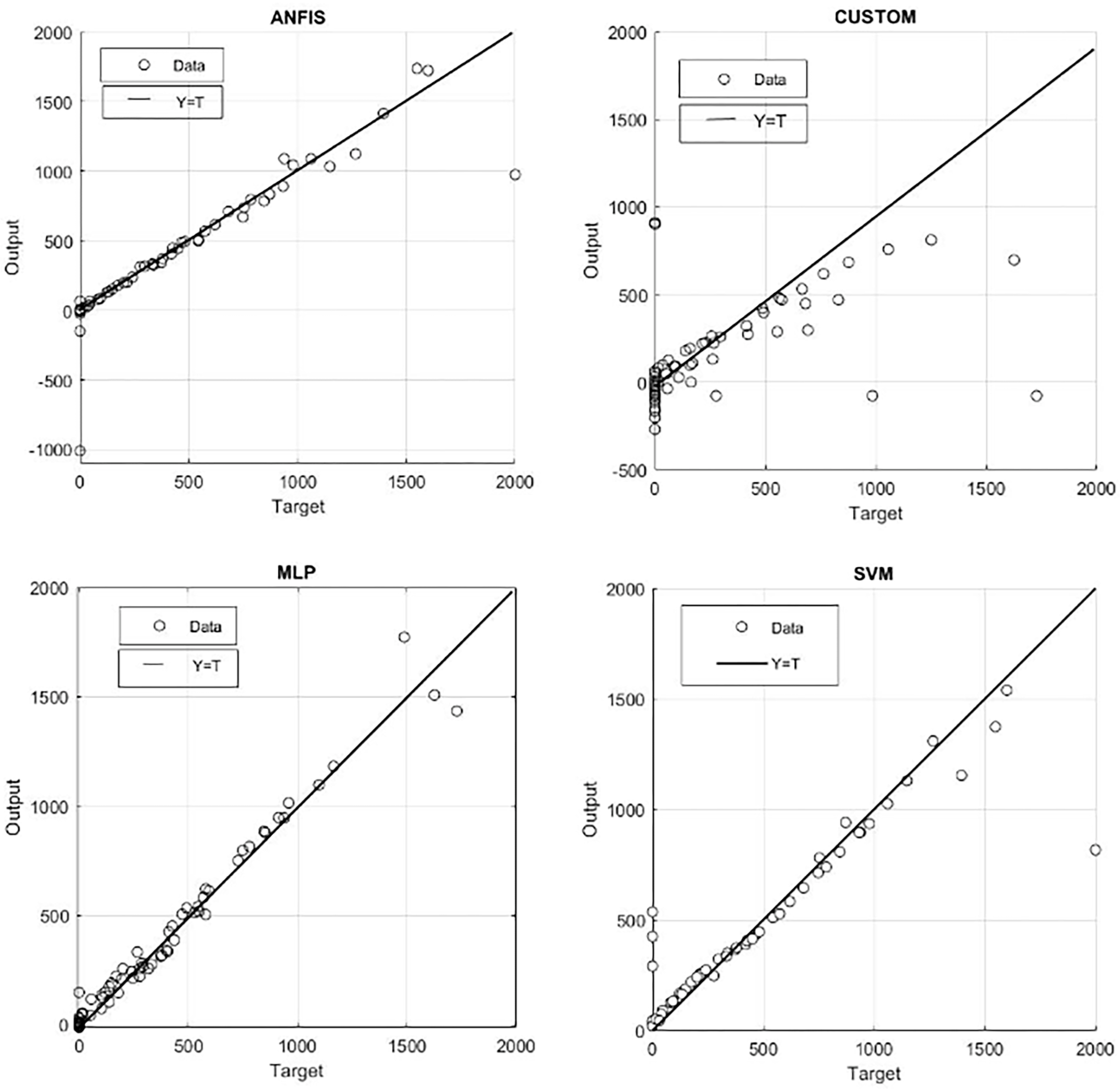
In Figure 8, it is possible to see the simulated force (Output) in correlation with the force measured by FESTO (Target) for DMSP-20 within the test phase. The points labeled “Data” represent data that were used for the testing phase. The regression line expresses the agreement between the target and output. From the results interpreted in the figure, along with those presented in Table 9, Table 10, Table 11 and Table 12, it is clear that the MLP model performed best and the custom model performed the worst (as for the DMPS−40 muscle) within the NRMSE criterion. As with DMSP-40, it can be assumed that the dispersion values may be values on the edge or outside the operating range of the muscle. However, for the custom model, the predicted forces were significantly lower than the measured output. Again, performance differences probably resulted from characteristics in a given area of the operating range.

The obtained simulated outputs of the DMSP-20 muscle’s tensile force depending on the muscle contraction and the pressure in the muscle, which were approximated by the selected models, are graphically displayed for the best individual models in Figure 9. The individual points of the simulated characteristics (red points) create 3D surfaces, and if they are compared with the characteristics given by the manufacturer (Figure 7), it is clear that the MLP model achieved the best approximation. The custom model resulting from the evaluation of performance indicators, as well as from graphical interpretation, was not suitable for approximating the static characteristics of the DMSP-20 muscle.

5.9. Approximation of the Characteristics of PAMs: DMSP-5 Experimental Measured Data

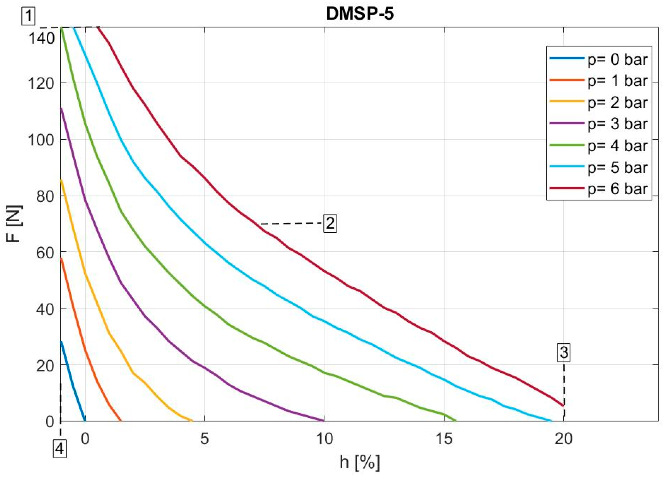
Figure 10 shows the graphical dependence of tensile force on contraction for the DMSP-5 muscle, as reported by the muscle manufacturer. The theoretical force at the maximum operating pressure is much smaller than that of the previous muscles due to its technical parameters (140 N; designation 1 in Figure 10). The maximum operating pressure is the same as for the previous muscles. The maximum contraction is 5% lower (20% of the nominal length of the muscle), and the maximum pretensioning is significantly lower than that of the DMSP-20 and DMSP-40 muscles (−1% of the nominal muscle length).

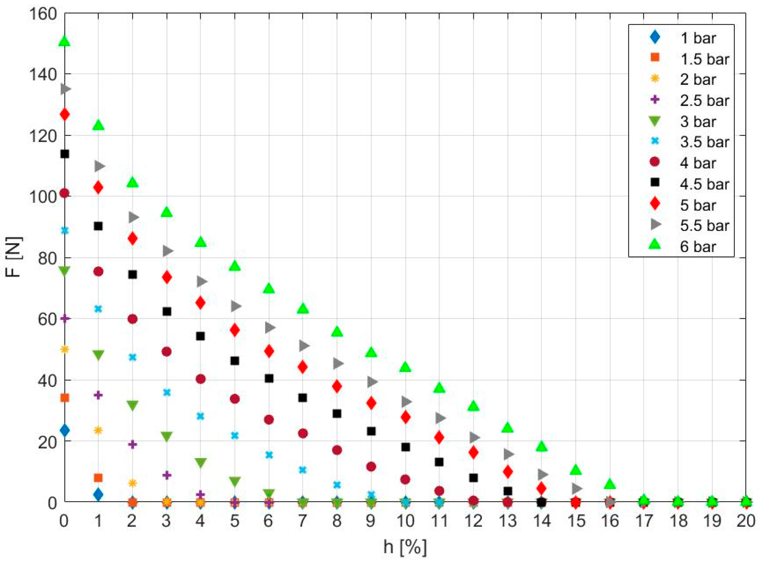
However, data from the manufacturer were not used to approximate the characteristics. Experimental measurements were taken to determine the characteristics of the DMSP-5 muscle on the test device (Figure 3) described in Section 3. Since two sets of measurements were taken for each pressure value (1–6 bar, with a step of 0.5 bar; one measurement at 0–20% contraction; a second measurement at 20–0% contraction), these measurements were subsequently processed and adjusted by averaging the values. The results are the measured static characteristics of the DMSP-5 fluidic muscle, as presented in Figure 11. These measured characteristics subsequently served to create and verify the models.

Table 13. Overview of the parameters of the created MLP models and performance metrics of the DMSP-5 muscle validation results.

Model	MLP 1	MLP 2	MLP 5	MLP 10	MLP 20
Number of neurons	1	2	5	10	20
Number of parameters	5	9	21	41	81
NRMSE	80.91	86.56	95.45	97.11	98.74
SSE	8.32 × 103	4.12 × 103	473.054	190.3272	36.5044
AIC	837.8817	683.7842	207.5791	37.2615	−264.1914
SBC	855.0938	714.766	279.8698	178.4006	14.6444

,

Table 14. Overview of the parameters of the created SVM models and performance metrics of the DMSP-5 muscle validation results.

Model	SVM 1	SVM 2	SVM 3	SVM 4	SVM 5	SVM 6
Kernel scale	1.297189	1.297189	1.297189	0.35	1.4	5.7
Bias	14.64499	5.523659	5.472792	19.65491	31.02986	58.20743
Epsilon	2.112676	2.112676	2.112676	2.112676	2.112676	2.112676
Function	Linear	Quadratic	Cubic	Fine Gaussian	Medium Gaussian	Coarse Gaussian
Alpha	180	138	119	125	70	156
Beta	2	0	0	0	0	0
NRMSE	36.96	76.76	81.93	71.48	80.76	55.03
SSE	9.07 × 104	1.23 × 104	7.46 × 103	1.86 × 104	8.45 × 103	4.62 × 104
AIC	1.74 × 103	1.66 × 103	1.04 × 103	1.26 × 103	971.5456	1.54 × 103
SBC	7.27 × 103	6.31 × 103	6.28 × 103	5.60 × 103	5.83 × 103	6.49 × 103

,

Table 15. Overview of the parameters of the created ANFIS models and performance metrics of the DMSP-5 muscle validation results.

Model	ANFIS 1	ANFIS 2	ANFIS 3	ANFIS 4	ANFIS 5	ANFIS 6	ANFIS 7	ANFIS 8
Input MF	4 4	6 6	8 8	10 10	4 4	6 6	8 8	10 10
MF type	Constant	Constant	Constant	Constant	Linear	Linear	Linear	Linear
Parameters	32	60	96	140	64	132	224	340
NRMSE	81.40	87.28	90.52	93.26	93.71	96.31	86.14	89.97
SSE	7.90 × 103	3.70 × 103	2.05 × 103	1.04 × 103	9.03 × 102	3.10 × 102	4.38 × 103	2.30 × 103
AIC	8.80 × 102	7.60 × 102	6.96 × 102	6.27 × 102	4.43 × 102	3.32 × 102	1.13 × 103	1.21 × 103
SBC	9.90 × 102	9.67 × 102	1.03 × 103	1.11 × 103	6.63 × 102	7.87 × 102	1.90 × 103	2.38 × 103

and

Table 16. Overview of the parameters of the created custom model and performance metrics of the DMSP-5 muscle validation results.

Model Parameters		Metrics
a1	0.07496	NRMSE	72.86
a2	−2.533	SSE	1.6812 × 104
a3	25.39	AIC	998.3944
a4	−16.72	SBC	1.0122 × 103

present the interpretation of the resulting models created for the DMSP-5 muscle:

• Table 13 shows an overview of the parameters and indicators of the MLP models. Compared to the MLP models for DMSP-20 and DMSP-40, based on the NRMSE criterion, the model with 20 neurons (MLP 20) emerged as the best model, with an agreement of 98.74% with the measured data. However, selection based on the SSE, AIC, and SBC metrics would also confirm this selection, as the values of these indicators were the lowest for the model in question.
• The variability in the results of the SVM models for DMSP-5 is visible in the values of the indicators shown in Table 14 (NRMSE ranging from 36.96% to 81.93%). The best model reached an NRMSE of 81.93% using a cubic function (SVM 3). If the best model was chosen based on the SSE, the choice would be the same. However, a change would occur based on the AIC and SBC, when the SVM 5 model with the medium Gaussian function and an NRMSE value of 80.76% would also be a suitable candidate.
• The ANFIS models created and tested for the DMSP-5 muscle achieved much better results compared to the ANFIS models for DMSP-20 and DMSP-40. Moreover, in the comparison of the created models, the results of the NRMSE evaluation for the best ANFIS model (NRMSE = 96.31%) were similar to those of the best MLP model (NRMSE = 98.74%). In Table 15, it can be seen that the best ANFIS model was the ANFIS 6 model, which contains 6 MF inputs and a linear MF. The number of parameters in this model is not the lowest, but at the same time, it does not belong to the group of models with the highest number of parameters. This model achieved the best values in almost all indicators.
• The last approximated function of the static characteristics of the DMSP-5 muscle based on the measured data was a custom model; the transcription of the general equation is identical to Equation (18), and the values of the model parameters are summarized in Table 16. Within the framework of the custom models created for individual muscles, they achieved the highest rating for NRMSE (72.86%). Nevertheless, their results were not comparable with those of the models listed above.

5.10. Summary of the Model Results for DMSP-5 (Graphical Interpretation)

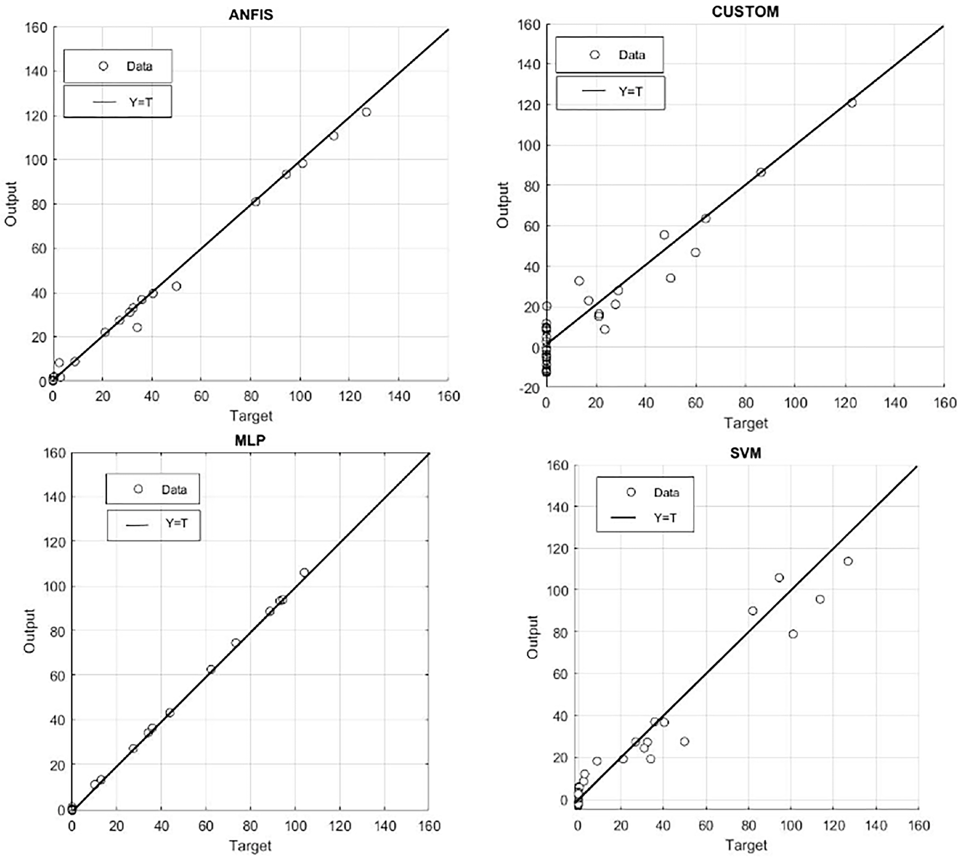
Figure 12 shows an overview of the force simulated (Output) by the ANFIS, custom, MLP, and SVM models in correlation with the force measured (Target) for DMSP-5 in the test phase. From the graphs selected for the best models, it is possible to confirm what was presented in Table 13, Table 14, Table 15 and Table 16, i.e., that the best model for approximating static characteristics based on the NRMSE evaluation criterion is the MLP model. At the same time, the largest dispersion of values around the regression line (and, thus, the worst model) is the custom model.

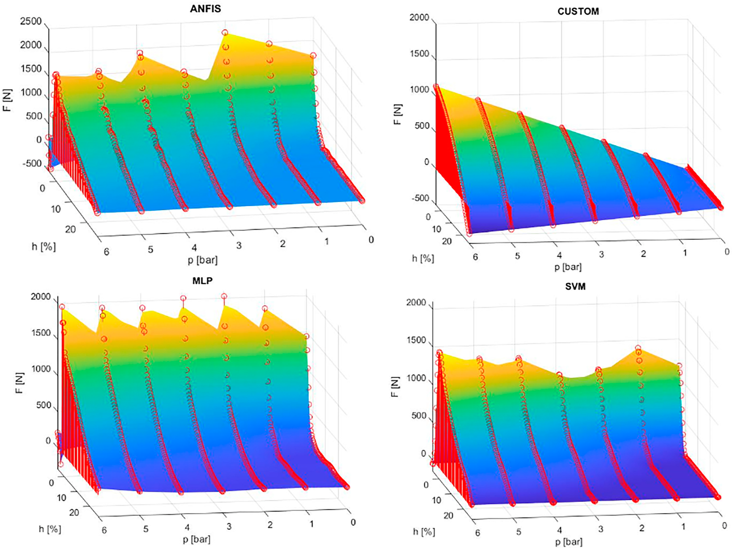
The static characteristics of the DMSP-5 muscle approximated by the best models, along with their created 3D surfaces, can be seen in Figure 13. From the measured characteristics shown in Figure 11—which were used to create the models and, subsequently, to compare their outputs—it is obvious that the maximum tensile force at a pressure of 6 bar should reach 150 N. However, from the graphs shown in Figure 13, it can be seen that the custom model is not capable of approximating the given value; therefore, the custom model was the worst among the individual evaluation models (Table 13, Table 14, Table 15 and Table 16). On the other hand, the curves of the MLP and ANFIS models are very similar and almost identical to the measured output, as proven by the values of the NRMSE criterion.

6. Summary and Discussion

This final section contains a summary of the results together with their discussion and is divided into two parts: The first part summarizes the results of the approximation models for the individual muscles, always choosing the best from a given group of models. The results as described and graphically interpreted in Figure 14, Figure 15 and Figure 16 compare the models’ outputs with the force measured for the individual muscles. This section is followed by a discussion of the results based on the best models according to their correspondence with the measured data and based on their complexity (i.e., number of parameters). The discussion also summarizes the results of the models of all architectures for each of the modeled muscle types using selected performance metrics, which are interpreted graphically in the form of boxplots.

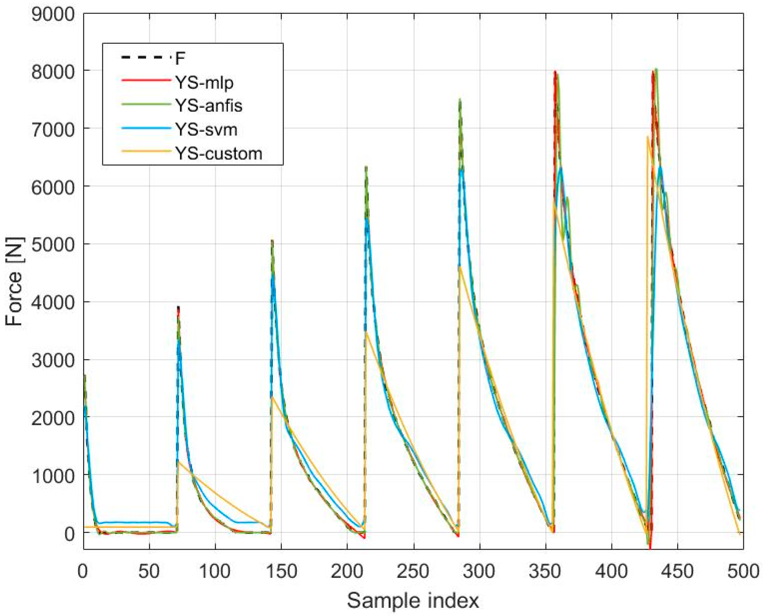
The most relevant graphical overview of the model outputs for the DMSP-40 muscle is presented in Figure 14, which summarizes all of the outputs of the best models in one graph together with the measured data. The measured tensile force is indicated by a black dashed line labeled F. The outputs of the individual models are shown by solid colored lines:

• MLP model with 10 neurons and an NRMSE value of 97.95% (red line, marked as YS-mlp);
• ANFIS model with 10 MF inputs and a linear MF, with an NRMSE value of 84.09% (green line, marked as YS-anfis);
• SVM model with a fine Gaussian function and an NRMSE value of 75.52% (blue line, marked as YS-svm);
• Custom model with an NRMSE value of 53.18% (yellow line, marked as YS-custom).

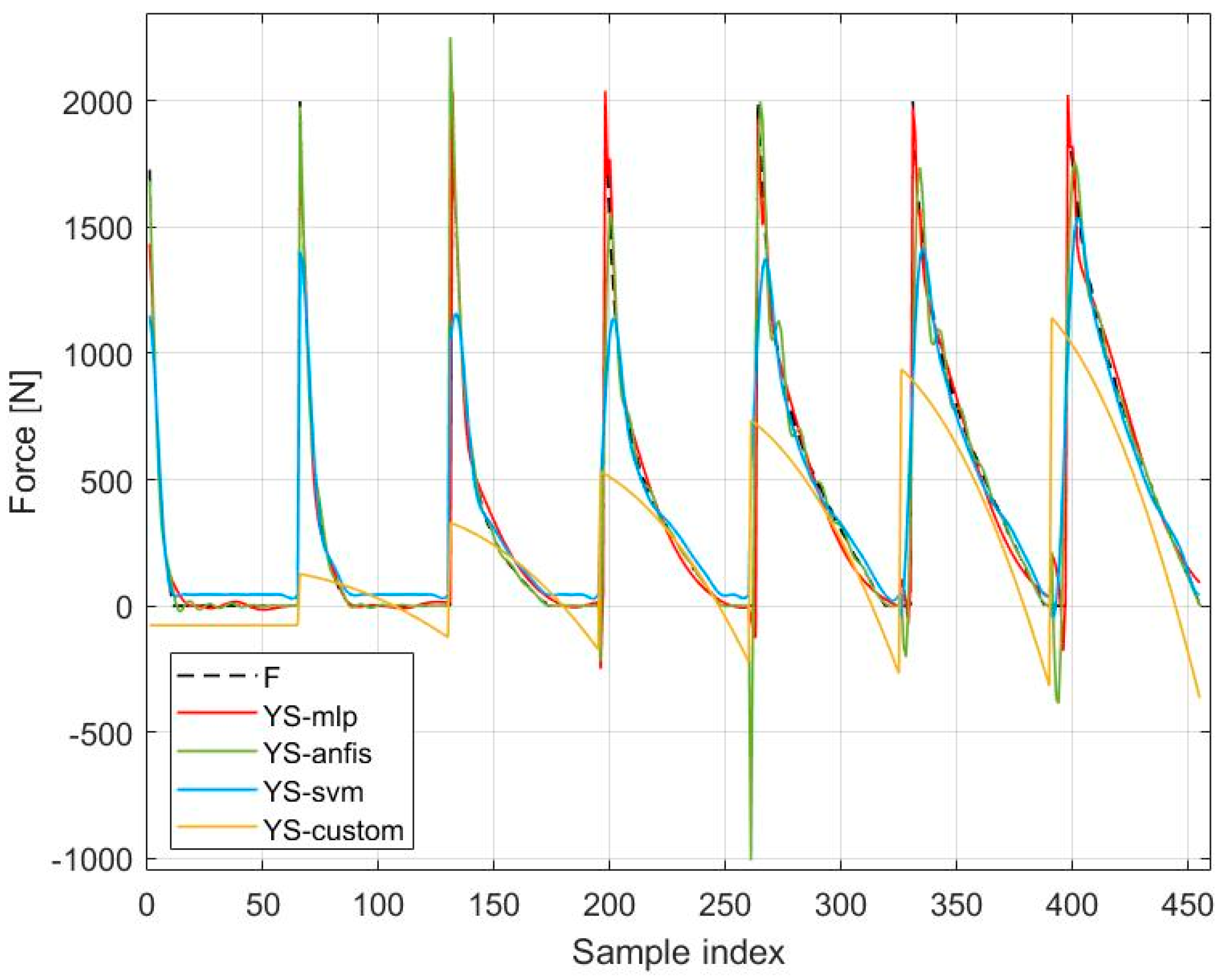
An overview of the model outputs, summarizing all of the outputs of the best models in one graph together with the measured data for the DMSP-20 muscle, is shown in Figure 15. The measured tensile force is indicated by the black dashed line marked F. The outputs of the individual models are shown by solid colored lines:

• MLP model with 10 neurons and an NRMSE value of 89.90% (red line, marked as YS-mlp);
• ANFIS model with 8 MF inputs and a linear MF, with an NRMSE value of 65.74% (green line, marked as YS-anfis);
• SVM model with a fine Gaussian function and an NRMSE value of 63.45% (blue line, marked as YS-svm);
• Custom model with an NRMSE value of 20.52% (yellow line, marked as YS-custom).

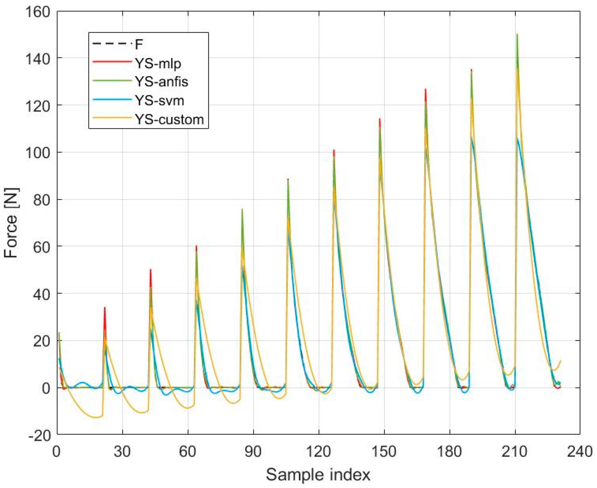
A comparison of the outputs of the best models in one graph, together with the experimentally obtained data for the DMSP-5 muscle, is shown in Figure 16. The measured tensile force is indicated by a black dashed line labeled F. The outputs of the individual models are shown by solid colored lines:

• MLP model with 20 neurons and an NRMSE value of 98.74% (red line, marked as YS-mlp);
• ANFIS model with 6 MF inputs and a linear MF, with an NRMSE value of 96.31% (green line, marked as YS-anfis);
• SVM model with a cubic function and an NRMSE value of 81.93% (blue line, marked as YS-svm);
• Custom model with an NRMSE value of 72.86% (yellow line, marked as YS-custom).

Taking into account the results of the measured force characteristics of the investigated muscle types (either supplied by the muscle manufacturer or determined during the experiments), it can be observed that the function has a similar form but with different scaling. However, simple scaling of the output of a single model trained with the data for one of the muscle diameters would not be sufficient to obtain a good performance when higher accuracy is required. The 3D plots of the function reveal two important areas that manifest themselves differently when using various types of muscle force function approximators. One of the areas is the area of zero-force values, which increases with the decrease in the value of muscle pressure. The other area includes the area of non-zero muscle force, i.e., the area where a muscle actually performs useful work and generates force. It is noteworthy that in the case of measurements carried out for DMSP-5, the distribution of the data was denser for set pressures because of the lower pressure step (50 kPa, compared to 100 kPa for the characteristics given by the manufacturer). In addition, the mean curves of two directions of length changes were used; therefore, the hysteresis of the force function was not considered.

As shown in the results for model performance, the area of zero force appears to be more demanding in terms of the required flexibility of the model for achieving higher accuracy. As a result of this, the performance of the simple custom model with four parameters is significantly reduced compared to the other models. While the inaccuracies of the muscle force model approximators in the zero-force area caused by the output reaching negative values could be handled using the saturation function with a lower bound of zero, this solution would not help for the output errors above zero. Moreover, the regression plots for test data shown in Figure 12 illustrate that both the SVM and custom models also have inferior performance in the area of higher force. Even though the approximation capabilities of ANFIS and MLP are naturally expected to be more powerful due to their higher numbers of parameters, it is important to obtain parsimonious models where the balance of model complexity and performance is taken into consideration. These can be compared using the AIC and SBC performance metrics which, based on the results, still favor the MLP models.

In

Table 17. Summary of the best results for each type of DMSP fluidic muscle.

Metrics	DMSP-40	DMSP-20	DMSP-5
	MLP 10	MLP 10	MLP 20
AIC	3678.1	3624.1	−264.1914
SBC	3850.6	3793	14.6444
NRMSE	97.95%	89.90%	98.74%

, which summarizes the best results for each type of DMSP fluidic muscle, it is clear that the MLP model prevails as the best within the individual muscles. Nevertheless, let us analyze these results:

• For the DMSP-40 muscle, the MLP 10 model achieved an AIC of 3678.1 and an SBC of 3850.6. The other models that approached these values were also from the MLP group. The SVM models started at AIC 6330 and SBC 6880 (SVM 4). The ANFIS models started at similar values—AIC 6190 and SBC 6450 (ANFIS 5). The custom model achieved values in these metrics that ranked it among the models with weaker results.
• A similar scenario occurred for the DMSP-20 muscle, with the best AIC and SBC values of 3624.1 and 3793, respectively, for the 10-neuron MLP. Although the AIC and SBC values of the best model were similar to those for the DMSP-40 muscle, at the same time, the models that approached the best results were also from the group of MLP models, with only one change. The SVM, ANFIS, and custom models achieved lower values in the AIC and SBC parameters than for the DMSP-40 muscle. For example, the best SVM model started at AIC 5000 and SBC 5600 (SVM 4), while the best ANFIS model started at AIC 5160 and SBC 5290 (ANFIS 1). The values of these two metrics for the custom model were around 5400.
• However, the most fundamental difference in the AIC and SBC metrics was observed for the DMSP-5 muscle. The metric values of the best MLP model, with 20 neurons, can be seen in Table 17. However, interesting results were also achieved by the ANFIS 6 model, with AIC 332 and SBC 787, as well as by the custom model, where the AIC reached 998.3944 and the SBC reached 1012.2. The best SVM model (SVM 5) started with AIC and SBC values of 971.5456 and 5830, respectively.

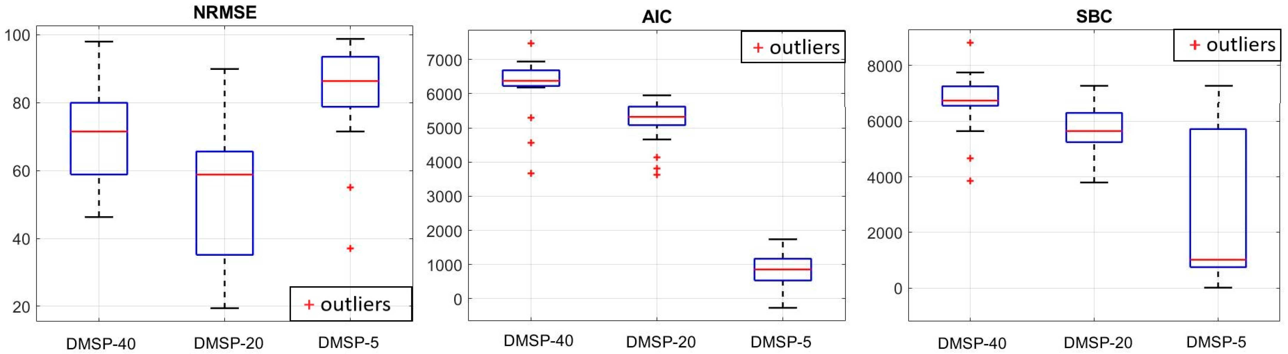
It is also interesting to generalize the performance of the models using the selected performance metrics for all muscle types in question (Figure 17 and Table 17). Generally, we were interested in the best results for the approximation of muscle force function. The boxplots in Figure 17 allow the capabilities of the selected architectures of the approximators to be evaluated. However, it must be noted that only the NRMSE metric includes normalization and, thus, makes the results comparable between the muscle types. The highest median values of the NRMSE metric, recorded for DMSP-5, were probably caused by the different method of obtaining data, as well as the slightly increased number of data samples. On the other hand, the best-performing function approximators had fit values in the order of 90% (Table 17). The AIC metrics show similar ranges of their 25th and 75th percentiles, but the unnormalized form causes different placement of their respective boxplots on the y-axis. In terms of model parsimony, the AIC and SBC criteria are more important because of their reflection of the complexity/fit balance. The boxplots of the AIC criterion also confirm that several models performed much better compared to others (i.e., low-value outliers). This applied to the MLP models, which dominated the other model architectures for this type of function.

It appears probable that the sigmoid activation function is especially suited for the shape of a DMSP muscle force function and can obtain a good approximation with the best complexity/fit balance, as reflected in the values of AIC. The summary results shown in Table 17 allow the best model approximator to be determined—in all three cases, it is the MLP architecture, with the 10-neuron structure for DMSP-20 and DMSP-40, and with the 20-neuron structure for DMSP-5. However, the difference in NRMSE between MLP-10 and MLP-20 is roughly 1.5%, which makes MLP-10 possibly the best choice for the approximation of DMSP muscles’ force function.

Table 18. Performance comparison of several state-of-art models with the best ML model.

Model	Analytical	Maximum Force	Exponential Function	Polynomial Function	MLP 10
	[47,64]	[47,65]	[47,49]	[47,48]	−
Number of parameters	5	8	6	21	41
Number of samples	417	417	417	417	455
RMSE	81.22	473	209.2	164.5	49.02791
SSE	2,784,000	93,740,000	18,420,000	10,990,000	1,093,700
AIC	3682.2	5154.7	4472.2	4286.8	3624.1
SBC	3702.4	5186.9	4496.4	4371.5	3793

shows the comparison of the relevant metrics for the best-performing model in this work (i.e., MLP10 for DMSP-20, which was the only muscle used in other references) with four other models used in other works.

It must be noted that the number of data points was not available and had to be estimated based on the used metrics (it was determined to be 417). It can be observed that the value of RMSE was the lowest for the case of MLP10; of course, as expected in the case of ML models, this was achieved with a higher number of parameters. Nevertheless, the value of AIC, which takes the balance between model accuracy and complexity into account, was still the lowest. This suggests that the high flexibility of ML models might be rewarded with a sufficiently high increase in accuracy to retain the beneficial balance of accuracy/complexity in the resulting models. In consequence, when high accuracy is of interest (e.g., in simulation models used for optimization or verification), the parsimonious ML models can be useful. In addition, the high flexibility of these models allows researchers to vary their structure, include additional inputs easily, and also achieve very high accuracies that other models might not be capable of [66].

The algorithms for training the ML models were sequential minimal optimization for the SVM models, a hybrid method (i.e., LS and backpropagation) for training the ANFIS models, and the Levenberg–Marquardt algorithm for training the MLP models. The SMO algorithm for SVM training is said to reduce the time complexity to O(n) [67]. Hybrid training of ANFIS has a dominant time complexity of O(n²) [68], while LM training of MLP has a time complexity of O(n³) [69]. It should be noted that these are the time complexities for the training of the models, which is expected to be carried out offline if their use in the simulation of PAM-driven mechanisms is assumed.

7. Conclusions

The aim of this research was to approximate the static characteristics of FESTO DMSP-type fluidic muscles using selected methods of computational intelligence and machine learning. The study, which analyzed the results of the experiments described in this article, can be divided into the following stages:

• Reading of the static characteristics of the dependence of the tensile strength of the DMSP-20 and DMSP-40 muscles upon muscle contraction at constant pressures.
• Experimental acquisition of a representative dataset on the dependence of the tensile force of the DMSP-5 muscle on the contraction of the muscle at constant pressures on the testing device developed by the authors.
• Creation of MLP, SVM, ANFIS, and custom models in MATLAB and associated toolboxes for individual types of muscles.
• Testing of the trained models on an independent dataset and performance evaluation of model outputs compared with real outputs, based on the performance indicators NRMSE, SSE, AIC, and SBC.

Based on the results, which are described in detail in the Results and Discussion section, it is obvious that the functions of the force characteristics of the muscles have a similar form, but with different scaling; therefore, each type of muscle mentioned in this article must be considered separately. Nevertheless, the results can be summarized in the following findings:

• The flexibility of the created models was lower in the area of zero force (maximum contraction values), which reduced the performance of the models.
• In general, models from the MLP group achieved the best results in all performance metrics.
• The sigmoid activation function appears to be a suitable candidate for the muscle force function of the DMSP muscles; not only can it approximate with high values of fit, it also offers a compromise in terms of the complexity-to-fit ratio of the model.
• Given that the aim of this article was to find models with not only high performance but also a good complexity/fit balance, the best model based on the results appears to be the MLP with 10 neurons for each of the mentioned types of DMSP muscle from the manufacturer FESTO.

Considering the above information, in the future, we would like to improve the best models—whose performance is reduced due to low flexibility in the region of zero force (negative values)—by using a saturation function with a lower limit defined at zero. By increasing the flexibility of models in the field of zero force and, at the same time, using the information and knowledge that we acquired during the processing of this article, we wish to ensure the optimal conditions for the creation of models of the mechanisms described in this article and to which DMSP muscles are applied.