

Logarithm-Based Methods for Interpolating Quaternion Time Series


Abstract
1. Introduction
1.1. Relating Rotations across Parent/Child Pairs
1.2. A Brief Introduction to Quaternions
1.3. Slerp and Squad
1.4. Renormalized Quaternion Bezier (Rqbez) Interpolation
1.5. Logarithmic Quaternion Interpolation (Lqi)
1.6. The Ambiguity of the Quaternion Logarithm
| Algorithm 1: Recovering a axis-angle series for logarithmic interpolation |
 |
1.7. Modified Logarithmic Quaternion Interpolation (Mlqi)
2. Results and Discussion
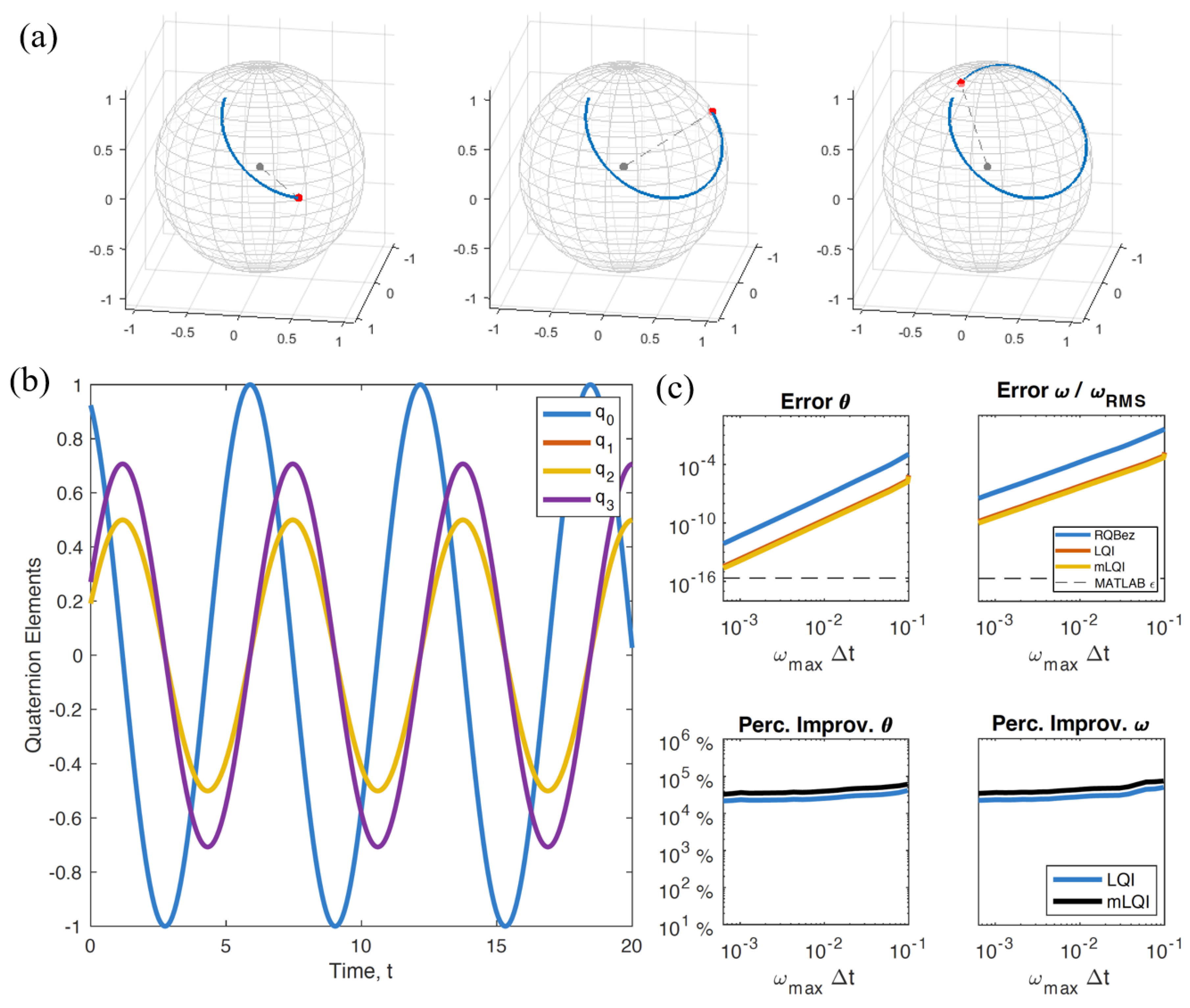
2.1. Example 1: Simple Rotation in the Angle
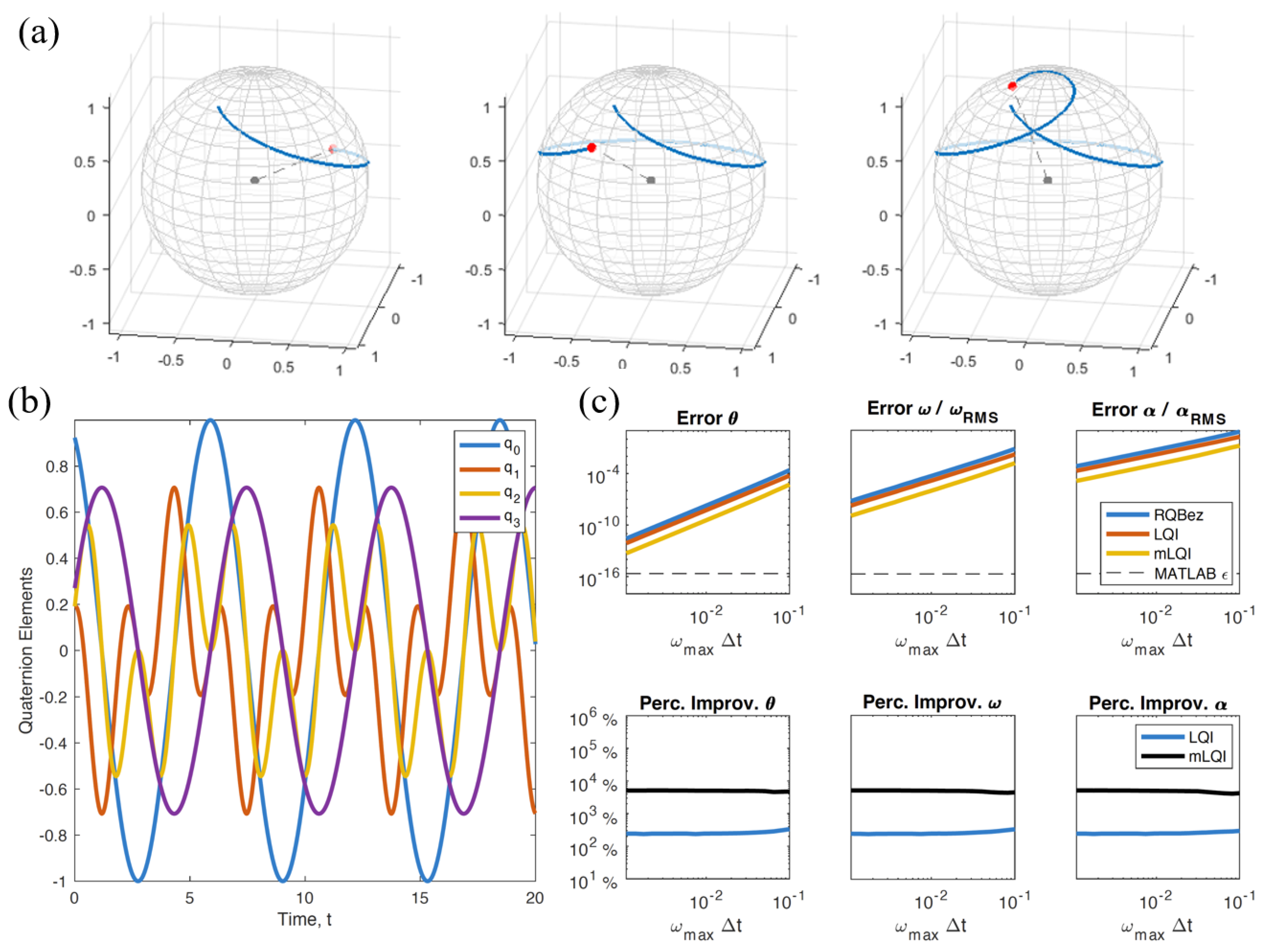
2.2. Example 2: Simple Mixed Rotation
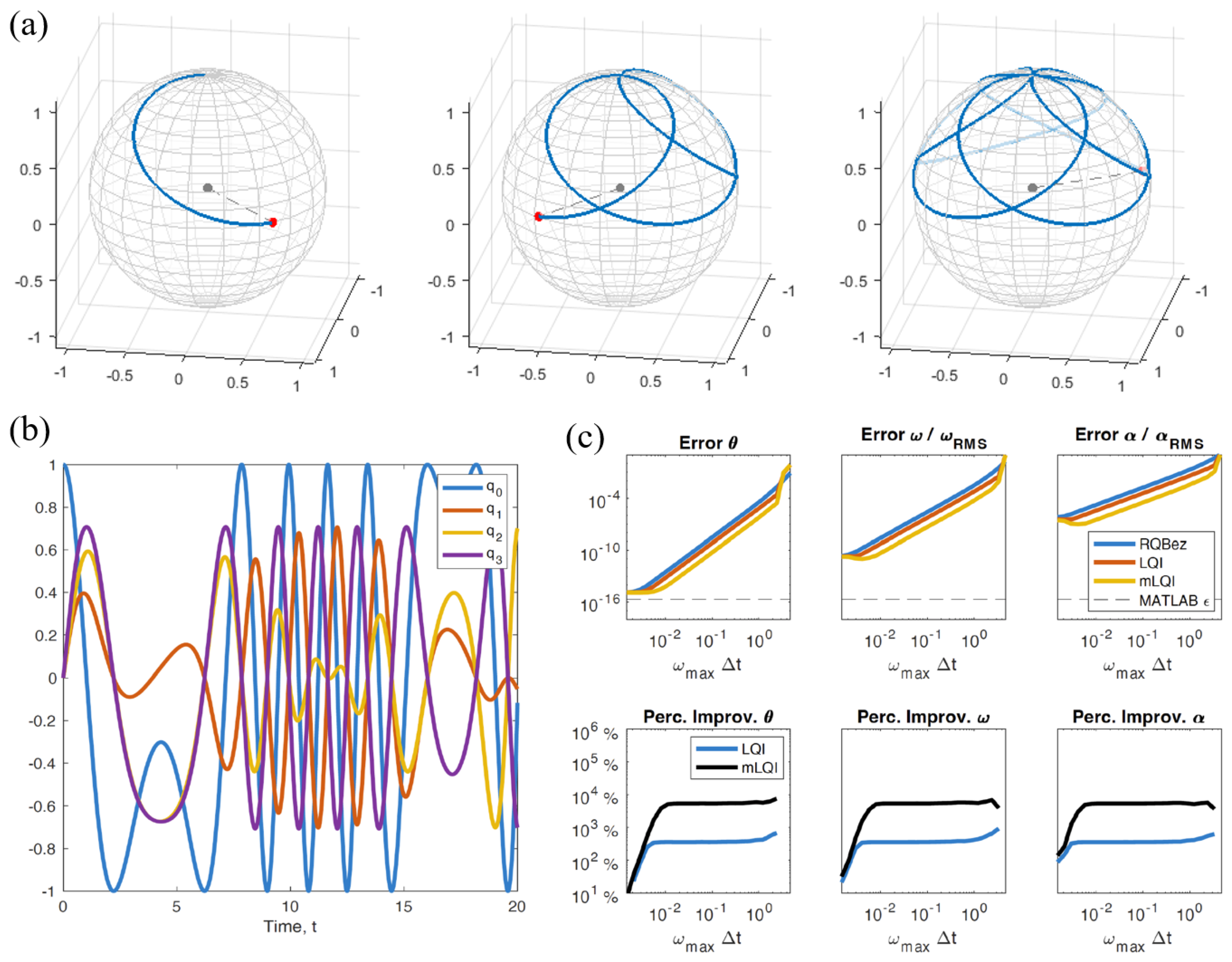
2.3. Example 3: Complex Mixed Rotation
2.4. Execution Time Comparison
3. Discussion and Conclusions
Author Contributions
Funding
Data Availability Statement
Acknowledgments
Conflicts of Interest
Abbreviations
| SLERP | Spherical Linear interpolation |
| SQUAD | Spherical and Quadrangle interpolation |
| RQBez | Renormalized Quaternion Bezier interpolation |
| LQI | Logarithmic Quaternion Interpolation |
| mLQI | modified Logarithmic Quaternion Interpolation |
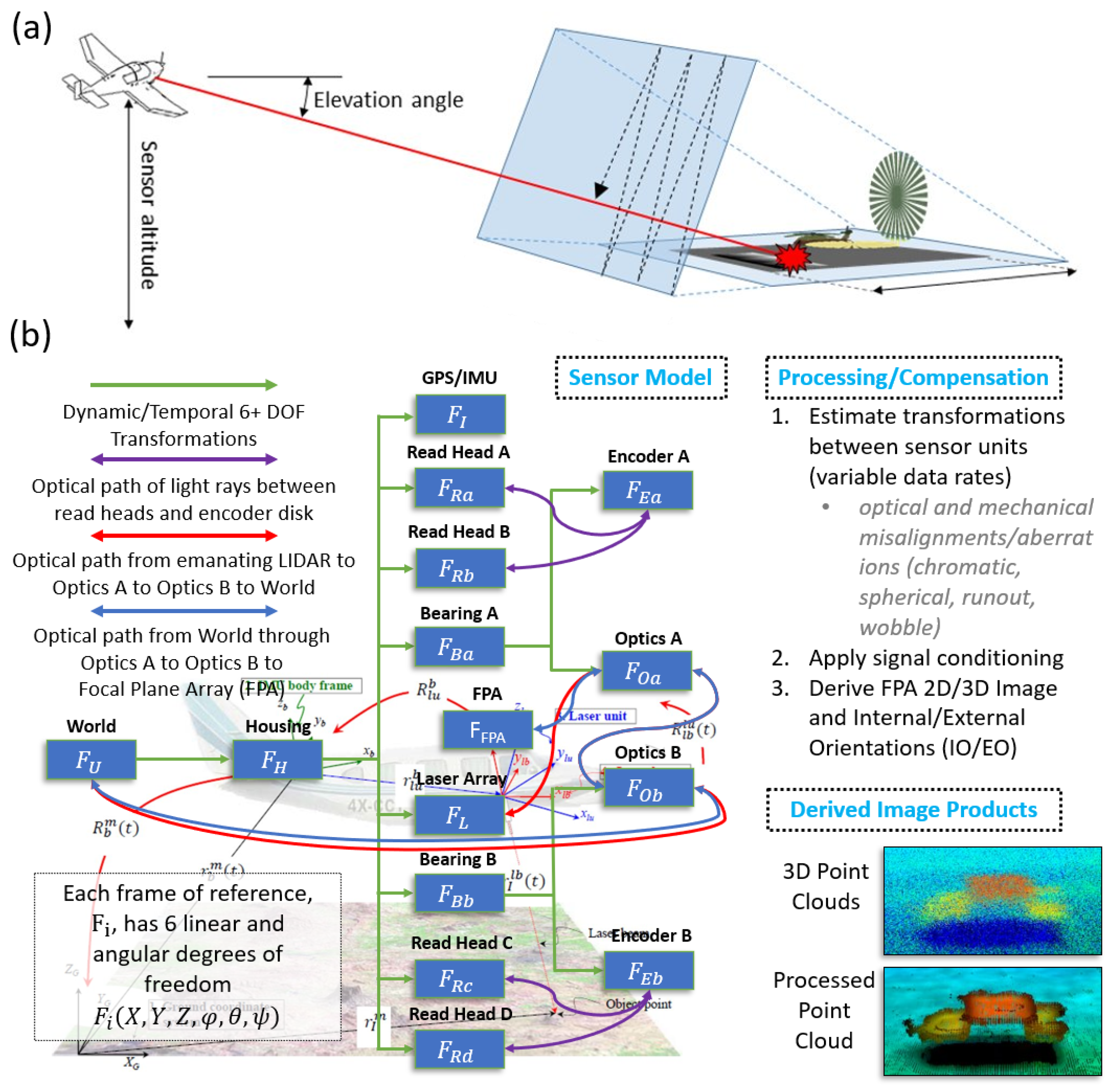
| KLMF | Kinematically Linked Model Framework |
| IMU | Inertial Measurement Unit |
| LIDAR | Light Detection and Ranging |
| GPS | Global Positioning System |
Appendix A. Derivative Equations
Appendix A.1. RQBez
Appendix A.2. LQI
Appendix A.3. mLQI
References
- Beange, K.H.; Chan, A.D.; Graham, R.B. Evaluation of wearable IMU performance for orientation estimation and motion tracking. In Proceedings of the 2018 IEEE International Symposium on Medical Measurements and Applications (MeMeA), Rome, Italy, 11–13 June 2018; pp. 1–6. [Google Scholar]
- Blanke, M.; Larsen, M.B. Satellite dynamics and control in a quaternion formulation. Technical University of Denmark, Department of Electrical Engineering. Tech. Rep. 2010. Available online: https://www.researchgate.net/profile/Mogens-Blanke/post/How-can-I-introduce-faults-to-Reaction-Wheel-unit/attachment/59d61fe479197b807797e581/AS%3A287324580663296%401445514926471/download/Satdyn_mb_2010f.pdf (accessed on 29 December 2022).
- Himberg, H.; Motai, Y. Head orientation prediction: Delta quaternions versus quaternions. IEEE Trans. Syst. Man Cybern. Part B (Cybern.) 2009, 39, 1382–1392. [Google Scholar] [CrossRef] [PubMed]
- Ober, D.B. Impact of rigorous modeling for a Geiger-mode light detection and ranging system on identifying uncalibrated component error sources and total propagated uncertainty. In Proceedings of the Laser Radar Technology and Applications XXVIII, SPIE, Orlando, FL USA, 3–4 May 2023. [Google Scholar]
- Ullrich, A.; Pfennigbauer, M. Linear LIDAR versus Geiger-mode LIDAR: Impact on data properties and data quality. In Proceedings of the Laser Radar Technology and Applications XXI. SPIE, Baltimore, MD, USA, 19–20 April 2016; Volume 9832, pp. 29–45. [Google Scholar]
- Ranacher, P.; Brunauer, R.; Van der Spek, S.; Reich, S. What is an appropriate temporal sampling rate to record floating car data with a GPS? ISPRS Int. J. Geo-Inf. 2016, 5, 1. [Google Scholar] [CrossRef]
- Young, A.D.; Ling, M.J.; Arvind, D.K. IMUSim: A simulation environment for inertial sensing algorithm design and evaluation. In Proceedings of the 10th ACM/IEEE International Conference on Information Processing in Sensor Networks, Chicago, IL, USA, 12–14 April 2011; pp. 199–210. [Google Scholar]
- Alaimo, A.; Artale, V.; Milazzo, C.; Ricciardello, A. Comparison between Euler and quaternion parametrization in UAV dynamics. In Proceedings of the AIP Conference Proceedings. American Institute of Physics, Antalya, Turkey, 24–28 April 2013; Volume 1558, pp. 1228–1231. [Google Scholar]
- Dam, E.B.; Koch, M.; Lillholm, M. Quaternions, Interpolation and Animation; Citeseer: University Park, PA, USA, 1998; Volume 2. [Google Scholar]
- Shoemake, K. Animating rotation with quaternion curves. In Proceedings of the 12th Annual Conference on Computer Graphics and Interactive Techniques, San Francisco, CA, USA, 22–26 July 1985; pp. 245–254. [Google Scholar]
- Shoemake, K. Quaternion Calculus and Fast Animation, Computer Animation: 3-D Motion Specification and Control; Siggraph: Los Angeles, CA, USA, 1987. [Google Scholar]
- Haarbach, A.; Birdal, T.; Ilic, S. Survey of higher order rigid body motion interpolation methods for keyframe animation and continuous-time trajectory estimation. In Proceedings of the 2018 International Conference on 3D Vision (3DV), Verona, Italy, 5–8 September 2018; pp. 381–389. [Google Scholar]
- Pu, Y.; Shi, Y.; Lin, X.; Hu, Y.; Li, Z. C2-Continuous Orientation Planning for Robot End-Effector with B-Spline Curve Based on Logarithmic Quaternion. Math. Probl. Eng. 2020, 2020, 2543824. [Google Scholar] [CrossRef]
- MATLAB. Version R2022a; The MathWorks Inc.: Natick, MA, USA, 2022. [Google Scholar]


Disclaimer/Publisher’s Note: The statements, opinions and data contained in all publications are solely those of the individual author(s) and contributor(s) and not of MDPI and/or the editor(s). MDPI and/or the editor(s) disclaim responsibility for any injury to people or property resulting from any ideas, methods, instructions or products referred to in the content. |
© 2023 by the authors. Licensee MDPI, Basel, Switzerland. This article is an open access article distributed under the terms and conditions of the Creative Commons Attribution (CC BY) license (https://creativecommons.org/licenses/by/4.0/).
Share and Cite
Parker, J.; Ibarra, D.; Ober, D. Logarithm-Based Methods for Interpolating Quaternion Time Series. Mathematics 2023, 11, 1131. https://doi.org/10.3390/math11051131
Parker J, Ibarra D, Ober D. Logarithm-Based Methods for Interpolating Quaternion Time Series. Mathematics. 2023; 11(5):1131. https://doi.org/10.3390/math11051131
Chicago/Turabian StyleParker, Joshua, Dionne Ibarra, and David Ober. 2023. "Logarithm-Based Methods for Interpolating Quaternion Time Series" Mathematics 11, no. 5: 1131. https://doi.org/10.3390/math11051131
APA StyleParker, J., Ibarra, D., & Ober, D. (2023). Logarithm-Based Methods for Interpolating Quaternion Time Series. Mathematics, 11(5), 1131. https://doi.org/10.3390/math11051131