Abstract
The observer design and dynamic output feedback control for a class of nonlinear networked systems are studied in this paper. The model of the networked systems is established by using T-S fuzzy method, and the state observer of the systems is designed when the states of the systems are unknown. On this basis, the sufficient conditions for the exponential stability of the system are explored by using the linear matrix inequality (LMI) method and Lyapunov stability theory. Then, the dynamic output feedback control of the systems is designed by using the observer states, which ensures that the states of the closed-loop systems and the error systems exponentially converge to the origin at the same time. Finally, a simulation example is given to illustrate the feasibility and effectiveness of the design method.
MSC:
93D15; 93D23
1. Introduction
With the progress of science and technology, especially the development of internet technology, the traditional point-to-point systems have been difficult to apply to the actual network engineering. The combination of network and control technology is an important development direction in the field of control in recent years, so network-based control came into being [1,2]. The closed-loop systems formed through the network is called networked control systems. Information is transmitted between sensors, controllers, actuators and other components through the network. Due to the introduction of network, the connection of the systems becomes convenient and easy, the systems performance is relatively stable, and the systems maintenance cost is relatively low. Due to the many advantages of networked systems, a large number of research reports on networked systems analysis and synthesis have emerged in recent years [3,4].
However, due to the characteristics of the network itself, the network induced delay is inevitable in the networked control systems. Network induced delay often occurs in the transmission of information between physical elements. As we all know, network induced delay often makes the systems performance worse or even unstable [5,6,7]. The stability and stabilization of networked systems with induced delays and data dropout were studied in [8]. A new extended Lyapunov functional was introduced, and a new freedom weight matrix was used to increase some degrees of freedom under the condition of sufficient stabilization. Merid et al. considered the packet dropout and scheduling problems of networked control systems [9]. Through the application of protocol and controller collaborative design method, the adverse effects of packet dropout and scheduling were solved. This method made use of the model predictive control framework and the flexible networked control systems architecture that allows distributed computing. The H∞ control problem for a class of linear time-varying networked systems was studied in [10]. An observer based controller was designed to ensure the performance of the H∞ performance of the closed-loop systems in a given finite time. The sufficient conditions for the existence of the desired controller were established by using stochastic analysis and complete square method. The problem of static output feedback control for networked systems with quantization and Markov packet dropout was studied in [11]. A new quantization structure was proposed to model the closed-loop systems as a Markov jump linear systems with partially unknown transition probabilities. The design method of static output feedback controller was given to ensure the stability of the closed-loop systems corresponding to the proposed quantization structure. Domagoj et al. employed the hybrid-systems-with-memory formalism to attain transmission intervals and delays that provably stabilized networked systems [12]. Nonlinear time-varying plants and controllers with variable discrete and distributed input, output and state delays along with non-constant discrete and distributed network delays were considered. The stability and controller design of networked systems with network induced delay and stochastic sampling interval were studied in [13]. By introducing a new matrix decomposition method, a stabilizing controller was designed to make the closed-loop systems stochastic stable.
Fuzzy control is an effective way to solve the control problem of nonlinear systems. In particular, T-S fuzzy control method is used to approximate the mathematical model of nonlinear systems to linear related large-scale systems, which can effectively reduce the difficulty of systems analysis and design [14,15,16]. The exponential stability analysis and controller synthesis of positive T-S fuzzy discrete systems with time-varying delays were discussed in [17]. By constructing a new Lyapunov functional, the exponential stability condition and controller design strategy of fuzzy systems were obtained. The stability of control systems based on fuzzy model of sampled data was studied in [18]. T-S fuzzy model was used to represent continuous time nonlinear objects. A design method of sampled data fuzzy controller was proposed. The stability and stabilization of T-S fuzzy systems with time-varying delays were studied in [19]. By constructing an appropriate Lyapunov functional and using the method of cross convex inequality, the less conservative stability criteria and stability conditions were obtained. In order to exploit the advantages of data-driven control and fuzzy control, Roman et al. proposed the virtual reference feedback tuning of a combination of two control algorithms, active disturbance rejection control as a representative data-driven control algorithm and fuzzy control in [20]. The main benefit of this combination was the automatic optimal tuning in a model-free manner of the parameters of the combination of active disturbance rejection control with proportional-derivative T-S fuzzy control.
The above results are all about the research results of linear networked systems. The research on nonlinear networked systems is a challenging and meaningful topic. At present, some results have been obtained in the research of nonlinear networked systems [21,22,23,24,25,26]. The robust control problem of a class of T-S fuzzy networked systems with stochastic sensor faults was studied in [27]. Based on Lyapunov stability theory and stochastic analysis technology, the stability conditions and the controller design strategy were obtained. An improved cone complementary linearization algorithm was introduced to solve the nonlinear matrix inequalities in the controller design. A robust H∞ fault detection filter was designed for a class of discrete-time nonlinear networked control systems in [28]. The fault detection filter is designed by using T-S fuzzy model, and the sufficient conditions for the existence of the expected filter were given. Bouazza proposed state feedback control for a class of nonlinear networked control systems with system delay and packet loss [29]. The stability of this kind of systems was realized by dynamic output feedback. The sufficient conditions were given to ensure the state variables and state estimation errors converge to the origin. Yoneyama et al. studied the stabilization of nonlinear networked systems described by T-S fuzzy systems [30]. The generalized controller made the networked control systems asymptotic stable. The stabilization problem of a class of T-S fuzzy networked systems was studied in [31]. The member level of the object model was incorporated into the controller synthesis criterion to increase the maximum allowable delay in the closed-loop systems. The applicability and superiority of the proposed scheme compared with the existing methods were verified by some examples. Barmak et al. studied the fault detection problem of nonlinear networked systems subject to both communication constraints and packet dropouts [32]. T-S fuzzy model was employed to describe the nonlinear networked systems. Based on the theory of optimal periodic residual generator, an observer was proposed to solve the problem of fault detection of nonlinear networked systems. Magdi et al. studies the state feedback control problem for a class of nonlinear networked systems with norm-bounded uncertainties [33]. The state feedback stability conditions that ensure robust asymptotic stability and strict dissipative stability were given, and a new LMI criterion for strict dissipative stability analysis and feedback synthesis was established. Lian et al. studied the security control problem for nonlinear networked control systems under cyber attacks [34]. The networked control systems contained parameter uncertainties, time delays, and cyber attacks. A control method based on hybrid trigger is established to ensure the robust stability of the closed-loop systems. Cai et al. studied the dissipative analysis issue of T-S fuzzy networked control system with stochastic cyber-attacks and voluntary defense strategy [35]. A novel time-delay-product relaxed condition was proposed, which fully excavates the time-varying delay information under the given conditions. By using reciprocally convex matrix inequality, proper integral inequalities, and the linear convex combination method, a novel criterion and the corresponding control algorithm were developed. Zheng et al. discussed the exponentially mean-square stability of stochastic T-S fuzzy networked systems [36]. By designing fuzzy-basis-dependent Lyapunov functional, the delay-dependent stability conditions were obtained, and it was proved that the closed-loop systems was exponentially mean square stable. Prakash et al. studied the H∞ control scheme of distributed delay T-S fuzzy networked control systems [37]. The candidate Lyapunov function related to fuzzy membership was designed. The switching concept related to the change rate of membership function was introduced to design the optimal control gain matrix for the considered system.
However, the above results mainly focus on the asymptotic stability of the networked systems, while the research on the exponential stability and dynamic output feedback control is rare. For this reason, based on the previous studies, the sufficient conditions of exponential stability and dynamic output feedback control for a class of nonlinear networked systems will be explored in this paper by using T-S fuzzy method and linear matrix inequality.
2. Preliminaries
Consider the following typical fuzzy networked systems with communication delay shown in Figure 1.
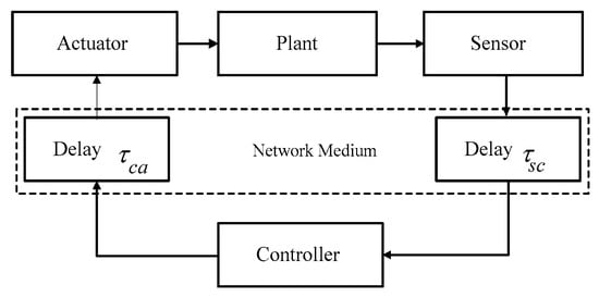
Figure 1.
A typical networked control systems.
Rule :
IF is and is , …, and is
THEN
where is the premise variable, is the systems state, is the number of IF-THEN rules, are fuzzy sets, is the control input, is the systems output, are constant matrices, are input matrix, are output matrix.
In Figure 1, and are the sensor-controller and controller-actuator delay respectively. Then the communication delay is given by . Using single point fuzzification, product inference engine and central fuzzy elimination method, the global fuzzy model of systems (1) can be described as
where is the initial condition of the state,
where is the membership degree of corresponding to , satisfying
And we definite
The following fuzzy observer based on T-S model for systems (2) will be designed
where are constant matrices.
And then, a fuzzy controller based on the above observer will be designed
The observer error is defined as
The closed-loop systems can be obtained from Equations (2)–(5)
With (3), (5) and (6), the error systems can be obtained
where .
The purpose of this paper is to design a fuzzy controller (4) so that the closed-loop systems and the error systems exponentially stable.
Remark 1.
The fuzzy networked systems is modeled by using T-S fuzzy approach. The fuzzy observer is designed by using the output of the systems (2). In the process of establishing the systems model, we regard the delay from sensor to controller and control to actuator as the control input delay, which can facilitate the controller design. Although it will increase the limitation of the systems in practical application, it will not affect the application of this modeling method in non remote networked systems, such as networked industrial robot systems, industrial transmission system, etc.
3. Main Results
Definition 1
([7]). For the systems (2), if there exist constants and such that
the systems (2) is exponentially stable.
Lemma 1
([8]). The linear matrix inequality
is equivalent to
where the matrices depend on .
3.1. Design of Fuzzy Observer
Theorem 1.
For the given constantsand, if there exist matricesand positive-definite matricessuch that the following matrix inequality holds
the error systems (7) is exponentially stable.
Proof.
The Lyapunov function is selected as
where is a constant to be determined, is a positive-definite matrix.
Following the state trajectory of the systems (7), we obtain
It can be seen from reference [6]
therefore
When the matrix inequality (8) holds, it can be obtained by substituting it into the above equality
Then
It is easy to know from the expression of ,
Combing (9) and (10), we obtain
with Defintion 1, we know that the error systems (7) is exponentially stable. □
Remark 2.
Theorem 1 gives a sufficient condition (8) for exponential stability of the error systems. And, the exponential stability degreecan be obtained by solving the condition (8).
3.2. Design of Fuzzy Controller
Theorem 2.
For the given constantsand, if there exist a constant, matricesand positive-definite matrices, such that the following matrix inequalities hold
where
with the controller, the closed-loop systems (6) and the error systems (7) are exponentially stable.
Proof.
The Lyapunov function is selected as
where is a constant to be determined, are positive-definite matrices.
Following the state trajectory of the systems (6), we obtain
where is a constant, and
If the matrix inequality (12) holds, the above equality can be changed as
When , we have
According to Theorem 1, when the matrix inequality (11) holds, the error systems (7) is exponentially stable, that is, the error is exponentially stable, and the state of the closed-loop systems is also exponentially stable according to the Equation (14), so that the closed-loop systems (6) and the error systems (7) are exponentially stable.
When , the inequality (13) can be changed as
therefore
It is easy to know from the expression of
Combing (15) and (16), we obtain
the closed-loop systems (6) is exponentially stable. It is also known from Theorem 1 that when the matrix inequality (11) holds, the error systems (7) is exponentially stable, so that the closed-loop systems (6) and the error systems (7) are exponentially stable.
In a word, when the matrix inequalities (11) and (12) hold, the closed-loop systems (6) and the error systems (7) are exponentially stable. □
Remark 3.
In Theorem 2, the sufficient conditions (11)–(12) are not linear matrix inequalities, which cannot be solved by the LMI toolbox in MATLAB.
Theorem 3.
For the given constants
and , if there exist constant , matrices and positive-definite matrices such that the following matrix inequalities hold
with the controller , the closed-loop systems (6) and the error systems (7) are exponentially stable.
Proof.
Letting , the matrix inequality (11) can be changed as the inequality (17). Multiplying the matrix on both sides of the matrix inequality (12), and let , we can obtain
Letting , and with Lemma 1, the above inequality is equivalent to the inequality (18). □
Remark 4.
With Lemma 1, the sufficient conditions (17)–(18) are obtained in terms of linear matrix inequality in Theorem 3. The exponential stability and of the closed-loop systems and the error systems can be solved by the LMI toolbox in MATLAB, and the maximum values ofcan be optimized.
Remark 5.
In Theorem 3, when the values of the constantsare given, the conditions (17)–(18) are linear matrix inequalities. If we want to optimize the exponential stability degree, we can select different values of, and solve the condition (17)–(18) repeatedly, so as to get the optimization results.
4. Maximum Delay Bound Estimation
Theorem 3 gives the sufficient condition (17)–(18) on the output feedback controller. When the values of the constants are given, the conditions (17)–(18) are linear matrix inequalities. Consequently, the original non-convex problem can be transformed into the following minimization problem involving LMI condition, which is solved by Cone Complementarity Linearization Method (CCLM).
With given in the Theorem 2, the inequalities (11)–(12) are established when is in a certain range. Then is assumed as the maximum value which is able to achieve, and the following set of optimization matrix inequalities is used to obtain as
The optimization problem (19) is solved via Cone Complementarity Linearization Method (CCLM), since the LMI toolbox is unable to be employed to solve the set of nonlinear matrix inequalities (19) directly. Then inequalities (11) and (12) are converted into (17) and (18). The convex optimization problem (19) is split into the following linear optimization problem with three steps.
Step 1. Select a sufficiently small initial such that the following matrix inequalities have feasible solution
Set
Step 2. With given from step 1, find feasible constant of and feasible matrices of satisfying the inequalities (20). Set .
Step 3. For variables , solve the following convex optimization problem
Set
There exist two cases for the results of this step and it is described as follows:
Case 1. There exist feasible solutions of (21). That is, it gets a reasonable value for . Make an update on , increase by a small amount, and then return to step 2.
Case 2. There are not feasible solutions of (21). Make , and then return to step 3. When an iteration index is beyond a pre-limit value, the algorithm is ended, and the maximum value of is obtained.
5. Simulation
Consider the following networked systems such as (2)
where
By using the algorithm in [26], the state feedback controller can be obtained as
On the other, by using the proposed approach in this paper to solve the linear matrix inequality (17)–(18), we obtain
The dynamic output feedback controller can be obtained as
By selecting the initial value condition such as
the sampling time , the response curves of the systems state are as Figure 2, Figure 3 and Figure 4.
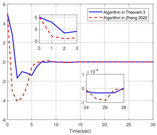
Figure 2.
The response curves of the systems state . Red dotted line is under algorithm in [26].
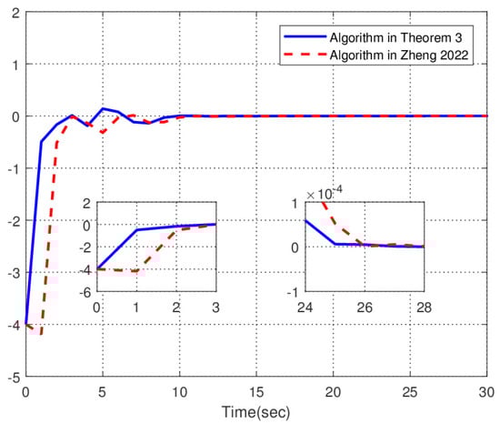
Figure 3.
The response curves of the systems state . Red dotted line is under algorithm in [26].
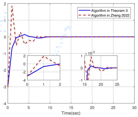
Figure 4.
The response curves of the systems state . Red dotted line is under algorithm in [26].
Figure 2 shows the control effect of systems state under the two different algorithms. The solid line is the response curve of the systems state under the action of the fuzzy controller designed in Theorem 3. The dotted line is the response curve of the systems state under the action of state feedback control in [26]. The solid line converges to a small neighborhood of origin in just 7 s. Although the curve is not smooth enough, the overshoot is small and the amplitude does not exceed 2. The dotted line converges to a small neighborhood of origin in 9 s, and the convergence speed is slightly slow. Although the curve is smooth, the overshoot is large, and the amplitude reaches 4.
Figure 3 shows the control effect of systems state under the two different algorithms. The solid line is the response curve of the systems state under the action of the fuzzy controller designed in Theorem 3. The dotted line is the response curve of the systems state under the action of state feedback control in [26]. Both the solid line and dotted line converge to a small neighborhood of origin in about 10 s, the overshoot of the solid line is small, and the amplitude does not exceed 0.2. The overshoot of the dotted line is large, and the amplitude is greater than 4.
Figure 4 shows the control effect of systems state under the two different algorithms. The solid line is the response curve of the systems state under the action of the fuzzy controller designed in Theorem 3. The dotted line is the response curve of the systems state under the action of state feedback control in [26]. The solid line converges to a small neighborhood of origin within 6 s. The curve is smooth enough, the overshoot is small, and the amplitude does not exceed 0.1. The dotted line converges to a small neighborhood of origin only after 10 s, and the convergence speed is slow. The smoothness of the curve is poor, the overshoot is large, and the amplitude reaches 1.8.
In order to further compare the advantages and disadvantages of the algorithm given in Theorem 3 and the algorithm in [26], the Integral Absolute Error (IAE) performance function
is introduced to simulate and analyze the systems, and the change curves of IAE performance index of the systems are obtained as Figure 5.
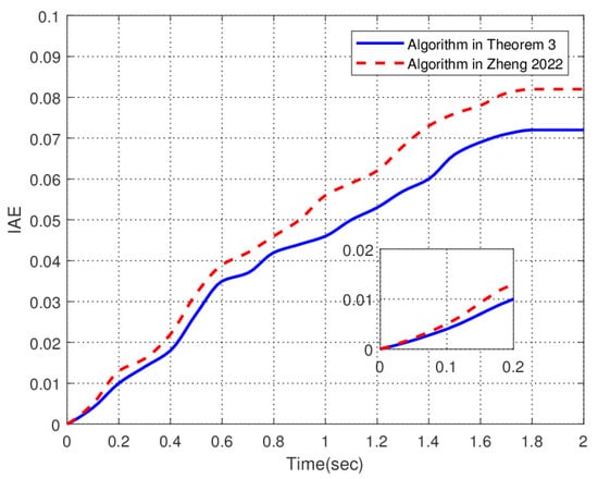
Figure 5.
The change curves of IAE performance index. Red dotted line is under algorithm in [26].
Figure 5 shows the changes of IAE performance index of the systems under the two different algorithms. The solid line is the change curve of IAE performance index under the action of the fuzzy controller designed in Theorem 3. The dotted line is the change curve of IAE performance index under the action of state feedback control in [26]. The dotted line reaches the peak value 0.082 in 1.7 s. The solid line reaches the peak value 0.072 in 1.8 s. On the whole, the gradient of the dotted line is larger than the solid line, and the rising speed is relatively fast.
In a word, the algorithm given in Theorem 3 is superior to [26] in convergence speed and smoothness.
6. Discussion
The contribution of this paper is to give an exponential stability method to deal with networked systems with communication delay. The innovation of this paper lies in the design of exponential stable state observer, and the design of dynamic output feedback control is given in the form of linear matrix inequality. The purpose of this paper is to provide an effective way to reduce the influence of network communication delay on the networked systems, improve systems performance, and solve practical problems in network engineering. In addition, it is worth mentioning that our results can be extended to other types of networked systems, such as distributed delay, fast varying delay, random delay, etc., which will be our next research work.
7. Conclusions
In this paper, the exponential stable state observer and dynamic output feedback control of fuzzy networked systems are designed. The main work are as follows: (I) considering the influence of network communication delay on the systems, a more practical mathematical model of networked systems is established by using T-S fuzzy method. (II) Combined with Lyapunov stability theory, the exponentially stable state observer is designed by using linear matrix inequality method. (III) By using the matrix inequality transformation technique, the nonlinear stability condition is equivalent to the form of linear matrix inequality, and the design method of exponential stability control of the systems is obtained at the same time. Because the obtained conditions can be easily solved by MATLAB, this method is easier to be applied to engineering practice. Unfortunately, the obtained sufficient conditions in Theorem 3 are delay-independent and less conservative. How to develop an output feedback control for T-S fuzzy networked systems with varying delay will be a topic for our future works. Applying the proposed method to stochastic networked control systems is another of our future topics.
Author Contributions
H.Y.: Conceptualization, methodology, software, investigation, writing-original draft, validation. F.G.: software, resources, writing-review and editing, supervision. All authors have read and agreed to the published version of the manuscript.
Funding
This work was partially supported by the National Natural Science Foundation of China under Grant 61073065, the Young Teacher Training Plan of Colleges and Universities of Henan Province under Grant 2019GGJS192, the Education Department of Henan Province Key Foundation under Grant 23B110001.
Institutional Review Board Statement
The study was conducted according to the guidelines of the Declaration of Helsinki and approved by the Institutional Review Board.
Informed Consent Statement
Not applicable.
Data Availability Statement
Not data were used to support this study.
Conflicts of Interest
The authors declare no conflict of interest.
References
- Kundu, A.; Quevedo, D.E. Stabilizing scheduling policies for networked control systems. IEEE Trans. Control. Netw. Syst. 2020, 7, 163–175. [Google Scholar] [CrossRef]
- Wang, Y.L.; Yu, S.H. An improved dynamic quantization scheme for uncertain linear networked control systems. Automatica 2018, 92, 244–248. [Google Scholar] [CrossRef]
- Liu, L.; Liu, X. Delayed observer-based H∞ control for networked control systems. Neurocomputing 2016, 179, 101–109. [Google Scholar] [CrossRef]
- Li, Y.J.; Liu, G.P.; Sun, S.L.; Tan, C. Prediction-based approach to finite-time stabilization of networked control systems with time delays and data packet dropouts. Neurocomputing 2019, 329, 320–328. [Google Scholar] [CrossRef]
- Selivanov, A.; Fridman, E. Observer-based on input-to-state stabilization of networked control systems with large uncertain delays. Automatica 2016, 74, 63–70. [Google Scholar] [CrossRef]
- Chen, G.; Xia, J.; Zhuang, G. Improved delay-dependent stabilization for a class of networked control systems with nonlinear perturbations and two delay components. Appl. Math. Comput. 2018, 316, 1–17. [Google Scholar] [CrossRef]
- Hua, C.C.; Yu, S.C.; Guan, X.P. Finite-time control for a class of networked control systems with short time-varying delays and sampling jitter. Int. J. Autom. Comput. 2015, 12, 448–454. [Google Scholar] [CrossRef]
- Arash, F.; Reza, M.E. Improved stabilization method for networked control systems with variable transmission delays and packet dropout. ISA Trans. 2014, 53, 1746–1753. [Google Scholar]
- Merid, L.; Dragan, N.; Daniel, E. Robust stability of a class of networked control systems. Automatica 2016, 73, 117–124. [Google Scholar]
- Zou, L.; Wang, Z.D.; Gao, H.J. Observer-based H∞ control of networked systems with stochastic communication protocol: The finite-horizon case. Automatica 2016, 63, 366–373. [Google Scholar] [CrossRef]
- Song, J.S.; Chang, X.H. H∞ controller design of networked control systems with a new quantization structure. Appl. Math. Comput. 2020, 376, 125070. [Google Scholar] [CrossRef]
- Domagoj, T. Stabilizing transmission intervals and delays in nonlinear networked control systems through hybrid-system- with-memory modeling and Lyapunov-Krasovskii arguments. Nonlinear Anal. Hybrid Syst. 2020, 36, 100834. [Google Scholar]
- Sun, H.Y.; Sun, J.; Chen, J. Analysis and synthesis of networked control systems with random network-induced delays and sampling intervals. Automatica 2021, 125, 109385. [Google Scholar] [CrossRef]
- Ma, Y.; Chen, M.; Zhang, Q. Non-fragile static output feedback control for singular T-S fuzzy delay-dependent systems subject to Markovian jump and actuator saturation. J. Frankl. Inst. 2016, 353, 2373–2397. [Google Scholar] [CrossRef]
- Qi, W.H.; Park, J.H.; Cheng, J.; Chen, X.M. Stochastic stability and L1 -gain analysis for positive nonlinear semi-Markov jump systems with time-varying delay via T-S fuzzy model approach. Fuzzy Sets Syst. 2019, 371, 110–122. [Google Scholar] [CrossRef]
- Chi, R.; Li, H.; Shen, D.; Hou, Z.; Huang, B. Enhanced P-type control: Indirect adaptive learning from set-point updates. IEEE Trans. Autom. Control. 2022. [Google Scholar] [CrossRef]
- Meng, M.; Lam, J.; Feng, J.; Zhao, X.D.; Chen, X.M. Exponential stability analysis and H∞ synthesis of positive T-S fuzzy systems with time-varying delays. Nonlinear Anal. Hybrid Syst. 2017, 24, 186–197. [Google Scholar] [CrossRef]
- Wang, L.K.; Lam, H.K. New stability criterion for continuous-time Takagi-sugeno fuzzy systems with time varying delay. IEEE Trans. Cybern. 2019, 49, 1551–1556. [Google Scholar] [CrossRef]
- Yin, Z.; Jiang, X.; Tang, L. On stability and stabilization of T-S fuzzy systems with multiple random variables dependent time-varying delay. Neurocomputing 2020, 412, 91–100. [Google Scholar] [CrossRef]
- Roman, R.C.; Precup, R.E.; Petriu, E.M. Hybrid data-driven fuzzy active disturbance rejection control for tower crane systems. Eur. J. Control. 2021, 58, 373–387. [Google Scholar] [CrossRef]
- Oliveiva, T.; Palhares, R. Improved Takagi-sugeno fuzzy output tracking control for nonlinear networked control systems. J. Frankl. Inst. 2017, 354, 7280–7305. [Google Scholar] [CrossRef]
- Ahmad, S.; Ahmad, M.E.; Mohammad, E.; Mohammed, S. Improving the performance of networked control systems with time delay and data dropouts based on fuzzy model predictive control. J. Frankl. Inst. 2018, 355, 7201–7225. [Google Scholar]
- Li, Y.H.; Qi, J.; Liang, Y. Quantized L1 filtering for stochastic networked control systems based on T-S fuzzy model. Signal Process. 2020, 167, 107249. [Google Scholar] [CrossRef]
- Li, X.H.; Ye, D. Observer-based defense control for networked Takagi-sugeno fuzzy systems against asynchronous DoS attacks. J. Frankl. Inst. 2021, 358, 6136–6160. [Google Scholar] [CrossRef]
- Xu, S.D.; Wen, H.; Wang, X.Y. Observer-based robust fuzzy control of nonlinear networked systems with actuator saturation. ISA Trans. 2022, 123, 122–135. [Google Scholar] [CrossRef]
- Zheng, W.; Zhang, Z.M.; Sun, F.C.; Wen, S.H. Robust stability analysis and feedback control for networked control systems with additive uncertainties and signal communication delay via matrices transformation information method. Inf. Sci. 2022, 582, 258–286. [Google Scholar] [CrossRef]
- Peng, C.; Fei, M.R.; Tian, E. Networked control for a class of T-S fuzzy systems with stochastic sensor faults. Fuzzy Sets Syst. 2013, 212, 62–77. [Google Scholar] [CrossRef]
- Ding, W.G.; Mao, Z.H.; Jiang, B.; Shi, P.; He, X. H∞ fault detection for a class of T-S fuzzy model-based nonlinear networked control systems. IFAC Proc. Vol. 2014, 47, 11647–11652. [Google Scholar] [CrossRef]
- Bouazza, K. Dynamic output feedback for nonlinear networked control system with system delays and packet dropout. IFAC Proc. Vol. 2014, 47, 6496–6501. [Google Scholar] [CrossRef]
- Yoneyama, J.; Kenta, H. Stability analysis and synthesis for nonlinear networked control systems. IFAC-Pap. 2016, 49, 297–302. [Google Scholar] [CrossRef]
- Sepideh, M.; Reza, M.E.; Ahmad, A.; Mohsen, B. T-S fuzzy controller design for stabilization of nonlinear networked control systems. Eng. Appl. Artif. Intell. 2016, 50, 35–141. [Google Scholar]
- Barmak, B.; Behrooz, R.; Zahra, R. Fuzzy-model-based fault detection for nonlinear networked control systems with periodic access constraints and Bernoulli packet dropouts. Appl. Soft Comput. 2019, 80, 465–474. [Google Scholar]
- Mahmoud, M.S.; Xia, Y.Q.; Zhang, S.X. Robust packet-based nonlinear fuzzy networked control systems. J. Frankl. Inst. 2019, 356, 1502–1521. [Google Scholar] [CrossRef]
- Lian, Z.; Shi, P.; Lim, C.C. Hybrid-triggered interval type-2 fuzzy control for networked systems under attacks. Inf. Sci. 2021, 567, 332–347. [Google Scholar] [CrossRef]
- Cai, X.; Shi, K.B.; She, K.; Zhong, S.M.; Kwon, O.; Tang, Y.Q. Voluntary defense strategy and quantized sample-data control for T-S fuzzy networked control systems with stochastic cyber-attacks and its application. Appl. Math. Comput. 2022, 423, 126975. [Google Scholar] [CrossRef]
- Zheng, W.; Zhang, Z.M.; Lam, H.K.; Sun, F.C.; Wen, S.H. LMIs-based stability analysis and fuzzy-logic controller design for networked systems with sector nonlinearities: Application in tunnel diode circuit. Expert Syst. Appl. 2022, 198, 116627. [Google Scholar] [CrossRef]
- Mani, P.; Joo, Y.H. Fuzzy-logic-based event-triggered H∞ control for networked systems and its application to wind turbine systems. Inf. Sci. 2022, 585, 144–161. [Google Scholar] [CrossRef]
Disclaimer/Publisher’s Note: The statements, opinions and data contained in all publications are solely those of the individual author(s) and contributor(s) and not of MDPI and/or the editor(s). MDPI and/or the editor(s) disclaim responsibility for any injury to people or property resulting from any ideas, methods, instructions or products referred to in the content. |
© 2022 by the authors. Licensee MDPI, Basel, Switzerland. This article is an open access article distributed under the terms and conditions of the Creative Commons Attribution (CC BY) license (https://creativecommons.org/licenses/by/4.0/).