
Classical and Bayesian Inference of a Progressive-Stress Model for the Nadarajah–Haghighi Distribution with Type II Progressive Censoring and Different Loss Functions


Abstract
:1. Introduction
2. A Cumulative Exposure Model of NH Distribution
- -
- Under usual conditions, the lifetime of a unit follows NH().
- -
- The progressive-stress (t) is directly proportional to the time t with constant rate , i.e., .
- -
- The scale parameter of the CDF in (2) satisfies the inverse power law, as follows
- -
- It is assumed that a and b are unknown physical positive parameters and need to be estimated.
- -
- Assume n is the total number of units tested, are the stress levels in the test, and is the use stress. Under each progressive-stress level, identical units are tested, and the progressive type II censoring is performed as follows: When the first failure occurs, units are picked at random from the remaining surviving units. When the second failure occurs, items from the remaining units are withdrawn at random. When the failure occurs, , the test is terminated, and all remaining items are removed.
- -
- The complete samples and type II censored samples are clearly specific examples of this technique. Under the progressive-stress , the observed progressive-censoring data are < , .
- -
- The linear cumulative exposure model (CEM) accounts for the effect of changing stress; for more details, see [13].
- -
- The CDF in progressive stress, , and the linear cumulative exposure model is given as followswhere , F (·) denotes the CDF of the NH distribution under progressive-stress with scale parameter λ. Thus,The corresponding PDF is given bywhere
3. Maximum Likelihood Estimation
4. Bayesian Estimation
Bayes Estimation Using BSEL and BLINEX Loss Functions
- Step 1:
- For the parameters (, ), set the initial guess to (, ).
- Step 2:
- Set j = 1.
- Step 3:
- Create and where is the variance–covariance matrix.
- Step 4:
- Compute .
- Step 5:
- With probability accept (, ),
- Step 6:
- To obtain B number of samples for the parameters (, ), repeat steps (3) to (5) B times.
5. Interval Estimation
5.1. Asymptotic Confidence Interval
5.2. HPD Interval of Credibility
5.3. Bootstrap Confidence Intervals
- (1)
- Calculate the MLE values of the parameters using the original data , and .
- (2)
- To make a bootstrap sample use the variables , and .
- (3)
- The bootstrap estimates , , and , respectively, are obtained based on .
- (4)
- To obtain the bootstrap samples, repeat steps 1–3 several times and organize each estimate in ascending orderThe percentile bootstrap CIs for are then calculated as follows:where and
6. Simulation Study
- Step 1:
- Using the algorithm presented in [10], progressively type II censored random samples are generated from the uniform (0,1) distribution , for given values of .
- Step 2:
- To compare the performance of the estimation procedures developed in the study, we consider the following two schemes for each stress:Scheme 1: , .Scheme 2: , .
- Step 3:
- Progressively type II censored random samples are produced, and from inverse CDF (3), we specify the values of parameters as follows:In Table 1 .In Table 2 , andIn Table 3 , and .In Table 4 ( and .In Table 5 (), , and .In Table 6 (, , and .
- Step 4:
- The MLEs are obtained numerically by solving the likelihood equations with respect to () in (8)–(10) by using an iterative Newton–Raphson algorithm using the maxlik function of the “maxlik” package in the R program; for more information in this topic see [30].
- Step 5:
- Based on (15)–(17), and the MH algorithm, the Bayesian estimations with the BSEL and BLINEX loss functions of the parameters () are computed by (13) and (14), respectively.
- Step 6:
- The above steps are repeated I times based on I different samples, and then the average of likelihood and Bayesian estimations are computed, with their MSE, bias, and length of confidence intervals (LCI) of the parameters ().
- Step 7:
- In length of CI (LCI) of the MLE of each parameter, we compute the ACI for likelihood estimators and bootstrap CIs with the percentile algorithm and t algorithm, which can be denoted as LBP and LBT, respectively. In the LCI of Bayesian estimation, we compute the HPD for each loss function, denoted by the LCCI.

| k = 2 | θ = 1.7, a = 1.3, b = 2 | MLE | BSEL | BLINEX (c = −0.5) | BLINEX (c = 0.5) | MLE | BSEL | BLINEX (c = −0.5) | BLINEX (c = 0.5) | ||||||||
|---|---|---|---|---|---|---|---|---|---|---|---|---|---|---|---|---|---|
| n1, n2 | Scheme | r | Bias | MSE | Bias | MSE | Bias | MSE | Bias | MSE | LCI | LBP | LBP | LCCI | LCCI | LCCI | |
| 20, 15 | 1 | 65% | θ | −0.6751 | 1.5008 | −0.1938 | 0.0886 | −0.1172 | 0.0801 | −0.2619 | 0.1099 | 4.0094 | 0.1331 | 0.1271 | 0.8592 | 0.9821 | 0.7748 |
| a | 0.3824 | 1.5335 | −0.0521 | 0.0788 | 0.0209 | 0.0994 | −0.1174 | 0.0740 | 4.6193 | 0.1432 | 0.1453 | 1.0048 | 1.1145 | 0.8922 | |||
| b | 0.0673 | 0.6760 | −0.2972 | 0.1145 | −0.2616 | 0.0964 | −0.3314 | 0.1345 | 3.2139 | 0.0998 | 0.0993 | 0.6315 | 0.6551 | 0.6181 | |||
| 85% | θ | −0.4879 | 0.7308 | −0.0879 | 0.0657 | −0.0097 | 0.0736 | −0.1581 | 0.0724 | 2.7529 | 0.0899 | 0.0894 | 0.9552 | 1.0524 | 0.8647 | ||
| a | 0.5008 | 0.9984 | 0.0504 | 0.0612 | 0.0195 | 0.0890 | 0.0426 | 0.0691 | 3.3911 | 0.1105 | 0.1101 | 0.9821 | 0.9834 | 0.9084 | |||
| b | 0.0625 | 0.6469 | −0.1622 | 0.0558 | −0.1260 | 0.0471 | −0.1967 | 0.0667 | 3.1026 | 0.0978 | 0.0965 | 0.6718 | 0.6934 | 0.6551 | |||
| 2 | 65% | θ | 0.0872 | 0.5633 | 0.0550 | 0.0583 | 0.1391 | 0.0909 | −0.0206 | 0.0450 | 2.9235 | 0.0894 | 0.0875 | 0.9262 | 1.0470 | 0.8281 | |
| a | −0.2725 | 0.5104 | 0.0517 | 0.1058 | 0.1262 | 0.1418 | −0.0158 | 0.0866 | 2.5902 | 0.0805 | 0.0818 | 1.2014 | 1.3056 | 1.0823 | |||
| b | 0.5035 | 0.8594 | 0.0607 | 0.0411 | 0.1011 | 0.0500 | 0.0218 | 0.0360 | 3.0529 | 0.0908 | 0.0915 | 0.7305 | 0.7490 | 0.7048 | |||
| 85% | θ | 0.0823 | 0.5078 | 0.0542 | 0.0580 | 0.1346 | 0.0879 | −0.0171 | 0.0448 | 2.8345 | 0.0804 | 0.0803 | 0.9137 | 0.9103 | 0.8448 | ||
| a | −0.1801 | 0.4902 | 0.0863 | 0.1041 | 0.1611 | 0.1509 | 0.0185 | 0.0778 | 2.6534 | 0.0858 | 0.0860 | 1.0977 | 1.2237 | 1.0492 | |||
| b | 0.3257 | 0.5593 | 0.0494 | 0.0363 | 0.0879 | 0.0437 | 0.0126 | 0.0323 | 2.6404 | 0.0854 | 0.0845 | 0.7149 | 0.7384 | 0.6916 | |||
| 40, 50 | 1 | 65% | θ | −0.9678 | 1.4864 | −0.3139 | 0.1585 | −0.2489 | 0.1345 | −0.3726 | 0.1900 | 3.7765 | 0.1250 | 0.1174 | 0.9207 | 1.0006 | 0.8607 |
| a | 0.3126 | 1.0050 | 0.1260 | 0.1244 | 0.1974 | 0.1754 | 0.0601 | 0.0913 | 4.4408 | 0.1433 | 0.1373 | 1.2116 | 1.3391 | 1.0992 | |||
| b | −0.0262 | 0.5537 | −0.4534 | 0.2334 | −0.4262 | 0.2114 | −0.4791 | 0.2558 | 2.9167 | 0.0938 | 0.0929 | 0.6567 | 0.6774 | 0.6325 | |||
| 85% | θ | −0.9531 | 1.0410 | −0.2143 | 0.1193 | −0.1488 | 0.1099 | −0.2738 | 0.1380 | 1.4282 | 0.0451 | 0.0455 | 1.0419 | 1.1471 | 0.9624 | ||
| a | 0.3033 | 0.9427 | 0.1230 | 0.1202 | 0.1374 | 0.1701 | 0.0582 | 0.0902 | 3.1609 | 0.1034 | 0.1027 | 1.2028 | 1.1908 | 1.1697 | |||
| b | 0.2468 | 0.3993 | −0.2597 | 0.1017 | −0.2310 | 0.0904 | −0.2869 | 0.1145 | 2.2816 | 0.0720 | 0.0720 | 0.7346 | 0.7532 | 0.7076 | |||
| 2 | 65% | θ | 0.0189 | 0.5195 | 0.0350 | 0.0660 | 0.1067 | 0.0902 | −0.0307 | 0.0557 | 2.8259 | 0.0875 | 0.0878 | 0.9662 | 1.0601 | 0.9024 | |
| a | −0.1043 | 0.3458 | 0.0534 | 0.1026 | 0.1154 | 0.1347 | −0.0034 | 0.0834 | 2.2699 | 0.0749 | 0.0750 | 1.1326 | 1.2150 | 1.0415 | |||
| b | 0.2988 | 0.3316 | 0.0806 | 0.0416 | 0.1104 | 0.0489 | 0.0519 | 0.0365 | 1.9309 | 0.0610 | 0.0610 | 0.7083 | 0.7181 | 0.6939 | |||
| 85% | θ | 0.0199 | 0.2902 | 0.0345 | 0.0627 | 0.1023 | 0.0901 | −0.0155 | 0.0547 | 2.1112 | 0.0691 | 0.0689 | 0.9521 | 0.9602 | 0.9010 | ||
| a | −0.0041 | 0.2644 | 0.0499 | 0.1013 | 0.1106 | 0.1325 | 0.0046 | 0.0829 | 2.0168 | 0.0606 | 0.0617 | 1.1228 | 1.1344 | 1.1043 | |||
| b | 0.1356 | 0.1506 | 0.0437 | 0.0332 | 0.0711 | 0.0381 | 0.0173 | 0.0302 | 1.4262 | 0.0475 | 0.0476 | 0.6648 | 0.6811 | 0.6482 | |||
| k = 2 | θ = 0.8, a = 0.5, b = 1.3 | MLE | BSEL | BLINEX (c = −0.5) | BLINEX (c = 0.5) | MLE | BSEL | BLINEX (c = −0.5) | BLINEX (c = 0.5) | ||||||||
|---|---|---|---|---|---|---|---|---|---|---|---|---|---|---|---|---|---|
| n1, n2 | Scheme | r | Bias | MSE | Bias | MSE | Bias | MSE | Bias | MSE | LCI | LBP | LBP | LCCI | LCCI | LCCI | |
| 20, 15 | 1 | 65% | θ | −0.6718 | 2.8664 | −0.1568 | 0.1203 | −0.1274 | 0.1278 | −0.1845 | 0.1151 | 6.0949 | 0.2060 | 0.1973 | 0.9950 | 1.0839 | 0.9307 |
| a | 0.2440 | 1.6298 | 0.1466 | 0.1261 | 0.1736 | 0.1496 | 0.1202 | 0.1050 | 4.9146 | 0.1549 | 0.1554 | 1.0924 | 1.1438 | 1.0436 | |||
| b | 0.0957 | 0.4839 | −0.0738 | 0.0664 | −0.0268 | 0.0708 | −0.1174 | 0.0675 | 2.7025 | 0.0858 | 0.0848 | 0.9578 | 1.0205 | 0.8990 | |||
| 85% | θ | −0.2515 | 0.1789 | −0.0586 | 0.1017 | −0.0262 | 0.1189 | −0.0889 | 0.0893 | 1.3336 | 0.0416 | 0.0414 | 1.0767 | 1.1327 | 0.9832 | ||
| a | 0.1999 | 0.2632 | 0.1647 | 0.1249 | 0.1903 | 0.1468 | 0.1398 | 0.1054 | 1.8532 | 0.0598 | 0.0607 | 1.1127 | 1.1571 | 1.0571 | |||
| b | 0.2494 | 0.3102 | 0.0044 | 0.0617 | 0.0480 | 0.0721 | −0.0363 | 0.0566 | 1.9532 | 0.0594 | 0.0579 | 0.9574 | 1.0115 | 0.8972 | |||
| 2 | 65% | θ | 0.1997 | 0.2701 | 0.1153 | 0.1081 | 0.1526 | 0.1338 | 0.0801 | 0.0876 | 1.8819 | 0.0604 | 0.0602 | 1.0837 | 1.1369 | 0.9657 | |
| a | −0.1490 | 0.1301 | 0.0586 | 0.0855 | 0.0816 | 0.0993 | 0.0365 | 0.0737 | 1.2884 | 0.0409 | 0.0399 | 1.0231 | 1.0804 | 0.9543 | |||
| b | 0.2680 | 0.2961 | 0.0933 | 0.0665 | 0.1342 | 0.0823 | 0.0551 | 0.0557 | 1.8574 | 0.0593 | 0.0599 | 0.9271 | 0.9837 | 0.8748 | |||
| 85% | θ | 0.1673 | 0.2162 | 0.0845 | 0.0495 | 0.1121 | 0.0621 | 0.0586 | 0.0400 | 1.7014 | 0.0522 | 0.0516 | 0.7796 | 0.8472 | 0.7347 | ||
| a | −0.0699 | 0.0976 | 0.0664 | 0.0581 | 0.0850 | 0.0669 | 0.0486 | 0.0508 | 1.1941 | 0.0379 | 0.0380 | 0.8233 | 0.8664 | 0.7746 | |||
| b | 0.1521 | 0.2192 | 0.0372 | 0.0230 | 0.0627 | 0.0273 | 0.0130 | 0.0206 | 1.7367 | 0.0583 | 0.0588 | 0.5765 | 0.6031 | 0.5623 | |||
| 40, 50 | 1 | 65% | θ | −0.6809 | 3.2570 | −0.3695 | 0.1771 | −0.3528 | 0.1723 | −0.3849 | 0.1822 | 6.5550 | 0.2254 | 0.2022 | 0.6022 | 0.6613 | 0.5605 |
| a | 0.6260 | 1.1068 | 0.3023 | 0.1956 | 0.3278 | 0.2238 | 0.2769 | 0.1692 | 3.3163 | 0.1154 | 0.1066 | 1.1525 | 1.2097 | 1.0901 | |||
| b | 0.2043 | 0.1752 | 0.0435 | 0.0965 | 0.0945 | 0.1144 | −0.0056 | 0.0849 | 1.4326 | 0.0473 | 0.0469 | 1.1800 | 1.2411 | 1.1403 | |||
| 85% | θ | −0.4415 | 0.2093 | −0.2621 | 0.0908 | −0.2500 | 0.0879 | −0.2733 | 0.0942 | 0.4708 | 0.0153 | 0.0151 | 0.5155 | 0.5453 | 0.4948 | ||
| a | 0.4369 | 0.3465 | 0.2701 | 0.1401 | 0.2903 | 0.1585 | 0.2502 | 0.1231 | 1.5470 | 0.0474 | 0.0479 | 0.9661 | 1.0058 | 0.9208 | |||
| b | 0.2543 | 0.1467 | 0.0283 | 0.0340 | 0.0554 | 0.0390 | 0.0022 | 0.0311 | 1.1229 | 0.0349 | 0.0349 | 0.7075 | 0.7235 | 0.6965 | |||
| 2 | 65% | θ | 0.0872 | 0.1598 | 0.1037 | 0.0866 | 0.1337 | 0.1045 | 0.0753 | 0.0720 | 1.5300 | 0.0468 | 0.0472 | 0.9517 | 1.0225 | 0.9087 | |
| a | −0.1012 | 0.0663 | 0.0297 | 0.0519 | 0.0452 | 0.0580 | 0.0149 | 0.0467 | 0.9282 | 0.0277 | 0.0276 | 0.8375 | 0.8677 | 0.7991 | |||
| b | 0.1905 | 0.2101 | 0.0796 | 0.0639 | 0.1103 | 0.0757 | 0.0506 | 0.0552 | 1.6350 | 0.0535 | 0.0526 | 0.8925 | 0.9435 | 0.8638 | |||
| 85% | θ | 0.0839 | 0.1248 | 0.0757 | 0.0492 | 0.0973 | 0.0593 | 0.0550 | 0.0409 | 1.3462 | 0.0423 | 0.0426 | 0.7645 | 0.8162 | 0.7216 | ||
| a | −0.0484 | 0.0473 | 0.0579 | 0.0489 | 0.0717 | 0.0550 | 0.0446 | 0.0435 | 0.8311 | 0.0265 | 0.0264 | 0.7049 | 0.7358 | 0.6820 | |||
| b | 0.0961 | 0.1294 | 0.0243 | 0.0259 | 0.0433 | 0.0286 | 0.0059 | 0.0241 | 1.3594 | 0.0432 | 0.0432 | 0.6307 | 0.6517 | 0.6262 | |||
| k = 2 | θ = 3, a = 0.5, b = 0.6 | MLE | BSEL | BLINEX (c = −0.5) | BLINEX (c = 0.5) | MLE | BSEL | BLINEX (c = −0.5) | BLINEX (c = 0.5) | ||||||||
|---|---|---|---|---|---|---|---|---|---|---|---|---|---|---|---|---|---|
| n1, n2 | Scheme | r | Bias | MSE | Bias | MSE | Bias | MSE | Bias | MSE | LCI | LBP | LBP | LCCI | LCCI | LCCI | |
| 20, 15 | 1 | 65% | θ | −1.0081 | 1.4542 | −0.3499 | 0.1451 | −0.2693 | 0.0983 | −0.4242 | 0.2008 | 2.5956 | 0.0851 | 0.0847 | 0.5826 | 0.6182 | 0.5601 |
| a | 0.0679 | 1.2060 | −0.3724 | 0.1673 | −0.2938 | 0.1205 | −0.4438 | 0.2221 | 4.2987 | 0.1386 | 0.1410 | 0.6487 | 0.7208 | 0.6095 | |||
| b | −0.1176 | 0.1318 | −0.2613 | 0.0778 | −0.2521 | 0.0737 | −0.2702 | 0.0819 | 1.3473 | 0.0437 | 0.0433 | 0.3603 | 0.3730 | 0.3459 | |||
| 85% | θ | −0.4454 | 0.4194 | −0.1202 | 0.0252 | −0.0733 | 0.0168 | −0.1652 | 0.0375 | 1.8440 | 0.0591 | 0.0591 | 0.3991 | 0.4098 | 0.3920 | ||
| a | −0.0649 | 0.2608 | −0.1168 | 0.0311 | −0.0670 | 0.0235 | −0.1639 | 0.0433 | 1.9865 | 0.0654 | 0.0637 | 0.5281 | 0.5430 | 0.5133 | |||
| b | −0.0581 | 0.0912 | −0.1632 | 0.0352 | −0.1555 | 0.0331 | −0.1707 | 0.0374 | 1.1620 | 0.0367 | 0.0374 | 0.3568 | 0.3624 | 0.3499 | |||
| 2 | 65% | θ | −0.1533 | 0.4265 | −0.0128 | 0.0410 | 0.0808 | 0.0511 | −0.0995 | 0.0484 | 2.4897 | 0.0734 | 0.0726 | 0.8016 | 0.8379 | 0.7820 | |
| a | −0.2400 | 0.6128 | −0.0100 | 0.0597 | 0.0877 | 0.0755 | −0.0987 | 0.0639 | 2.9224 | 0.0901 | 0.0898 | 0.9570 | 1.0232 | 0.9205 | |||
| b | 0.2240 | 0.1830 | 0.0290 | 0.0270 | 0.0438 | 0.0293 | 0.0145 | 0.0253 | 1.4291 | 0.0427 | 0.0426 | 0.6181 | 0.6302 | 0.6014 | |||
| 85% | θ | −0.0076 | 0.2889 | 0.0133 | 0.0152 | 0.0632 | 0.0198 | −0.0346 | 0.0158 | 2.1077 | 0.0662 | 0.0651 | 0.4780 | 0.4812 | 0.4698 | ||
| a | −0.1365 | 0.3228 | 0.0253 | 0.0269 | 0.0803 | 0.0347 | −0.0268 | 0.0255 | 2.1629 | 0.0679 | 0.0684 | 0.6379 | 0.6699 | 0.6282 | |||
| b | 0.1288 | 0.1135 | 0.0058 | 0.0144 | 0.0155 | 0.0150 | −0.0039 | 0.0140 | 1.2206 | 0.0386 | 0.0384 | 0.4462 | 0.4534 | 0.4430 | |||
| 40, 50 | 1 | 65% | θ | −1.1973 | 2.0957 | −0.4388 | 0.2123 | −0.3633 | 0.1551 | −0.5082 | 0.2761 | 3.1917 | 0.1021 | 0.0996 | 0.5524 | 0.5850 | 0.5390 |
| a | 0.4242 | 1.8779 | −0.4240 | 0.2012 | −0.3566 | 0.1528 | −0.4852 | 0.2543 | 5.1106 | 0.1639 | 0.1643 | 0.5646 | 0.6197 | 0.5296 | |||
| b | −0.3040 | 0.1460 | −0.3420 | 0.1222 | −0.3367 | 0.1188 | −0.3471 | 0.1255 | 0.9077 | 0.0310 | 0.0305 | 0.2663 | 0.2715 | 0.2631 | |||
| 85% | θ | −1.1130 | 1.6602 | −0.1645 | 0.0369 | −0.1219 | 0.0252 | −0.2053 | 0.0517 | 2.5459 | 0.0791 | 0.0792 | 0.3912 | 0.3950 | 0.3890 | ||
| a | 0.3356 | 0.3522 | −0.1170 | 0.0290 | −0.0745 | 0.0218 | −0.1575 | 0.0393 | 4.9114 | 0.1509 | 0.1504 | 0.4752 | 0.4874 | 0.4623 | |||
| b | −0.1376 | 0.0633 | −0.2416 | 0.0645 | −0.2372 | 0.0625 | −0.2459 | 0.0665 | 0.8264 | 0.0268 | 0.0265 | 0.2928 | 0.2964 | 0.2898 | |||
| 2 | 65% | θ | −0.0736 | 0.3191 | −0.0093 | 0.0421 | 0.0786 | 0.0525 | −0.0899 | 0.0477 | 2.1964 | 0.0688 | 0.0681 | 0.8118 | 0.8396 | 0.7883 | |
| a | −0.0731 | 0.2996 | 0.0195 | 0.0535 | 0.1048 | 0.0712 | −0.0585 | 0.0517 | 2.1275 | 0.0674 | 0.0659 | 0.8891 | 0.9502 | 0.8511 | |||
| b | 0.1074 | 0.0593 | 0.0351 | 0.0180 | 0.0438 | 0.0190 | 0.0264 | 0.0171 | 0.8576 | 0.0288 | 0.0285 | 0.4791 | 0.4815 | 0.4721 | |||
| 85% | θ | −0.0128 | 0.2589 | 0.0097 | 0.0167 | 0.0557 | 0.0204 | −0.0344 | 0.0173 | 1.3010 | 0.0590 | 0.0589 | 0.5014 | 0.5122 | 0.4937 | ||
| a | 0.0694 | 0.2707 | 0.0260 | 0.0300 | 0.0731 | 0.0363 | −0.0188 | 0.0284 | 1.3429 | 0.0612 | 0.0612 | 0.6600 | 0.6807 | 0.6407 | |||
| b | 0.0647 | 0.0409 | 0.0031 | 0.0099 | 0.0090 | 0.0101 | −0.0027 | 0.0097 | 0.7513 | 0.0240 | 0.0241 | 0.3942 | 0.3955 | 0.3921 | |||
| k = 4 | θ = 1.7, a = 1.3, b = 2 | MLE | BSEL | BLINEX (c = −0.5) | BLINEX (c = 0.5) | MLE | BSEL | BLINEX (c = −0.5) | BLINEX (c = 0.5) | ||||||||
|---|---|---|---|---|---|---|---|---|---|---|---|---|---|---|---|---|---|
| n1, n2, n3, n4 | Scheme | r | Bias | MSE | Bias | MSE | Bias | MSE | Bias | MSE | LCI | LBP | LBP | LCCI | LCCI | LCCI | |
| 20, 15, 18, 10 | 1 | 65% | θ | −0.8715 | 1.0614 | −0.2242 | 0.1068 | −0.1519 | 0.0943 | −0.2893 | 0.1302 | 2.1561 | 0.0965 | 0.0965 | 0.8956 | 0.9632 | 0.8047 |
| a | 0.8096 | 1.4846 | 0.0001 | 0.0882 | 0.0688 | 0.1142 | −0.0625 | 0.0765 | 3.7822 | 0.1691 | 0.1694 | 1.1078 | 1.2537 | 0.9950 | |||
| b | 0.1157 | 0.3767 | −0.3089 | 0.1190 | −0.2801 | 0.1037 | −0.3365 | 0.1355 | 2.3651 | 0.1070 | 0.1066 | 0.6109 | 0.6291 | 0.5869 | |||
| 85% | θ | −0.5590 | 0.7077 | −0.1089 | 0.0307 | −0.0677 | 0.0259 | −0.1476 | 0.0388 | 2.4667 | 0.1144 | 0.1135 | 0.5240 | 0.5597 | 0.4972 | ||
| a | 0.6354 | 0.9014 | 0.0470 | 0.0402 | 0.0905 | 0.0539 | 0.0062 | 0.0323 | 3.0655 | 0.1441 | 0.1385 | 0.6795 | 0.7253 | 0.6408 | |||
| b | 0.0962 | 0.3299 | −0.1872 | 0.0476 | −0.1704 | 0.0419 | −0.2036 | 0.0538 | 2.2221 | 0.1003 | 0.1017 | 0.4437 | 0.4436 | 0.4419 | |||
| 2 | 65% | θ | 0.1463 | 0.4847 | 0.0373 | 0.0756 | 0.1170 | 0.1094 | −0.0345 | 0.0617 | 2.9452 | 0.1315 | 0.1295 | 0.9935 | 1.0840 | 0.8752 | |
| a | −0.3137 | 0.3755 | 0.0228 | 0.1139 | 0.0899 | 0.1463 | −0.0388 | 0.0959 | 2.0658 | 0.0946 | 0.0937 | 1.2244 | 1.3813 | 1.1134 | |||
| b | 0.3591 | 0.4138 | 0.0913 | 0.0437 | 0.1225 | 0.0519 | 0.0613 | 0.0379 | 2.0944 | 0.0977 | 0.0973 | 0.7276 | 0.7407 | 0.7164 | |||
| 85% | θ | 0.1331 | 0.3552 | 0.0306 | 0.0226 | 0.0738 | 0.0306 | −0.0100 | 0.0192 | 2.8690 | 0.1216 | 0.1226 | 0.5557 | 0.6039 | 0.5304 | ||
| a | −0.1476 | 0.3143 | 0.0460 | 0.0416 | 0.0882 | 0.0533 | 0.0067 | 0.0348 | 2.1222 | 0.1006 | 0.0992 | 0.7528 | 0.8065 | 0.7120 | |||
| b | 0.2191 | 0.2586 | 0.0238 | 0.0139 | 0.0419 | 0.0154 | 0.0060 | 0.0132 | 1.8008 | 0.0761 | 0.0764 | 0.4427 | 0.4514 | 0.4406 | |||
| 25, 20, 20, 25 | 1 | 65% | θ | −1.0371 | 1.2431 | −0.2741 | 0.1331 | −0.2060 | 0.1158 | −0.3356 | 0.1606 | 1.6059 | 0.0765 | 0.0765 | 0.9131 | 1.0396 | 0.8033 |
| a | 0.9794 | 0.9451 | 0.0684 | 0.1174 | 0.1367 | 0.1581 | 0.0052 | 0.0917 | 2.7529 | 0.1255 | 0.1214 | 1.1129 | 1.2247 | 1.0286 | |||
| b | 0.2007 | 0.4168 | −0.3360 | 0.1360 | −0.3096 | 0.1204 | −0.3612 | 0.1525 | 2.4078 | 0.0999 | 0.1001 | 0.5456 | 0.5477 | 0.5355 | |||
| 85% | θ | −0.8327 | 0.8583 | −0.1666 | 0.0526 | −0.1276 | 0.0443 | −0.2031 | 0.0638 | 1.5933 | 0.0719 | 0.0724 | 0.6202 | 0.6524 | 0.5959 | ||
| a | 0.8746 | 0.8324 | 0.0859 | 0.0508 | 0.1282 | 0.0662 | 0.0464 | 0.0406 | 2.9330 | 0.1322 | 0.1275 | 0.7932 | 0.8515 | 0.7411 | |||
| b | 0.2137 | 0.3082 | −0.1874 | 0.0491 | −0.1719 | 0.0440 | −0.2027 | 0.0547 | 2.0106 | 0.0873 | 0.0873 | 0.4630 | 0.4716 | 0.4563 | |||
| 2 | 65% | θ | 0.0105 | 0.4456 | 0.0441 | 0.0754 | 0.1172 | 0.1023 | −0.0232 | 0.0628 | 2.6189 | 0.1169 | 0.1171 | 1.0020 | 1.0986 | 0.9428 | |
| a | −0.1869 | 0.3433 | −0.0015 | 0.1093 | 0.0559 | 0.1339 | −0.0545 | 0.0955 | 2.1788 | 0.0930 | 0.0930 | 1.1695 | 1.2602 | 1.0874 | |||
| b | 0.3025 | 0.2693 | 0.0981 | 0.0430 | 0.1247 | 0.0504 | 0.0725 | 0.0374 | 1.6543 | 0.0717 | 0.0713 | 0.6976 | 0.7207 | 0.6846 | |||
| 85% | θ | 0.0224 | 0.2149 | 0.0203 | 0.0238 | 0.0630 | 0.0310 | −0.0196 | 0.0212 | 1.8168 | 0.0821 | 0.0822 | 0.6106 | 0.6641 | 0.5580 | ||
| a | −0.0716 | 0.2182 | 0.0536 | 0.0487 | 0.0929 | 0.0604 | 0.0168 | 0.0415 | 1.8115 | 0.0809 | 0.0810 | 0.7661 | 0.8193 | 0.7406 | |||
| b | 0.1356 | 0.1320 | 0.0284 | 0.0175 | 0.0444 | 0.0191 | 0.0127 | 0.0164 | 1.3223 | 0.0592 | 0.0601 | 0.4837 | 0.4910 | 0.4805 | |||
| k = 4 | θ = 0.8, a = 0.5, b = 1.3 | MLE | BSEL | BLINEX (c = −0.5) | BLINEX (c = 0.5) | MLE | BSEL | BLINEX (c = −0.5) | BLINEX (c = 0.5) | ||||||||
|---|---|---|---|---|---|---|---|---|---|---|---|---|---|---|---|---|---|
| n1, n2, n3, n4 | Scheme | r | Bias | MSE | Bias | MSE | Bias | MSE | Bias | MSE | LCI | LBP | LBP | LCCI | LCCI | LCCI | |
| 20, 15, 18, 10 | 1 | 65% | θ | −0.4626 | 0.2492 | −0.2234 | 0.1145 | −0.1991 | 0.1159 | −0.2461 | 0.1151 | 0.7363 | 0.0344 | 0.0328 | 0.8227 | 0.8569 | 0.7749 |
| a | 0.3913 | 0.3915 | 0.2019 | 0.1463 | 0.2270 | 0.1703 | 0.1772 | 0.1240 | 1.9158 | 0.0833 | 0.0839 | 1.1213 | 1.1835 | 1.0524 | |||
| b | 0.1880 | 0.1968 | −0.0547 | 0.0723 | −0.0107 | 0.0790 | −0.0959 | 0.0703 | 1.5765 | 0.0739 | 0.0737 | 0.9501 | 1.0167 | 0.8885 | |||
| 85% | θ | −0.2908 | 0.1596 | −0.1193 | 0.0548 | −0.1007 | 0.0563 | −0.1370 | 0.0545 | 1.0747 | 0.0506 | 0.0498 | 0.7117 | 0.7482 | 0.6735 | ||
| a | 0.2322 | 0.2134 | 0.1603 | 0.0924 | 0.1795 | 0.1058 | 0.1415 | 0.0804 | 1.5669 | 0.0688 | 0.0679 | 0.8484 | 0.8828 | 0.8237 | |||
| b | 0.1623 | 0.1711 | −0.0366 | 0.0257 | −0.0133 | 0.0263 | −0.0588 | 0.0263 | 1.4928 | 0.0685 | 0.0673 | 0.5739 | 0.5880 | 0.5635 | |||
| 2 | 65% | θ | 0.1299 | 0.1748 | 0.1374 | 0.1253 | 0.1716 | 0.1523 | 0.1044 | 0.1022 | 1.5594 | 0.0733 | 0.0726 | 1.0883 | 1.1717 | 1.0231 | |
| a | −0.1473 | 0.0858 | 0.0164 | 0.0596 | 0.0339 | 0.0670 | −0.0005 | 0.0536 | 0.9932 | 0.0429 | 0.0434 | 0.8881 | 0.9247 | 0.8439 | |||
| b | 0.2240 | 0.2153 | 0.0817 | 0.0631 | 0.1126 | 0.0743 | 0.0525 | 0.0551 | 1.5945 | 0.0698 | 0.0698 | 0.9148 | 0.9542 | 0.8811 | |||
| 85% | θ | 0.1153 | 0.1522 | 0.0809 | 0.0505 | 0.1036 | 0.0606 | 0.0592 | 0.0421 | 1.4724 | 0.0720 | 0.0710 | 0.7057 | 0.7504 | 0.6762 | ||
| a | −0.0763 | 0.0775 | 0.0679 | 0.0594 | 0.0842 | 0.0672 | 0.0520 | 0.0526 | 1.0509 | 0.0466 | 0.0465 | 0.8191 | 0.8463 | 0.7834 | |||
| b | 0.1143 | 0.1520 | 0.0234 | 0.0241 | 0.0429 | 0.0264 | 0.0046 | 0.0228 | 1.4627 | 0.0616 | 0.0614 | 0.5870 | 0.5948 | 0.5762 | |||
| 25, 20, 20, 25 | 1 | 65% | θ | −0.5191 | 0.2829 | −0.2937 | 0.1456 | −0.2745 | 0.1430 | −0.3117 | 0.1490 | 0.4551 | 0.0212 | 0.0194 | 0.8007 | 0.8642 | 0.7501 |
| a | 0.5151 | 0.4880 | 0.2251 | 0.1420 | 0.2473 | 0.1616 | 0.2032 | 0.1237 | 1.8517 | 0.0845 | 0.0843 | 1.0437 | 1.0777 | 0.9973 | |||
| b | 0.1694 | 0.1096 | −0.0074 | 0.0847 | 0.0334 | 0.0947 | −0.0465 | 0.0789 | 1.1161 | 0.0488 | 0.0475 | 1.1251 | 1.1954 | 1.0986 | |||
| 85% | θ | −0.3831 | 0.1711 | −0.2176 | 0.0699 | −0.2051 | 0.0671 | −0.2295 | 0.0729 | 0.6114 | 0.0285 | 0.0277 | 0.5299 | 0.5513 | 0.5081 | ||
| a | 0.3178 | 0.2274 | 0.2112 | 0.1011 | 0.2299 | 0.1151 | 0.1928 | 0.0883 | 1.3947 | 0.0643 | 0.0637 | 0.8576 | 0.8927 | 0.8125 | |||
| b | 0.1490 | 0.1018 | 0.0134 | 0.0287 | 0.0367 | 0.0318 | −0.0089 | 0.0269 | 1.0124 | 0.0450 | 0.0420 | 0.6588 | 0.6696 | 0.6415 | |||
| 2 | 65% | θ | 0.1017 | 0.1693 | 0.1241 | 0.0918 | 0.1547 | 0.1115 | 0.0951 | 0.0755 | 1.5643 | 0.0706 | 0.0690 | 1.0020 | 1.0791 | 0.9475 | |
| a | −0.1549 | 0.0652 | −0.0193 | 0.0454 | −0.0055 | 0.0490 | −0.0326 | 0.0426 | 0.7969 | 0.0354 | 0.0353 | 0.7545 | 0.7783 | 0.7351 | |||
| b | 0.2107 | 0.1870 | 0.0883 | 0.0566 | 0.1150 | 0.0655 | 0.0629 | 0.0499 | 1.4821 | 0.0700 | 0.0698 | 0.8434 | 0.8594 | 0.8319 | |||
| 85% | θ | 0.0992 | 0.1270 | 0.0802 | 0.0429 | 0.0992 | 0.0500 | 0.0619 | 0.0369 | 1.3428 | 0.0595 | 0.0595 | 0.7124 | 0.7547 | 0.6790 | ||
| a | −0.0549 | 0.0520 | 0.0444 | 0.0417 | 0.0577 | 0.0465 | 0.0314 | 0.0374 | 0.8686 | 0.0394 | 0.0392 | 0.6876 | 0.7238 | 0.6680 | |||
| b | 0.0887 | 0.1077 | 0.0285 | 0.0241 | 0.0455 | 0.0266 | 0.0120 | 0.0225 | 1.2399 | 0.0551 | 0.0552 | 0.5933 | 0.6070 | 0.5709 | |||
| k = 4 | θ = 3, a = 2.5, b = 0.6 | MLE | BSEL | BLINEX (c = −0.5) | BLINEX (c = 0.5) | MLE | BSEL | BLINEX (c = −0.5) | BLINEX (c = 0.5) | ||||||||
|---|---|---|---|---|---|---|---|---|---|---|---|---|---|---|---|---|---|
| n1, n2, n3, n4 | Scheme | r | Bias | MSE | Bias | MSE | Bias | MSE | Bias | MSE | LCI | LBP | LBP | LCCI | LCCI | LCCI | |
| 20, 15, 18, 10 | 1 | 65% | θ | −1.3150 | 2.3042 | −0.3331 | 0.1341 | −0.2518 | 0.0897 | −0.4078 | 0.1876 | 2.9740 | 0.0931 | 0.0934 | 0.5858 | 0.6235 | 0.5653 |
| a | 0.8989 | 3.0227 | −0.3491 | 0.1514 | −0.2737 | 0.1096 | −0.4177 | 0.2009 | 5.8365 | 0.1831 | 0.1819 | 0.6546 | 0.7089 | 0.6228 | |||
| b | −0.0913 | 0.0606 | −0.2622 | 0.0764 | −0.2552 | 0.0731 | −0.2691 | 0.0798 | 0.8971 | 0.0275 | 0.0271 | 0.3234 | 0.3309 | 0.3182 | |||
| 85% | θ | −0.4708 | 0.4836 | −0.1116 | 0.0243 | −0.0654 | 0.0166 | −0.1557 | 0.0358 | 2.0072 | 0.0672 | 0.0661 | 0.4192 | 0.4311 | 0.4174 | ||
| a | 0.1134 | 0.3691 | −0.0982 | 0.0274 | −0.0510 | 0.0217 | −0.1430 | 0.0372 | 2.3408 | 0.0769 | 0.0765 | 0.5218 | 0.5481 | 0.5058 | |||
| b | −0.1124 | 0.0513 | −0.1800 | 0.0387 | −0.1749 | 0.0370 | −0.1852 | 0.0405 | 0.7709 | 0.0247 | 0.0247 | 0.2934 | 0.2941 | 0.2908 | |||
| 2 | 65% | θ | −0.1024 | 0.4661 | −0.0198 | 0.0413 | 0.0717 | 0.0510 | −0.1043 | 0.0486 | 2.6473 | 0.0861 | 0.0860 | 0.8006 | 0.8313 | 0.7613 | |
| a | −0.1680 | 0.7442 | −0.0116 | 0.0668 | 0.0803 | 0.0824 | −0.0956 | 0.0693 | 3.3186 | 0.1090 | 0.1096 | 0.9976 | 1.0673 | 0.9505 | |||
| b | 0.1489 | 0.0759 | 0.0331 | 0.0167 | 0.0426 | 0.0178 | 0.0237 | 0.0159 | 0.9086 | 0.0284 | 0.0285 | 0.4847 | 0.4906 | 0.4771 | |||
| 85% | θ | 0.0948 | 0.4053 | 0.0163 | 0.0164 | 0.0650 | 0.0211 | −0.0303 | 0.0166 | 2.4820 | 0.0808 | 0.0806 | 0.4926 | 0.5031 | 0.4903 | ||
| a | −0.1387 | 0.3914 | 0.0311 | 0.0291 | 0.0823 | 0.0368 | −0.0174 | 0.0271 | 2.3925 | 0.0765 | 0.0772 | 0.6587 | 0.6836 | 0.6349 | |||
| b | 0.0754 | 0.0501 | 0.0002 | 0.0083 | 0.0061 | 0.0085 | −0.0057 | 0.0082 | 0.8269 | 0.0263 | 0.0273 | 0.3591 | 0.3616 | 0.3564 | |||
| 25, 20, 20, 25 | 1 | 65% | θ | −1.0913 | 1.4984 | −0.3755 | 0.1641 | −0.2985 | 0.1155 | −0.4466 | 0.2206 | 2.1751 | 0.0671 | 0.0668 | 0.5890 | 0.6191 | 0.5681 |
| a | 0.1753 | 0.6860 | −0.3636 | 0.1586 | −0.2929 | 0.1171 | −0.4282 | 0.2069 | 3.1748 | 0.1003 | 0.1006 | 0.6294 | 0.6672 | 0.6001 | |||
| b | −0.1634 | 0.0712 | −0.2865 | 0.0879 | −0.2809 | 0.0849 | −0.2920 | 0.0909 | 0.8272 | 0.0254 | 0.0253 | 0.2929 | 0.2975 | 0.2878 | |||
| 85% | θ | −0.6934 | 0.7946 | −0.1339 | 0.0307 | −0.0891 | 0.0214 | −0.1768 | 0.0435 | 2.1972 | 0.0689 | 0.0680 | 0.4372 | 0.4488 | 0.4279 | ||
| a | 0.1442 | 0.6040 | −0.0950 | 0.0278 | −0.0492 | 0.0224 | −0.1385 | 0.0372 | 3.0604 | 0.1013 | 0.0911 | 0.5472 | 0.5677 | 0.5313 | |||
| b | −0.1170 | 0.0424 | −0.1894 | 0.0414 | −0.1851 | 0.0398 | −0.1936 | 0.0429 | 0.6642 | 0.0197 | 0.0199 | 0.2797 | 0.2791 | 0.2786 | |||
| 2 | 65% | θ | −0.1862 | 0.6036 | −0.0300 | 0.0419 | 0.0594 | 0.0488 | −0.1123 | 0.0510 | 2.9582 | 0.0956 | 0.0961 | 0.7994 | 0.8209 | 0.7782 | |
| a | −0.0428 | 0.6685 | −0.0307 | 0.0599 | 0.0549 | 0.0696 | −0.1088 | 0.0656 | 3.2022 | 0.1008 | 0.1016 | 0.9397 | 1.0007 | 0.9127 | |||
| b | 0.1438 | 0.0634 | 0.0441 | 0.0147 | 0.0515 | 0.0157 | 0.0367 | 0.0139 | 0.8105 | 0.0261 | 0.0261 | 0.4317 | 0.4365 | 0.4286 | |||
| 85% | θ | −0.0443 | 0.1186 | 0.0114 | 0.0177 | 0.0587 | 0.0219 | −0.0340 | 0.0182 | 1.3394 | 0.0427 | 0.0432 | 0.5242 | 0.5270 | 0.5207 | ||
| a | −0.0603 | 0.1282 | 0.0288 | 0.0309 | 0.0779 | 0.0382 | −0.0179 | 0.0290 | 1.3843 | 0.0435 | 0.0431 | 0.6507 | 0.6920 | 0.6365 | |||
| b | 0.0485 | 0.0237 | 0.0034 | 0.0071 | 0.0082 | 0.0072 | −0.0014 | 0.0070 | 0.5732 | 0.0183 | 0.0181 | 0.3187 | 0.3206 | 0.3177 | |||
Simulation Results
- (1)
- For fixed values of the sample sizes , by increasing the censored sample sizes, , the bias, MSE, and LCI of the estimates decrease for the two different censored schemes.
- (2)
- For fixed values of , by increasing the sample sizes , the bias, MSE, and LCI decrease for different censored schemes.
- (3)
- For fixed values of or or scheme, by increasing the level of stress k, the bias, MSE, and LCI decrease.
- (4)
- For fixed values of or or scheme, we note that Scheme 2 is better than Scheme 1 for some or all parameters.
- (5)
- The bias and MSE reduce significantly, and the symmetric and asymmetric Bayesian estimations are better than the MLE in the considered scenarios.
- (6)
- The LCI reduces significantly, the symmetric and asymmetric Bayesian estimations of the HPD are better than the ACI of MLE.
- (7)
- We observe that the shortest lengths of the CI are the bootstrap CI.
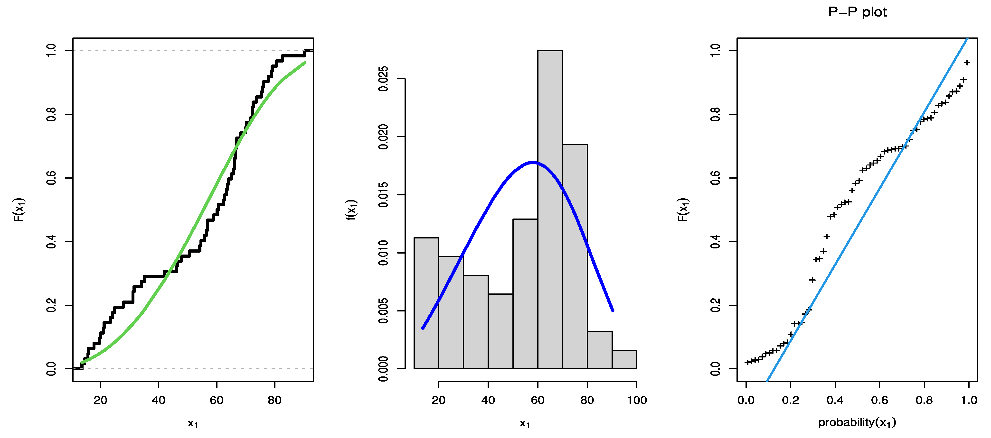
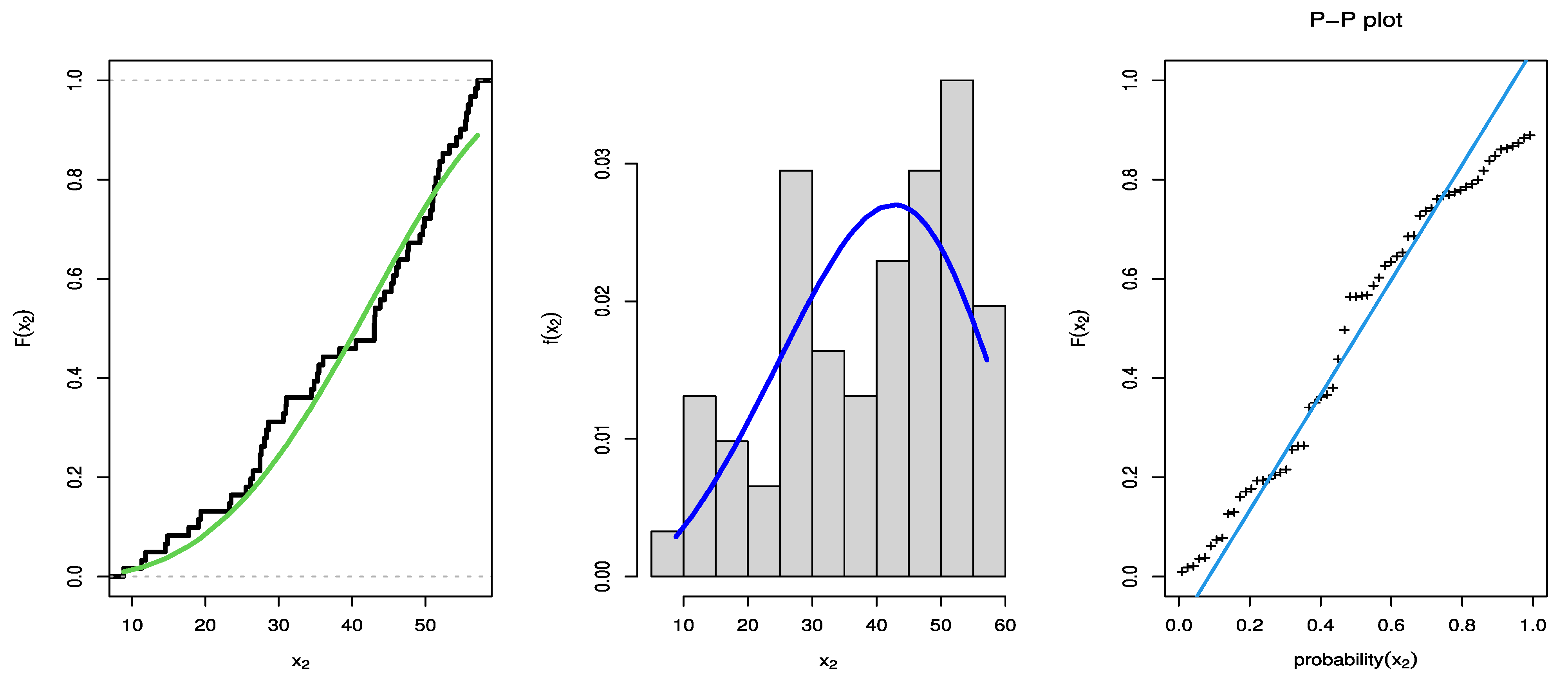
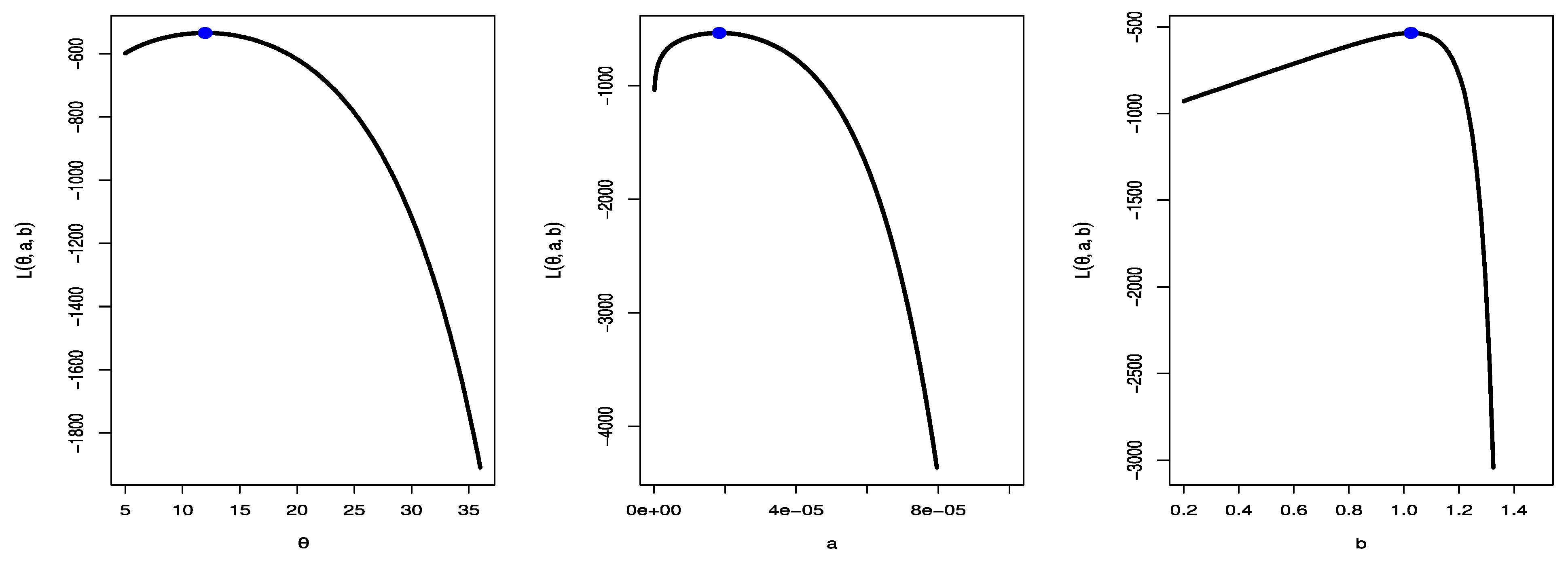
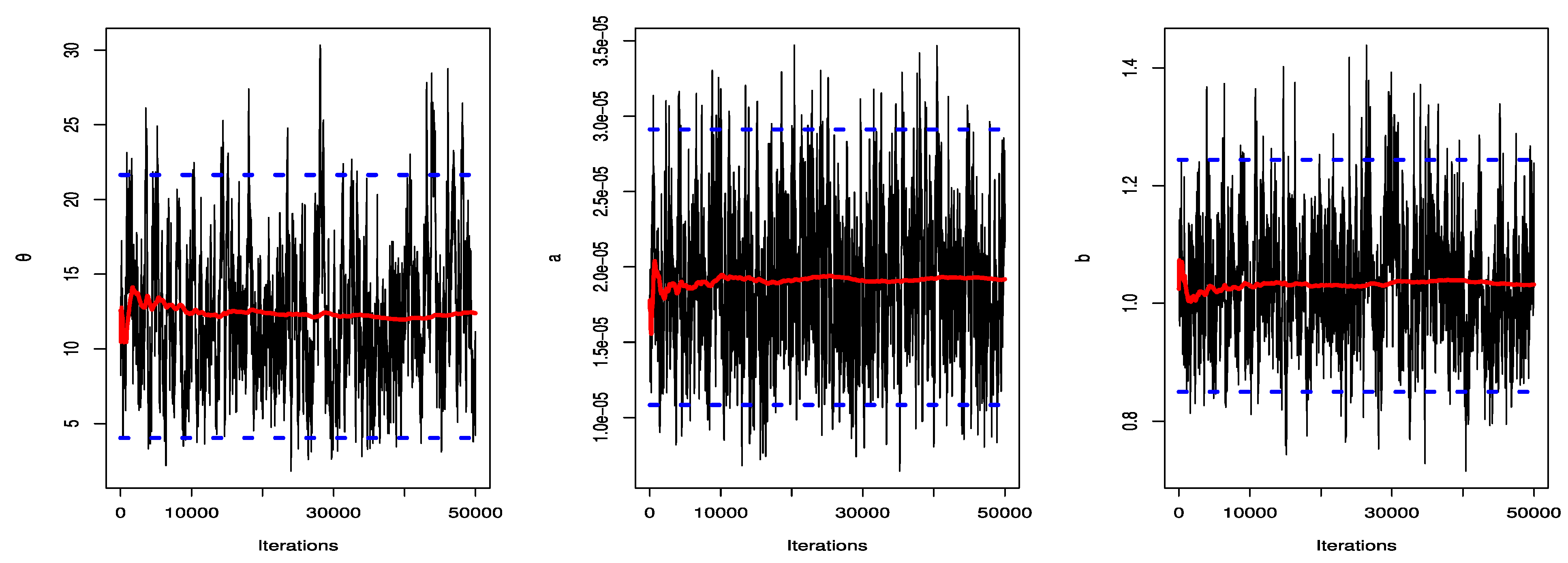
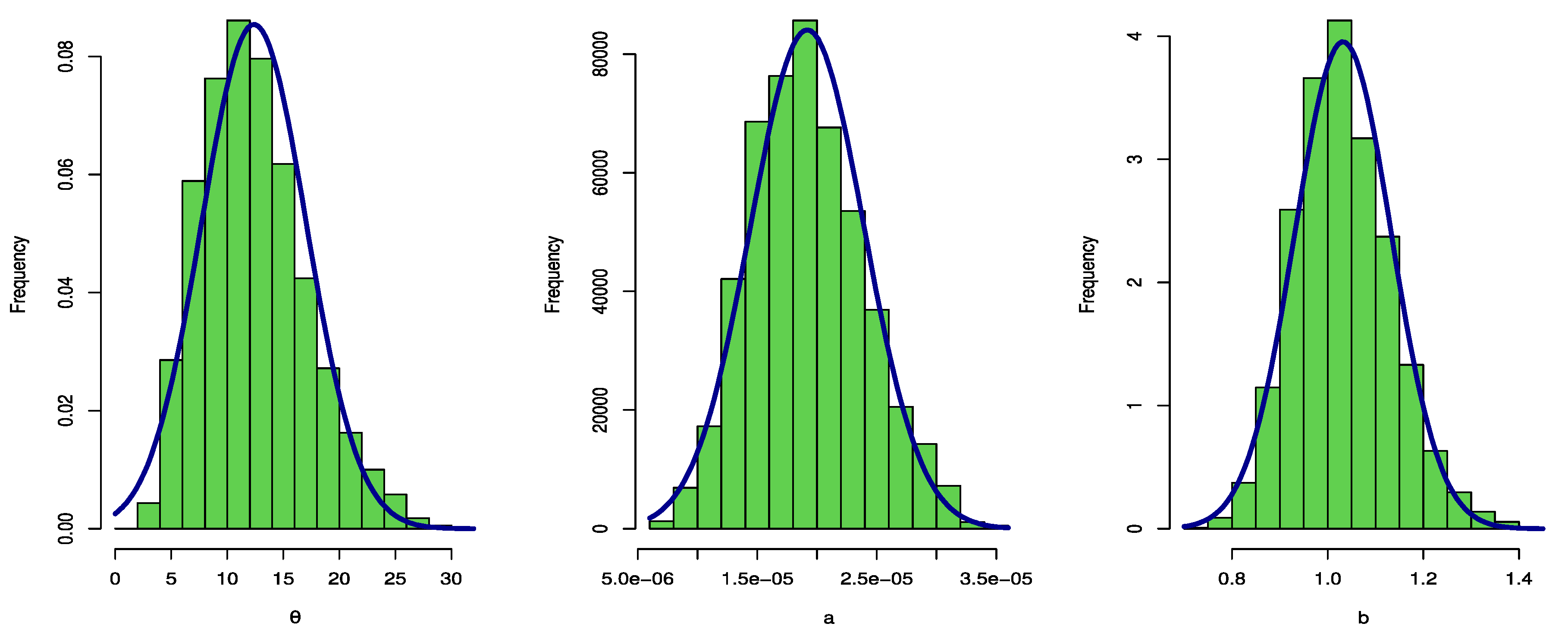
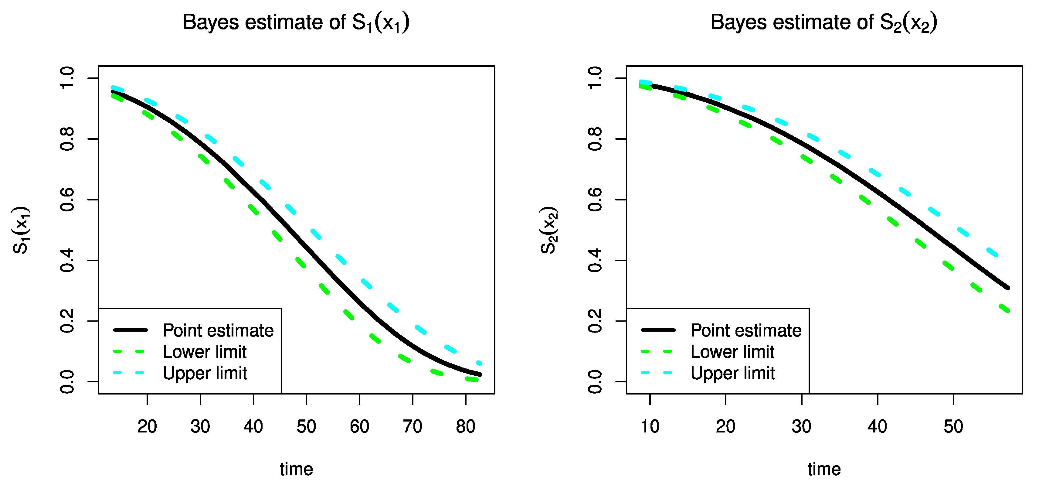
7. An Illustrative Example
8. Concluding Remarks
Author Contributions
Funding
Institutional Review Board Statement
Informed Consent Statement
Data Availability Statement
Conflicts of Interest
References
- Nadarajah, S.; Haghighi, F. An extension of the exponential distribution. Statistics 2011, 45, 543–558. [Google Scholar] [CrossRef]
- Khan, M.N.; Saboor, A.; Cordeiro, G.M.; Nazir, M. A weighted Nadarajah and Haghighi distribution. UPB Sci. Bull. Ser. A Appl. Math. Phys. 2018, 80, 133–140. [Google Scholar]
- Tahir, M.H.; Cordeiro, G.M.; Ali, S.; Dey, S.; Manzoor, A. The inverted Nadarajah–Haghighi distribution: Estimation methods and applications. J. Stat. Comput. Simul. 2018, 88, 2775–2798. [Google Scholar] [CrossRef]
- Chesneau, C.I.; Okorie, E.I.; Bakouch, H.S. A Skewed Nadarajah–Haghighi Distribution with Some Applications. J. Indian Soc. Probab. Stat. 2020, 21, 225–245. [Google Scholar] [CrossRef]
- Mansoor, M.; Tahir, M.H.; Alzaatreh, A.; Cordeiro, G.M. The Poisson Nadarajah—Haghighi Distribution: Properties and Applications to Lifetime Data. Int. J. Reliab. Qual. Saf. Eng. 2020, 27, 2050005. [Google Scholar] [CrossRef]
- Cohen, A.C. Progressively Censored Samples in Life Testing. Technometrics 1963, 5, 327. [Google Scholar] [CrossRef]
- Hofmann, G.; Cramer, E.; Balakrishnan, N.; Kunert, G. An asymptotic approach to progressive censoring. J. Stat. Plan. Inference 2005, 130, 207–227. [Google Scholar] [CrossRef]
- Lawless, J.F. Statistical Models and Methods for Lifetime Data; John Wiley and Sons: Hoboken, NJ, USA, 2003. [Google Scholar]
- Balakrishnan, N.; Aggarwala, R. Progressive Censoring: Theory, Methods, and Applications; Springer: Berlin/Heidelberg, Germany, 2000. [Google Scholar]
- Balakrishnan, N.; Sandhu, R.A. A simple simulation algorithm for generating progressive Type-II censored samples. Am. Stat. 1995, 199549, 229–230. [Google Scholar]
- Kundu, D.; Joarder, A. Analysis of Type-II progressively hybrid censored data. Comput. Stat. Data Anal. 2006, 50, 2509–2528. [Google Scholar] [CrossRef]
- Gupta, R.D.; Kundu, D. Hybrid censoring schemes with exponential failure distribution. Commun. Stat.-Theory Methods 1998, 27, 3065–3083. [Google Scholar] [CrossRef]
- Nelson, W.B. Accelerated Testing: Statistical Models, Test Plans, and Data Analysis; Wiley: New York, NY, USA, 1990. [Google Scholar]
- Miller, R.; Nelson, W. Optimum Simple Step-Stress Plans for Accelerated Life Testing. IEEE Trans. Reliab. 1983, R-32, 59–65. [Google Scholar] [CrossRef]
- Xiong, C. Step Stress Model with Threshold Parameter. J. Stat. Comput. Simul. 1999, 63, 349–360. [Google Scholar] [CrossRef]
- Park, S.-J.; Yum, B.-J. Optimal design of accelerated life tests under modified stress loading methods. J. Appl. Stat. 1998, 25, 41–62. [Google Scholar] [CrossRef]
- Lu, M.W.; Rudy, R.J. Step-stress accelerated test. Int. J. Mater. Prod. Technol. 2002, 17, 425–434. [Google Scholar] [CrossRef]
- El-Raheem, A.M.A.; Almetwally, E.M.; Mohamed, M.S.; Hafez, E.H. Accelerated life tests for modified Kies exponential lifetime distribution: Binomial removal, transformers turn insulation application and numerical results. AIMS Math. 2021, 6, 5222–5255. [Google Scholar] [CrossRef]
- Ahmadi, J.; Jozani, M.J.; Marchand, E.; Parsian, A. Bayes estimation based on k-record data from a general class of distributions under balanced type loss functions. J. Stat. Plan Inference 2009, 139, 1180–1189. [Google Scholar] [CrossRef]
- Ahmadi, J.; Jozani, M.J.; Marchand, E.; Parsian, A. Prediction of k-records from a general class of distributions under balanced type loss functions. Metrika 2008, 70, 19–33. [Google Scholar] [CrossRef]
- Ahmed, E.A. Bayesian estimation based on progressive Type-II censoring from two-parameter bathtub-shaped lifetime model: An Markov chain Monte Carlo approach. J. Appl. Stat. 2014, 41, 752–768. [Google Scholar] [CrossRef]
- Contreras-Reyes, J.E. Lerch distribution based on maximum nonsymmetric entropy principle: Application to Conway’s game of life cellular automaton. Chaos Solitons Fractals 2021, 151, 111272. [Google Scholar] [CrossRef]
- Almongy, H.; Alshenawy, F.; Almetwally, E.; Abdo, D. Applying Transformer Insulation Using Weibull Extended Distribution Based on Progressive Censoring Scheme. Axioms 2021, 10, 100. [Google Scholar] [CrossRef]
- Bantan, R.; Hassan, A.S.; Almetwally, E.; Elgarhy, M.; Jamal, F.; Chesneau, C.; Elsehetry, M. Bayesian Analysis in Partially Accelerated Life Tests for Weighted Lomax Distribution. Comput. Mater. Contin. 2021, 68, 2859–2875. [Google Scholar] [CrossRef]
- Alotaibi, R.; Al Mutairi, A.; Almetwally, E.M.; Park, C.; Rezk, H. Optimal Design for a Bivariate Step-Stress Accelerated Life Test with Alpha Power Exponential Distribution Based on Type-I Progressive Censored Samples. Symmetry 2022, 14, 830. [Google Scholar] [CrossRef]
- Alotaibi, R.; Khalifa, M.; Almetwally, E.M.; Ghosh, I.; Rezk, H. Classical and Bayesian Inference of a Mixture of Bivariate Exponentiated Exponential Model. J. Math. 2021, 2021, 1–20. [Google Scholar] [CrossRef]
- Tolba, A.H.; Almetwally, E.M.; Ramadan, D.A. Bayesian Estimation of A one Parameter Akshaya Distribution with Progressively Type II Censord Data. J. Stat. Appl. Probab. 2022, 11, 565–579. [Google Scholar]
- Chen, M.H.; Shao, Q.M. Monte Carlo estimation of Bayesian credible and HPD intervals. J. Comput. Graph. Stat. 1999, 8, 69–92. [Google Scholar]
- Tibshirani, R.; Efron, B. An Introduction to the Bootstrap; Chapman & Hall, Inc.: New York, NY, USA, 1993. [Google Scholar]
- R Core Team. A Language and Environment for Statistical Computing; R Foundation for Statistical Computing: Vienna, Austria, 2021. [Google Scholar]


| First Level | Second Level | |||
|---|---|---|---|---|
| Estimates | SE | Estimates | SE | |
| 3.3823 | 0.8429 | 2.6078 | 0.5590 | |
| a | ||||
| b | 1.3756 | 0.0320 | 1.6994 | 0.0507 |
| AIC | 554.7177 | 493.5818 | ||
| KSD | 0.1124 | 0.1113 | ||
| p-value | 0.3852 | 0.4362 | ||
| MLE | Bayesian | |||||||
|---|---|---|---|---|---|---|---|---|
| Estimates | SE | Lower | Upper | Estimates | SE | Lower | Upper | |
| θ | 11.9739 | 0.5590 | 0.0000 | 66.3388 | 12.3834 | 0.4691 | 4.0420 | 21.6353 |
| a | ||||||||
| b | 1.0260 | 0.0507 | 0.9979 | 1.0541 | 1.0322 | 0.0409 | 0.9997 | 1.0539 |
| AIC | 1074.528 | |||||||
Publisher’s Note: MDPI stays neutral with regard to jurisdictional claims in published maps and institutional affiliations. |
© 2022 by the authors. Licensee MDPI, Basel, Switzerland. This article is an open access article distributed under the terms and conditions of the Creative Commons Attribution (CC BY) license (https://creativecommons.org/licenses/by/4.0/).
Share and Cite
Alotaibi, R.; Alamri, F.S.; Almetwally, E.M.; Wang, M.; Rezk, H. Classical and Bayesian Inference of a Progressive-Stress Model for the Nadarajah–Haghighi Distribution with Type II Progressive Censoring and Different Loss Functions. Mathematics 2022, 10, 1602. https://doi.org/10.3390/math10091602
Alotaibi R, Alamri FS, Almetwally EM, Wang M, Rezk H. Classical and Bayesian Inference of a Progressive-Stress Model for the Nadarajah–Haghighi Distribution with Type II Progressive Censoring and Different Loss Functions. Mathematics. 2022; 10(9):1602. https://doi.org/10.3390/math10091602
Chicago/Turabian StyleAlotaibi, Refah, Faten S. Alamri, Ehab M. Almetwally, Min Wang, and Hoda Rezk. 2022. "Classical and Bayesian Inference of a Progressive-Stress Model for the Nadarajah–Haghighi Distribution with Type II Progressive Censoring and Different Loss Functions" Mathematics 10, no. 9: 1602. https://doi.org/10.3390/math10091602
APA StyleAlotaibi, R., Alamri, F. S., Almetwally, E. M., Wang, M., & Rezk, H. (2022). Classical and Bayesian Inference of a Progressive-Stress Model for the Nadarajah–Haghighi Distribution with Type II Progressive Censoring and Different Loss Functions. Mathematics, 10(9), 1602. https://doi.org/10.3390/math10091602