
Prototype of 3D Reliability Assessment Tool Based on Deep Learning for Edge OSS Computing


Abstract
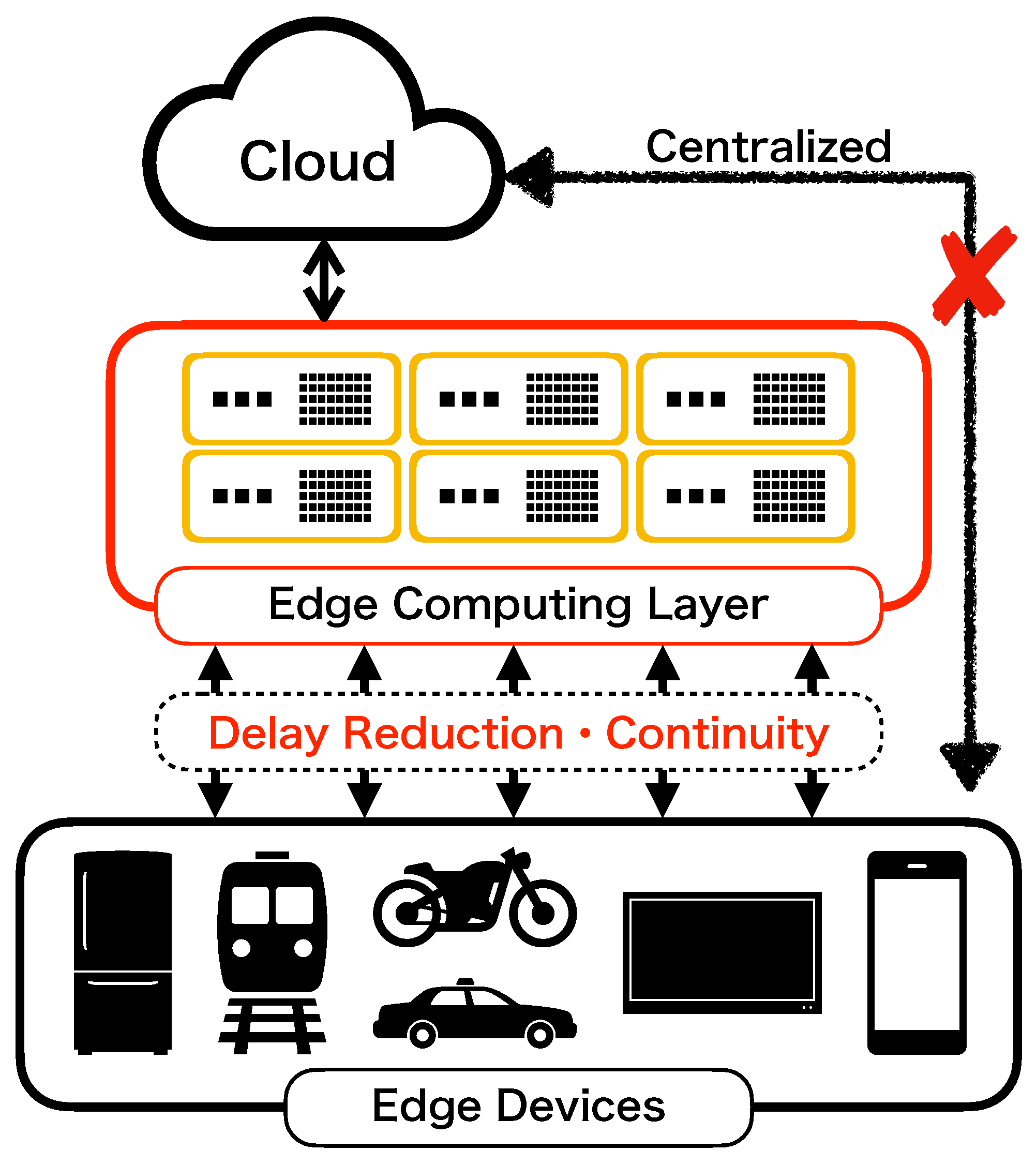
:1. Introduction
2. Data Preprocessing for Large-Scale OSS Fault Data
2.1. Related Work
- The software fault is caused as the result of a cause-and-effect relationship. Various data sets in terms of the cause-and-effect relationship are recorded on the bug-tracking system.
- We can comprehend the cause-and-effect relationship by using the big data on the bug-tracking system.
- The typical stochastic models are difficult to use, and the fault big data include many explanatory variables because of the problem of local minimum in terms of model parameters.
- The state of the art beyond the existing work in our method is to be able to use the fault big data. Moreover, our method is able to make an automatic feature extraction from the fault big data.
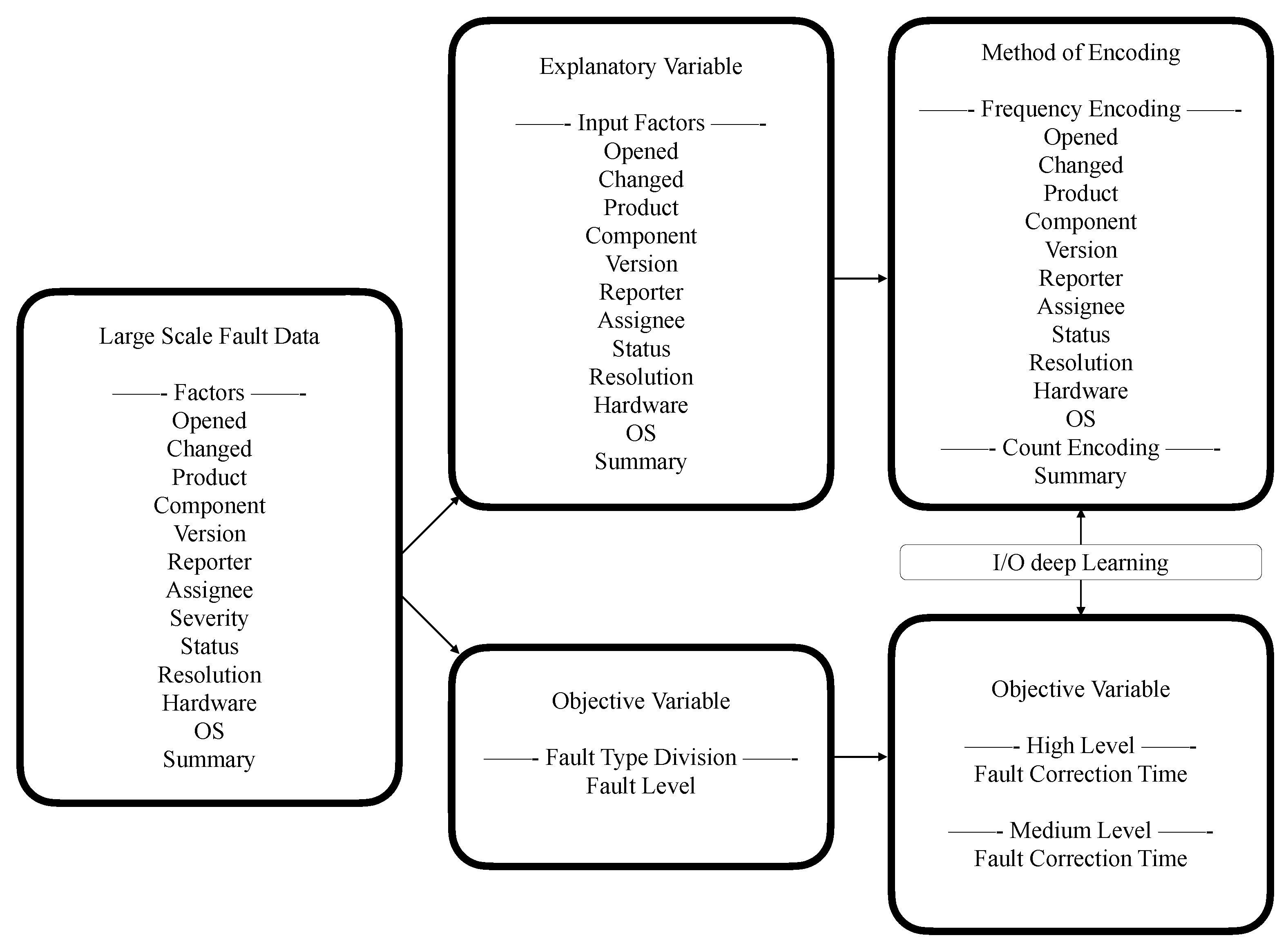
2.2. OSS Data Set
- Opened: is converted to the difference from the previous day, and this unit is day;
- Changed: is converted to the difference from the previous day, and this unit is day;
- Product: is converted to the values of the occurrence ratio for the product name by using the frequency encoding;
- Component: is converted to the values of the occurrence ratio for the component name by using the frequency encoding;
- Version: is converted to the frequency values of appearance for the same version number by using the frequency encoding;
- Reporter: is converted to the frequency values of appearance for the same nickname of reporter by using the frequency encoding;
- Assignee: is converted to the frequency values of appearance for the same nickname of assignee by using the frequency encoding;
- Severity: is converted to the values based on the same numbers of count for fault level by the frequency encoding;
- Status: is converted to the occurrence ratio of the status name by using the frequency encoding;
- Resolution: , as with what happened to the bugs, is converted to the occurrence ratio of the status name by using the frequency encoding;
- Hardware: is converted to numerical values in terms of hardware by the frequency encoding;
- OS: is also converted to numerical values in terms of the operating system by the frequency encoding;
- Summary: is converted to the number of words by using the count encoding;
2.3. Data Preprocessing
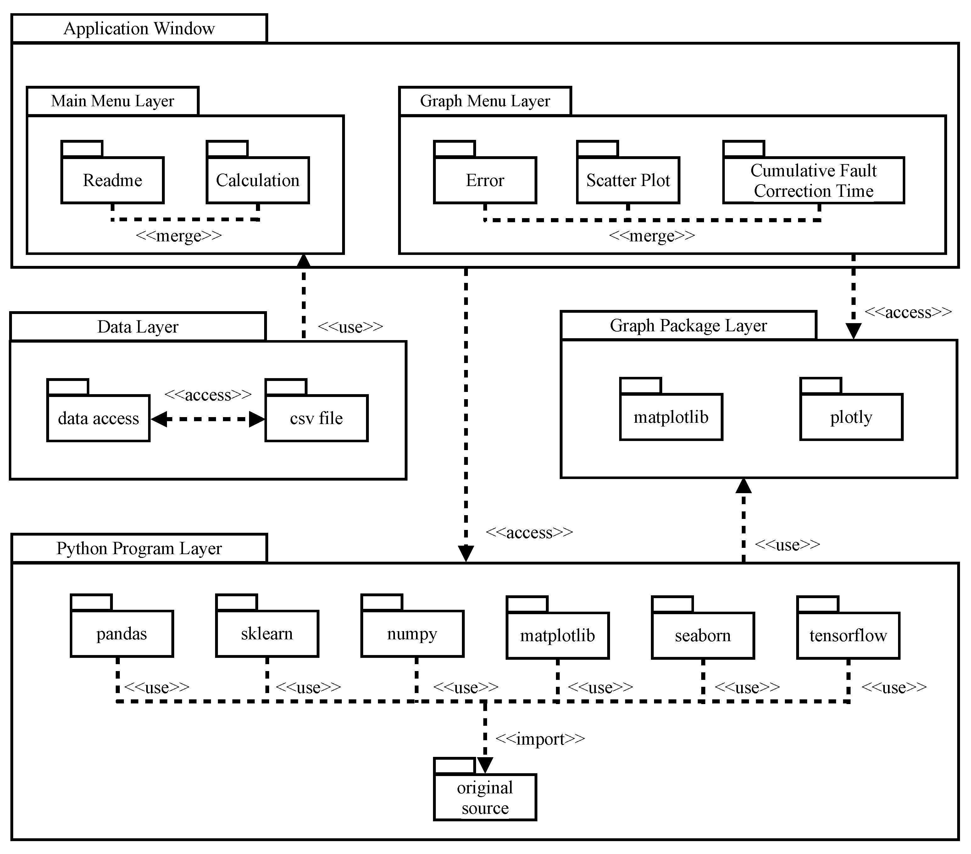
3. Development of Prototype Tool
- The user of the prototype starts from the main menu by running our application. In addition, the user completes data preprocessing.
- The user selects the calculation button. Then, the application window calls the Python program. In addition, the Python program imports the tensorflow package. Moreover, the proposed deep learning algorithm is executed by using Figure 3.
- After the completion of the learning phase, several reliability assessment measures are illustrated by selecting the graph button.
- ⦾
- Different programming languages (HTML, CSS, JavaScript, and Python).
- ⦾
- Dynamic links based on Node.js and the file system of OS, such as macOS, Windows, Linux, etc.
- ⦾
- There is a difference in the scale and language of the packages.
4. Performance Illustrations of the Developed 3D Application
4.1. Data Set for Edge OSS Computing
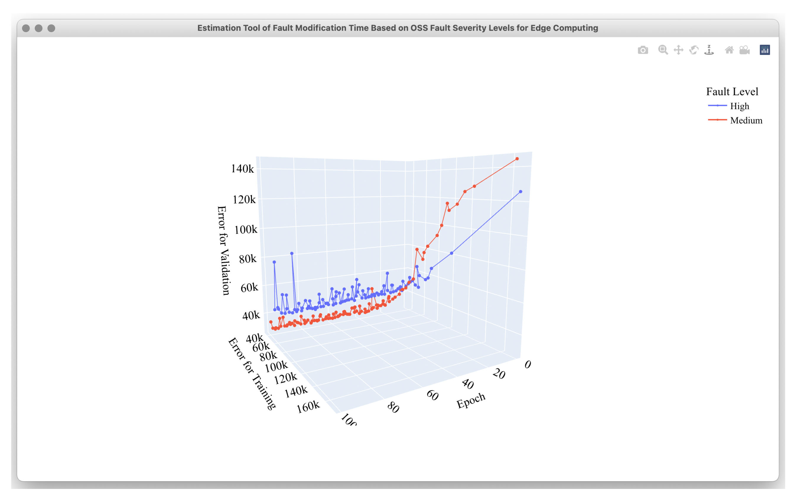
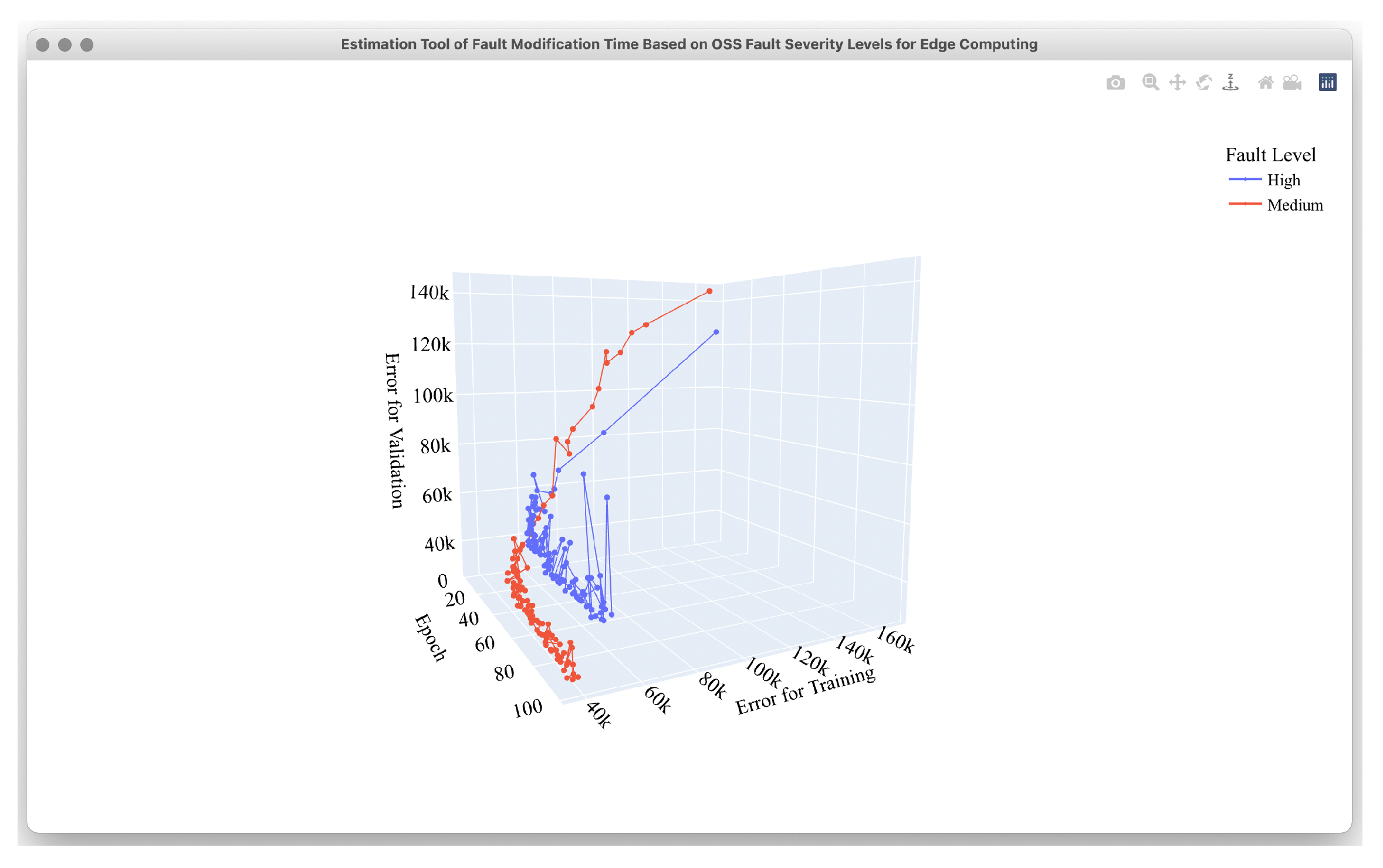
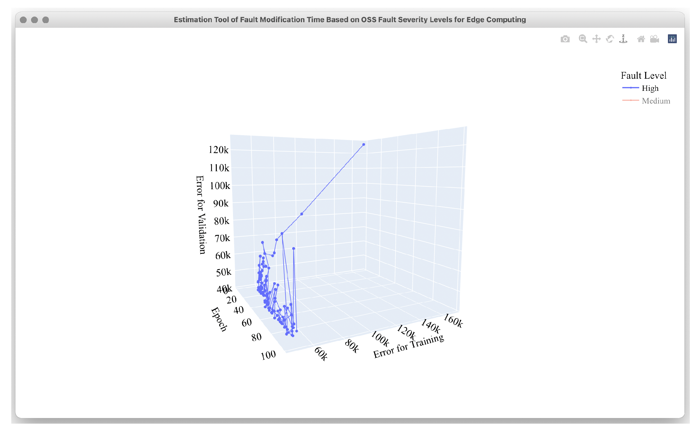
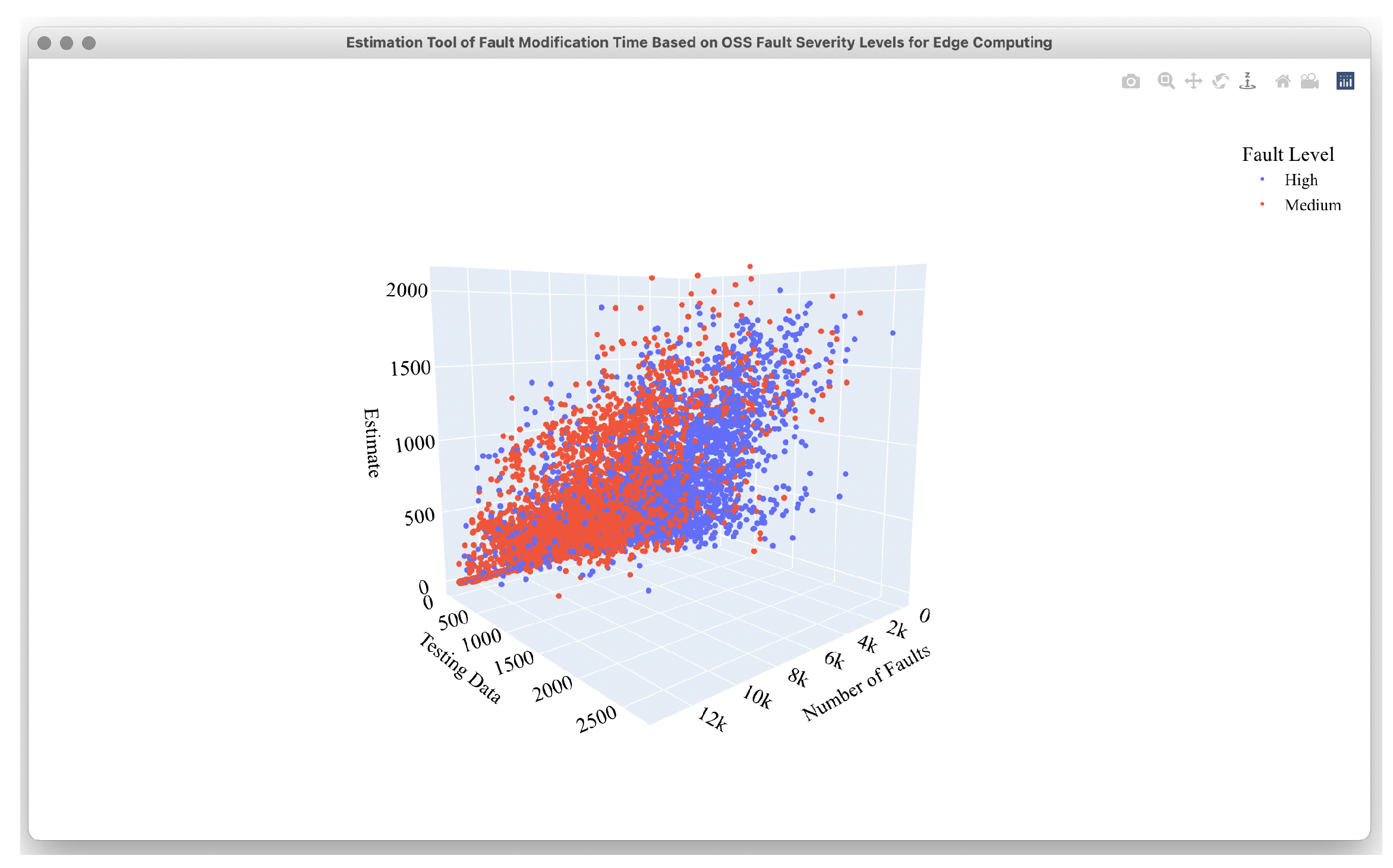
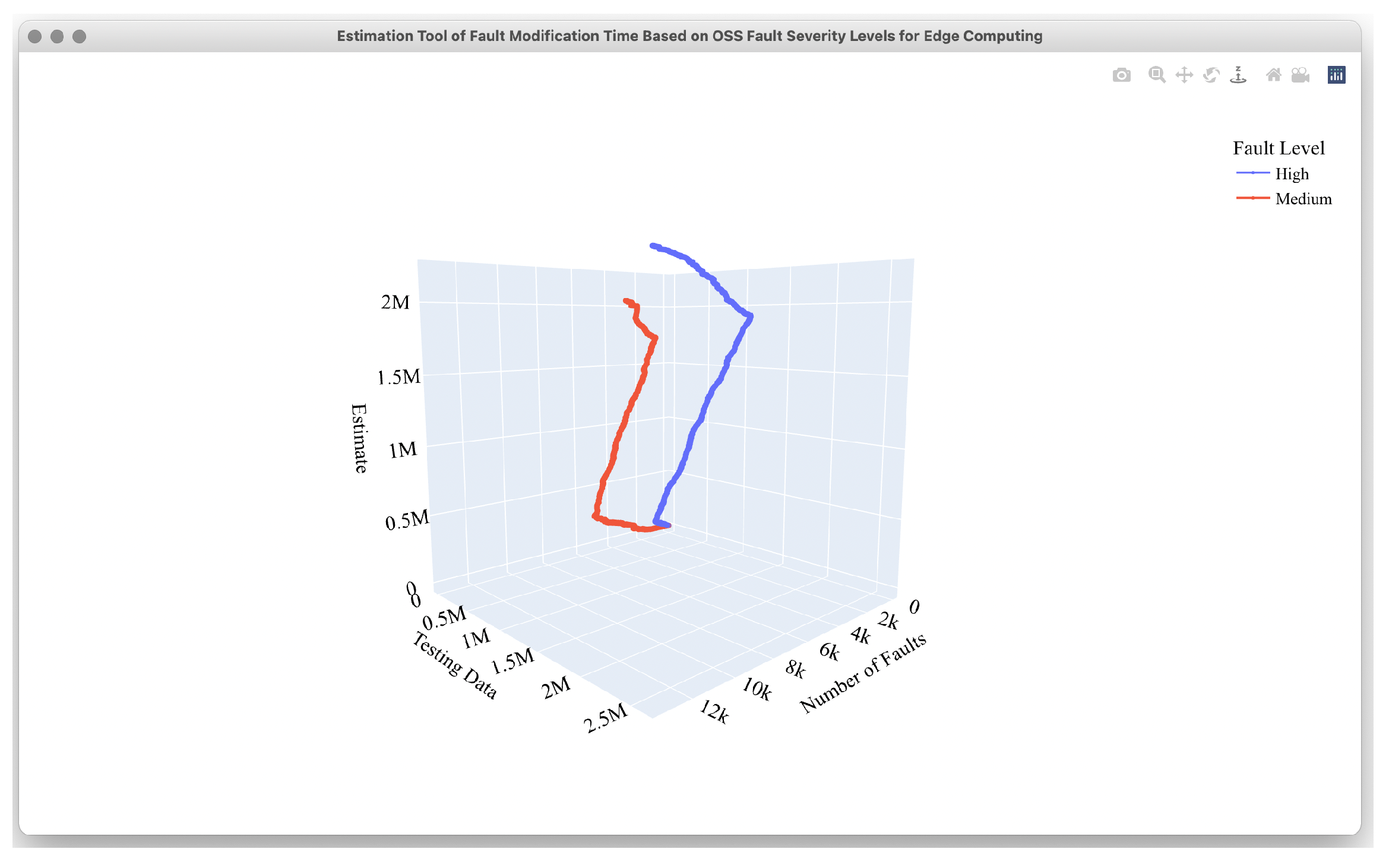
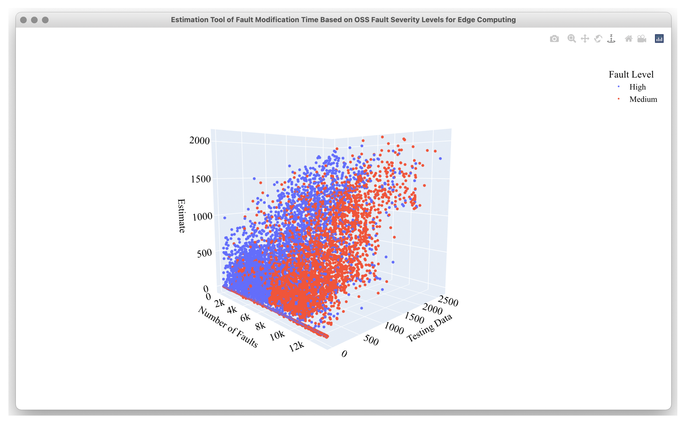
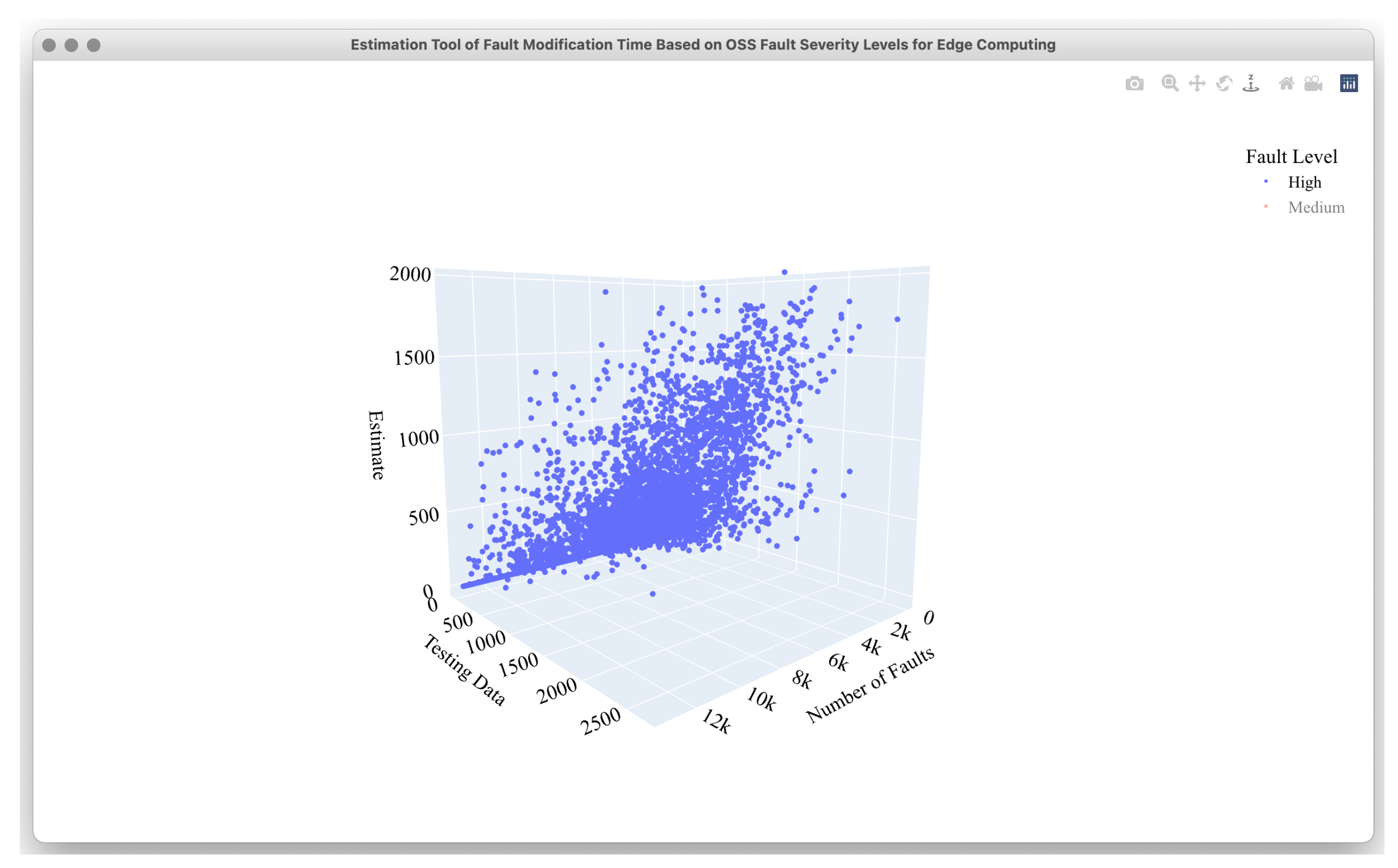
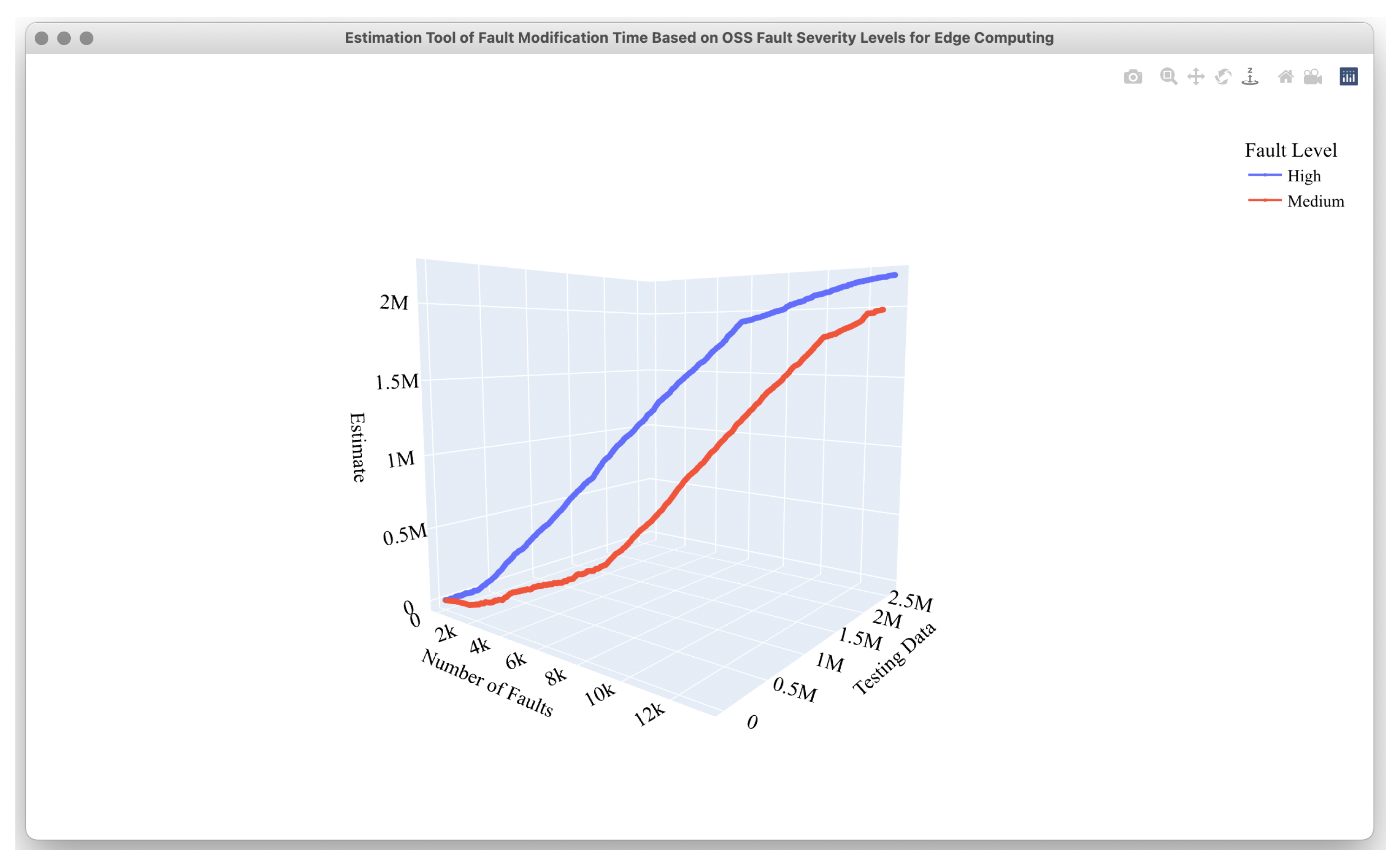
4.2. Estimation Results
4.3. Comparison Results
5. Concluding Remarks
- ⦾
- The comprehension of the trend of large-scale OSS fault levels as data preprocessing.
- ⦾
- The estimation of fault correction time based on two-stage deep learning.
- ⦾
- The development of a prototype as a reliability assessment tool based on deep learning that can be used by users who are not familiar with deep learning.
Author Contributions
Funding
Institutional Review Board Statement
Informed Consent Statement
Data Availability Statement
Acknowledgments
Conflicts of Interest
References
- Yamada, S.; Tamura, Y. OSS Reliability Measurement and Assessment; Springer International Publishing: Cham, Switzerland, 2016. [Google Scholar]
- Lyu, M.R. (Ed.) Handbook of Software Reliability Engineering; IEEE Computer Society Press: Los Alamitos, CA, USA, 1996. [Google Scholar]
- Yamada, S. Software Reliability Modeling: Fundamentals and Applications; Springer: Tokyo, Japan; Heidelberg, Germany, 2014. [Google Scholar]
- Kapur, P.K.; Pham, H.; Gupta, A.; Jha, P.C. Software Reliability Assessment with OR Applications; Springer: London, UK, 2011. [Google Scholar]
- Kingma, D.P.; Rezende, D.J.; Mohamed, S.; Welling, M. Semi-supervised learning with deep generative models. In Proceedings of the 27th International Conference on Neural Information Processing Systems, Montreal, QC, Canada, 8–13 December 2014. [Google Scholar]
- Sahu, K.; Srivastava, R.K. Revisiting software reliability, data management, analytics and innovation. In Advances in Intelligent Systems and Computing; Springer: Singapore, 2019; Volume 808. [Google Scholar]
- Sahu, K.; Srivastava, R.K. Soft computing approach for prediction of software reliability. ICIC Express Lett. 2018, 12, 1213–1222. [Google Scholar]
- Ji, C.; Su, X.; Qin, Z.; Nawaz, A. Probability analysis of construction risk based on noisy-or gate bayesian networks. Reliab. Eng. Syst. Saf. 2022, 217, 107974. [Google Scholar] [CrossRef]
- Sahu, K.; Srivastava, R.K. Needs and importance of reliability prediction: An industrial perspective. Inf. Sci. Lett. 2020, 9, 1–5. [Google Scholar]
- Sahu, K.; Srivastava, R.K. Predicting software bugs of newly and large datasets through a unified neuro-fuzzy approach: Reliability perspective. Adv. Math. Sci. J. 2021, 10, 543–555. [Google Scholar] [CrossRef]
- Türk, A.; Özkök, M. Shipyard location selection based on fuzzy AHP and TOPSIS. J. Intell. Fuzzy Syst. 2020, 39, 4557–4576. [Google Scholar] [CrossRef]
- Abuhamdah, A.; Boulila, W.; Jaradat, G.M.; Quteishat, A.M.; Alsmadi, M.K.; Almarashdeh, I.A. A novel population-based local search for nurse rostering problem. Int. J. Electr. Comput. Eng. 2021, 11, 471–480. [Google Scholar] [CrossRef]
- Ibrahim, I.M.; Mostafa, M.G.M.; El-Din, S.H.N.; Elgohary, R.; Faheem, H. A robust generic multi-authority attributes management system for cloud storage services. IEEE Trans. Cloud Comput. 2018, 9, 435–446. [Google Scholar] [CrossRef]
- Al-Said, A.A.; Andras, P. Scalability analysis comparisons of cloud-based software services. J. Cloud Comput. Adv. Syst. Appl. 2019, 8, 1–17. [Google Scholar] [CrossRef]
- Ozcan, M.O.; Odaci, F.; Ari, I. Remote debugging for containerized applications in edge computing environments. In Proceedings of the 2019 IEEE International Conference on Edge Computing (EDGE), Milan, Italy, 8–13 July 2019; pp. 30–32. [Google Scholar] [CrossRef]
- Hu, P.; Chen, W. Software-defined edge computing (SDEC): Principles, open system architecture and challenges. In Proceedings of the 2019 IEEE SmartWorld, Ubiquitous Intelligence & Computing, Advanced & Trusted Computing, Scalable Computing & Communications, Cloud & Big Data Computing, Internet of People and Smart City Innovation (SmartWorld/SCALCOM/UIC/ATC/CBDCom/IOP/SCI), Leicester, UK, 19–23 August 2019; pp. 8–16. [Google Scholar] [CrossRef]
- Alsenani, Y.; Crosby, G.; Velasco, T. SaRa: A stochastic model to estimate reliability of edge resources in volunteer cloud. In Proceedings of the 2018 IEEE International Conference on Edge Computing (EDGE), San Francisco, CA, USA, 2–7 July 2018; pp. 121–124. [Google Scholar] [CrossRef]
- Karunanithi, N.; Whitley, D.; Malaiya, Y.K. Using neural networks in reliability prediction. IEEE Softw. 1992, 9, 53–59. [Google Scholar] [CrossRef]
- Dohi, T.; Nishio, Y.; Osaki, S. Optimal software release scheduling based on artificial neural networks. Ann. Softw. Eng. 1999, 8, 167–185. [Google Scholar] [CrossRef]
- Blum, A.; Lafferty, J.; Rwebangira, M.R.; Reddy, R. Semi-supervised learning using randomized mincuts. In Proceedings of the International Conference on Machine Learning, Banff, AB, Canada, 4–8 July 2004. [Google Scholar]
- George, E.D.; Dong, Y.; Li, D.; Alex, A. Context-dependent pre-trained deep neural networks for large-vocabulary speech recognition. IEEE Trans. Audio Speech Lang. Process. 2012, 20, 30–42. [Google Scholar]
- Vincent, P.; Larochelle, H.; Lajoie, I.; Bengio, Y.; Manzagol, P.A. Stacked denoising autoencoders: Learning useful representations in a deep network with a local denoising criterion. J. Mach. Learn. Res. 2010, 11, 3371–3408. [Google Scholar]
- Martinez, H.P.; Bengio, Y.; Yannakakis, G.N. Learning deep physiological models of affect. IEEE Comput. Intell. Mag. 2013, 8, 20–33. [Google Scholar] [CrossRef] [Green Version]
- Hutchinson, B.; Deng, L.; Yu, D. Tensor deep stacking networks. IEEE Trans. Pattern Anal. Mach. Intell. 2013, 35, 1944–1957. [Google Scholar] [CrossRef] [PubMed]
- Kingma, D.P.; Ba, J.L. Adam: A method for stochastic optimizations. In Proceedings of the International Conference on Learning Representations, San Diego, CA, USA, 7–9 May 2015; pp. 1–15. [Google Scholar]
- Tamura, Y.; Yamada, S. Multi-dimensional software tool for OSS project management considering cloud with big data. Int. J. Reliab. Qual. Saf. Eng. 2018, 25, 1850014-1–1850014-16. [Google Scholar] [CrossRef]
- The OpenStack Project, Build the Future of Open Infrastructure. Available online: https://www.openstack.org/ (accessed on 24 February 2022).


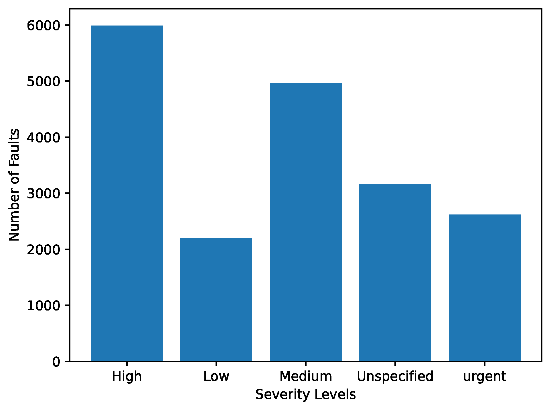
| Bug ID | Opened | Changed | Reporter | Product | Component | Status | Resolution | Hardware | OS | Severity | Version |
|---|---|---|---|---|---|---|---|---|---|---|---|
| 985361 | 2013/7/17 10:56 | 2014/1/9 19:40 | Jaroslav Henner | Red Hat OpenStack | openstack-packstack | CLOSED | ERRATA | x86_64 | Linux | medium | 3 |
| 1146938 | 2014/9/26 11:50 | 2016/4/26 13:26 | Sunil Thaha | Red Hat OpenStack | openstack-glance | CLOSED | CURRENTRELEASE | Unspecified | All | unspecified | 5.0 (RHEL 7) |
| 1155592 | 2014/10/22 12:52 | 2016/4/26 13:50 | Marian Krcmarik | Red Hat OpenStack | openstack-cinder | CLOSED | ERRATA | Unspecified | Unspecified | unspecified | 5.0 (RHEL 7) |
| 1157619 | 2014/10/27 11:31 | 2016/4/26 13:35 | Marko Myllynen | Red Hat OpenStack | openstack-cinder | CLOSED | CURRENTRELEASE | Unspecified | Unspecified | unspecified | 5.0 (RHEL 7) |
| 1163421 | 2014/11/12 16:42 | 2015/9/10 11:45 | Lon Hohberger | Red Hat OpenStack | openstack-trove | CLOSED | ERRATA | Unspecified | Unspecified | unspecified | 5.0 (RHEL 7) |
| 1169145 | 2014/11/30 17:56 | 2016/4/27 2:17 | bkopilov | Red Hat OpenStack | openstack-glance | CLOSED | CURRENTRELEASE | x86_64 | Linux | high | 6.0 (Juno) |
| 1170343 | 2014/12/3 21:01 | 2016/4/26 22:06 | Lon Hohberger | Red Hat OpenStack | openstack-glance | CLOSED | ERRATA | Unspecified | Unspecified | unspecified | 6.0 (Juno) |
| 1174760 | 2014/12/16 12:37 | 2016/4/26 22:58 | Dafna Ron | Red Hat OpenStack | openstack-cinder | CLOSED | DUPLICATE | x86_64 | Linux | urgent | 6.0 (Juno) |
| 1184349 | 2015/1/21 7:35 | 2016/4/26 18:02 | bkopilov | Red Hat OpenStack | openstack-cinder | CLOSED | NOTABUG | x86_64 | Linux | high | 6.0 (Juno) |
| 1186395 | 2015/1/27 15:36 | 2016/4/26 15:16 | Red Hat OpenStack | openstack-cinder | CLOSED | WONTFIX | Unspecified | Unspecified | unspecified | 5.0 (RHEL 7) | |
| 1209584 | 2015/4/7 17:13 | 2015/5/12 4:04 | Luigi Toscano | Red Hat OpenStack | openstack-trove | CLOSED | ERRATA | Unspecified | Unspecified | unspecified | 6.0 (Juno) |
| 1254711 | 2015/8/18 17:29 | 2016/4/26 17:48 | Lon Hohberger | Red Hat OpenStack | openstack-glance | CLOSED | ERRATA | Unspecified | Unspecified | unspecified | 5.0 (RHEL 7) |
| 1254718 | 2015/8/18 17:31 | 2016/4/26 14:59 | Lon Hohberger | Red Hat OpenStack | openstack-glance | CLOSED | ERRATA | Unspecified | Unspecified | unspecified | 5.0 (RHEL 6) |
| 1304111 | 2016/2/2 22:17 | 2016/12/14 15:22 | Dustin Schoenbrun | Red Hat OpenStack | openstack-manila-ui | CLOSED | ERRATA | Unspecified | Unspecified | high | 8.0 (Liberty) |
| 1314821 | 2016/3/4 15:45 | 2016/4/26 15:10 | Flavio Percoco | Red Hat OpenStack | openstack-glance | CLOSED | ERRATA | Unspecified | Unspecified | unspecified | 8.0 (Liberty) |
| 1333884 | 2016/5/6 14:37 | 2016/8/11 12:19 | Harry Rybacki | Red Hat OpenStack | openstack-tempest | CLOSED | ERRATA | Unspecified | Unspecified | unspecified | 9.0 (Mitaka) |
| 1346749 | 2016/6/15 9:54 | 2016/8/11 12:25 | Anshul Behl | Red Hat OpenStack | openstack-ironic | CLOSED | ERRATA | Unspecified | Unspecified | unspecified | 9.0 (Mitaka) |
| 1441796 | 2017/4/12 18:12 | 2017/4/12 18:13 | Red Hat OpenStack | openstack-ironic-inspector | CLOSED | NOTABUG | Unspecified | Unspecified | unspecified | 7.0 (Kilo) | |
| 1455490 | 2017/5/25 10:24 | 2020/7/16 9:39 | Eduard Barrera | Red Hat OpenStack | openstack-tripleo | CLOSED | DUPLICATE | Unspecified | Unspecified | unspecified | 10.0 (Newton) |
| 1544713 | 2018/2/13 11:14 | 2019/9/9 16:48 | Punit Kundal | Red Hat OpenStack | openstack-nova | CLOSED | INSUFFICIENT_DATA | Unspecified | Unspecified | medium | 10.0 (Newton) |
| 1545722 | 2018/2/15 14:26 | 2021/3/11 17:11 | David Vallee Delisle | Red Hat OpenStack | openstack-nova | CLOSED | WONTFIX | Unspecified | Unspecified | unspecified | 10.0 (Newton) |
| 1545809 | 2018/2/15 15:38 | 2021/3/11 17:12 | KOSAL RAJ I | Red Hat OpenStack | openstack-nova | CLOSED | INSUFFICIENT_DATA | Unspecified | Unspecified | high | 10.0 (Newton) |
| 1547969 | 2018/2/22 12:38 | 2019/9/9 13:10 | Madhur Gupta | Red Hat OpenStack | openstack-nova | CLOSED | DUPLICATE | x86_64 | Linux | medium | 10.0 (Newton) |
| 1551911 | 2018/3/6 7:09 | 2019/9/9 15:56 | Petersingh Anburaj | Red Hat OpenStack | openstack-nova | CLOSED | WONTFIX | Unspecified | Unspecified | high | 11.0 (Ocata) |
| 1552761 | 2018/3/7 16:47 | 2019/9/9 13:22 | Stephen Gordon | Red Hat OpenStack | openstack-nova | CLOSED | NOTABUG | Unspecified | Unspecified | unspecified | 10.0 (Newton) |
| 1554341 | 2018/3/12 13:42 | 2019/9/9 14:42 | Carlos Camacho | Red Hat OpenStack | openstack-nova | CLOSED | WONTFIX | All | All | high | 10.0 (Newton) |
| 1557383 | 2018/3/16 14:02 | 2019/9/9 15:05 | David Vallee Delisle | Red Hat OpenStack | openstack-nova | CLOSED | INSUFFICIENT_DATA | Unspecified | Unspecified | low | 12.0 (Pike) |
| 1561008 | 2018/3/27 12:37 | 2019/9/9 17:08 | Maxim Babushkin | Red Hat OpenStack | openstack-nova | CLOSED | NOTABUG | Unspecified | Unspecified | urgent | 13.0 (Queens) |
| 1561636 | 2018/3/28 15:52 | 2019/9/9 16:19 | Alexander Chuzhoy | Red Hat OpenStack | openstack-nova | CLOSED | NOTABUG | Unspecified | Unspecified | unspecified | 13.0 (Queens) |
| 1562154 | 2018/3/29 16:06 | 2019/9/9 16:17 | Dariusz Wojewdzki | Red Hat OpenStack | openstack-nova | CLOSED | NOTABUG | Unspecified | Unspecified | high | 10.0 (Newton) |
| 1563646 | 2018/4/4 11:45 | 2019/9/9 14:37 | Gurenko Alex | Red Hat OpenStack | openstack-nova | CLOSED | DUPLICATE | Unspecified | Unspecified | medium | 13.0 (Queens) |
| 1565532 | 2018/4/10 8:56 | 2019/9/9 15:43 | Arie Bregman | Red Hat OpenStack | openstack-nova | CLOSED | DUPLICATE | Unspecified | Unspecified | high | 12.0 (Pike) |
| 1565533 | 2018/4/10 8:58 | 2019/9/9 15:30 | Arie Bregman | Red Hat OpenStack | openstack-nova | CLOSED | DUPLICATE | Unspecified | Unspecified | high | 11.0 (Ocata) |
| 1567601 | 2018/4/15 9:54 | 2019/9/9 13:31 | Noam Manos | Red Hat OpenStack | openstack-nova | CLOSED | INSUFFICIENT_DATA | Unspecified | Unspecified | unspecified | 13.0 (Queens) |
| 1568262 | 2018/4/17 4:51 | 2019/10/16 0:49 | Pradipta Kumar Sahoo | Red Hat OpenStack | openstack-nova | CLOSED | WONTFIX | x86_64 | Linux | medium | 12.0 (Pike) |
| 1569107 | 2018/4/18 15:43 | 2020/12/21 19:40 | David Hill | Red Hat OpenStack | openstack-nova | CLOSED | NOTABUG | Unspecified | Unspecified | unspecified | 10.0 (Newton) |
| 1569238 | 2018/4/18 20:53 | 2020/12/21 19:33 | Siggy Sigwald | Red Hat OpenStack | openstack-nova | CLOSED | NOTABUG | x86_64 | Linux | high | 10.0 (Newton) |
| 1571499 | 2018/4/25 2:20 | 2019/9/9 13:50 | Sai Sindhur Malleni | Red Hat OpenStack | openstack-nova | CLOSED | INSUFFICIENT_DATA | Unspecified | Unspecified | unspecified | 13.0 (Queens) |
| 1572547 | 2018/4/27 9:58 | 2020/12/21 19:38 | Red Hat OpenStack | openstack-nova | CLOSED | WONTFIX | Unspecified | Linux | high | 10.0 (Newton) | |
| 1572833 | 2018/4/28 2:16 | 2019/9/9 15:57 | Lars Kellogg-Stedman | Red Hat OpenStack | openstack-nova | CLOSED | NOTABUG | Unspecified | Unspecified | unspecified | 12.0 (Pike) |
| 1573269 | 2018/4/30 17:20 | 2019/9/9 13:54 | Lars Kellogg-Stedman | Red Hat OpenStack | openstack-nova | CLOSED | DUPLICATE | Unspecified | Unspecified | unspecified | 12.0 (Pike) |
| 1574465 | 2018/5/3 11:30 | 2020/12/21 19:36 | Red Hat OpenStack | openstack-nova | CLOSED | NOTABUG | x86_64 | Linux | urgent | 13.0 (Queens) | |
| 1575753 | 2018/5/7 19:47 | 2020/12/21 19:36 | bigswitch | Red Hat OpenStack | openstack-nova | CLOSED | NOTABUG | Unspecified | Unspecified | unspecified | 10.0 (Newton) |
| 1579136 | 2018/5/17 4:06 | 2020/12/21 19:36 | Red Hat OpenStack | openstack-nova | CLOSED | NOTABUG | Unspecified | Unspecified | high | 13.0 (Queens) | |
| 1582845 | 2018/5/27 11:33 | 2019/9/9 13:22 | Red Hat OpenStack | openstack-nova | CLOSED | NOTABUG | Unspecified | Unspecified | unspecified | 13.0 (Queens) | |
| 1584118 | 2018/5/30 10:33 | 2020/12/21 19:36 | Andre | Red Hat OpenStack | openstack-nova | CLOSED | WONTFIX | Unspecified | Unspecified | unspecified | unspecified |
| 1584268 | 2018/5/30 15:21 | 2019/9/9 16:21 | Dan Smith | Red Hat OpenStack | openstack-nova | CLOSED | DUPLICATE | Unspecified | Unspecified | unspecified | 15.0 (Stein) |
| 1586267 | 2018/6/5 20:19 | 2019/9/9 15:29 | Tim Quinlan | Red Hat OpenStack | openstack-nova | CLOSED | INSUFFICIENT_DATA | x86_64 | Linux | low | 10.0 (Newton) |
| 1591091 | 2018/6/14 4:18 | 2019/9/9 14:17 | Anil Dhingra | Red Hat OpenStack | openstack-nova | CLOSED | WONTFIX | All | Linux | medium | 10.0 (Newton) |
| 1592123 | 2018/6/17 13:43 | 2019/9/9 14:00 | Arkady Shtempler | Red Hat OpenStack | openstack-nova | CLOSED | WONTFIX | Unspecified | Unspecified | unspecified | 13.0 (Queens) |
| 1593751 | 2018/6/21 14:07 | 2020/12/21 19:45 | Artom Lifshitz | Red Hat OpenStack | openstack-nova | CLOSED | NOTABUG | Unspecified | Unspecified | unspecified | 13.0 (Queens) |
| 1594454 | 2018/6/23 5:25 | 2019/9/9 14:26 | Cody Swanson | Red Hat OpenStack | openstack-nova | CLOSED | NOTABUG | x86_64 | Linux | medium | 10.0 (Newton) |
| 1596706 | 2018/6/29 13:52 | 2019/9/9 13:26 | Mikel Olasagasti | Red Hat OpenStack | openstack-nova | CLOSED | WONTFIX | Unspecified | Unspecified | unspecified | 10.0 (Newton) |
| 1598624 | 2018/7/6 2:56 | 2019/9/9 17:05 | Meiyan Zheng | Red Hat OpenStack | openstack-nova | CLOSED | WONTFIX | Unspecified | Unspecified | unspecified | 10.0 (Newton) |
| 1600641 | 2018/7/12 16:37 | 2019/9/9 16:16 | Rajini Karthik | Red Hat OpenStack | openstack-nova | CLOSED | NOTABUG | Unspecified | Unspecified | urgent | 13.0 (Queens) |
| 1601123 | 2018/7/14 0:18 | 2019/9/9 14:09 | Stan Toporek | Red Hat OpenStack | openstack-nova | CLOSED | NOTABUG | Unspecified | Unspecified | urgent | 7.0 (Kilo) |
| 1607467 | 2018/7/23 15:31 | 2019/9/9 16:50 | Masaki Furuta ( RH ) | Red Hat OpenStack | openstack-nova | CLOSED | INSUFFICIENT_DATA | Unspecified | Unspecified | unspecified | 12.0 (Pike) |
| 1608487 | 2018/7/25 15:48 | 2019/9/9 13:41 | David Gurtner | Red Hat OpenStack | openstack-nova | CLOSED | INSUFFICIENT_DATA | Unspecified | Unspecified | unspecified | 13.0 (Queens) |
| 1608531 | 2018/7/25 17:57 | 2019/9/9 15:52 | Jeya ganesh babu J | Red Hat OpenStack | openstack-nova | CLOSED | DUPLICATE | Unspecified | Linux | high | 13.0 (Queens) |
| 1615736 | 2018/8/14 7:03 | 2019/9/9 15:28 | Gyanendra Kumar | Red Hat OpenStack | openstack-nova | CLOSED | WONTFIX | Unspecified | All | high | 13.0 (Queens) |
| 1616398 | 2018/8/15 19:30 | 2019/9/9 15:28 | Andreas Karis | Red Hat OpenStack | openstack-nova | CLOSED | CANTFIX | Unspecified | Unspecified | unspecified | 10.0 (Newton) |
| 1620195 | 2018/8/22 16:15 | 2019/9/9 15:33 | Federico Iezzi | Red Hat OpenStack | openstack-nova | CLOSED | DUPLICATE | Unspecified | Unspecified | unspecified | 13.0 (Queens) |
| 1622950 | 2018/8/28 8:48 | 2019/11/20 14:19 | Anil Dhingra | Red Hat OpenStack | openstack-nova | CLOSED | NOTABUG | Unspecified | Unspecified | high | 10.0 (Newton) |
| 1624262 | 2018/8/31 6:50 | 2019/9/9 13:09 | Yurii Prokulevych | Red Hat OpenStack | openstack-nova | CLOSED | NOTABUG | Unspecified | Unspecified | unspecified | 8.0 (Liberty) |
| 1624266 | 2018/8/31 7:02 | 2020/12/21 19:33 | Yurii Prokulevych | Red Hat OpenStack | openstack-nova | CLOSED | DUPLICATE | Unspecified | Unspecified | unspecified | 8.0 (Liberty) |
| 1624521 | 2018/8/31 21:51 | 2019/9/9 13:06 | Archit Modi | Red Hat OpenStack | openstack-nova | CLOSED | DUPLICATE | Unspecified | Unspecified | unspecified | 13.0 (Queens) |
| 1625319 | 2018/9/4 16:06 | 2019/9/9 14:00 | Andreas Karis | Red Hat OpenStack | openstack-nova | CLOSED | INSUFFICIENT_DATA | Unspecified | Unspecified | unspecified | 12.0 (Pike) |
| 1632028 | 2018/9/23 13:17 | 2019/9/9 16:17 | David Hill | Red Hat OpenStack | openstack-nova | CLOSED | INSUFFICIENT_DATA | x86_64 | All | low | 10.0 (Newton) |
| 1633804 | 2018/9/27 19:04 | 2019/9/9 15:38 | Danylo Kholodov | Red Hat OpenStack | openstack-nova | CLOSED | NOTABUG | Unspecified | Unspecified | medium | 14.0 (Rocky) |
| 1635568 | 2018/10/3 9:29 | 2019/9/9 14:10 | Vadim Khitrin | Red Hat OpenStack | openstack-nova | CLOSED | DUPLICATE | Unspecified | Unspecified | urgent | 13.0 (Queens) |
| 1635666 | 2018/10/3 13:03 | 2019/9/9 14:33 | Archit Modi | Red Hat OpenStack | openstack-nova | CLOSED | WONTFIX | Unspecified | Unspecified | unspecified | 11.0 (Ocata) |
| 1638095 | 2018/10/10 16:26 | 2019/9/9 13:18 | Red Hat OpenStack | openstack-nova | CLOSED | NOTABUG | Unspecified | Unspecified | unspecified | 14.0 (Rocky) | |
| 1638368 | 2018/10/11 12:03 | 2019/9/9 16:08 | Red Hat OpenStack | openstack-nova | CLOSED | WONTFIX | Unspecified | Unspecified | urgent | 10.0 (Newton) | |
| 1638923 | 2018/10/12 20:15 | 2020/12/21 19:33 | Red Hat OpenStack | openstack-nova | CLOSED | NOTABUG | Unspecified | Unspecified | high | 13.0 (Queens) | |
| 1639334 | 2018/10/15 13:43 | 2019/9/9 13:30 | Sasha Smolyak | Red Hat OpenStack | openstack-nova | CLOSED | NOTABUG | Unspecified | Unspecified | unspecified | 14.0 (Rocky) |
| 1639423 | 2018/10/15 17:02 | 2019/9/9 13:17 | Sai Sindhur Malleni | Red Hat OpenStack | openstack-nova | CLOSED | NOTABUG | Unspecified | Unspecified | unspecified | 13.0 (Queens) |
| 1641597 | 2018/10/22 10:00 | 2019/9/9 14:25 | Mike Abrams | Red Hat OpenStack | openstack-nova | CLOSED | NOTABUG | x86_64 | Linux | unspecified | 14.0 (Rocky) |
| 1641610 | 2018/10/22 10:50 | 2019/9/9 15:53 | Mike Abrams | Red Hat OpenStack | openstack-nova | CLOSED | DUPLICATE | x86_64 | Linux | unspecified | 14.0 (Rocky) |
| 1642047 | 2018/10/23 13:17 | 2020/6/5 4:13 | Eduard Barrera | Red Hat OpenStack | openstack-nova | CLOSED | NOTABUG | Unspecified | Unspecified | unspecified | 12.0 (Pike) |
| 1642070 | 2018/10/23 14:11 | 2020/12/21 19:38 | Noam Manos | Red Hat OpenStack | openstack-nova | CLOSED | NOTABUG | Unspecified | Unspecified | high | 13.0 (Queens) |
| 1643147 | 2018/10/25 15:17 | 2019/9/9 15:21 | Raoul Scarazzini | Red Hat OpenStack | openstack-nova | CLOSED | DUPLICATE | Unspecified | Unspecified | unspecified | 14.0 (Rocky) |
| 1643419 | 2018/10/26 8:20 | 2019/12/3 20:16 | Alex Stupnikov | Red Hat OpenStack | openstack-nova | CLOSED | WONTFIX | Unspecified | Unspecified | high | 13.0 (Queens) |
| 1643420 | 2018/10/26 8:22 | 2019/9/9 14:54 | Alex Stupnikov | Red Hat OpenStack | openstack-nova | CLOSED | WONTFIX | Unspecified | Unspecified | high | 12.0 (Pike) |
| 1643784 | 2018/10/28 17:26 | 2019/9/9 15:07 | Alex Stupnikov | Red Hat OpenStack | openstack-nova | CLOSED | NOTABUG | x86_64 | Linux | medium | 10.0 (Newton) |
| 1644549 | 2018/10/31 6:25 | 2020/12/21 19:36 | Prasad Mukhedkar | Red Hat OpenStack | openstack-nova | CLOSED | INSUFFICIENT_DATA | x86_64 | Linux | high | 12.0 (Pike) |
| 1646447 | 2018/11/5 14:58 | 2019/9/9 13:10 | Archit Modi | Red Hat OpenStack | openstack-nova | CLOSED | NOTABUG | Unspecified | Unspecified | unspecified | 14.0 (Rocky) |
| 1646457 | 2018/11/5 15:08 | 2019/9/9 13:11 | Archit Modi | Red Hat OpenStack | openstack-nova | CLOSED | NOTABUG | Unspecified | Unspecified | unspecified | 14.0 (Rocky) |
| 1649937 | 2018/11/14 20:58 | 2020/12/21 19:35 | Alexander Chuzhoy | Red Hat OpenStack | openstack-nova | CLOSED | WORKSFORME | Unspecified | Unspecified | unspecified | 14.0 (Rocky) |
| 1650192 | 2018/11/15 14:56 | 2019/9/9 15:49 | Lars Kellogg-Stedman | Red Hat OpenStack | openstack-nova | CLOSED | NOTABUG | Unspecified | Unspecified | unspecified | 13.0 (Queens) |
| 1652197 | 2018/11/21 16:33 | 2019/9/9 13:44 | Vadim Khitrin | Red Hat OpenStack | openstack-nova | CLOSED | NOTABUG | Unspecified | Unspecified | unspecified | 14.0 (Rocky) |
| 1654288 | 2018/11/28 12:06 | 2018/12/13 12:38 | Red Hat OpenStack | openstack-tripleo-common | CLOSED | NOTABUG | Unspecified | Unspecified | high | 14.0 (Rocky) | |
| 1655476 | 2018/12/3 9:19 | 2019/9/9 15:48 | Eduard Barrera | Red Hat OpenStack | openstack-nova | CLOSED | WONTFIX | Unspecified | Unspecified | unspecified | 15.0 (Stein) |
| 1655480 | 2018/12/3 9:32 | 2019/9/9 13:18 | Yurii Prokulevych | Red Hat OpenStack | openstack-nova | CLOSED | DUPLICATE | Unspecified | Unspecified | unspecified | 14.0 (Rocky) |
| 1655510 | 2018/12/3 10:40 | 2019/9/9 16:54 | Eduard Barrera | Red Hat OpenStack | openstack-nova | CLOSED | INSUFFICIENT_DATA | Unspecified | Unspecified | unspecified | 13.0 (Queens) |
| 1655989 | 2018/12/4 11:39 | 2019/9/9 13:51 | Red Hat OpenStack | openstack-nova | CLOSED | INSUFFICIENT_DATA | x86_64 | Linux | medium | 10.0 (Newton) | |
| 1657391 | 2018/12/7 21:18 | 2019/9/9 17:07 | Red Hat OpenStack | openstack-nova | CLOSED | NOTABUG | Unspecified | Unspecified | unspecified | 14.0 (Rocky) | |
| 1658105 | 2018/12/11 9:28 | 2019/9/9 13:22 | Arkady Shtempler | Red Hat OpenStack | openstack-nova | CLOSED | NOTABUG | Unspecified | Linux | medium | 14.0 (Rocky) |
| 1658151 | 2018/12/11 11:55 | 2020/12/21 19:38 | Noam Manos | Red Hat OpenStack | openstack-nova | CLOSED | NOTABUG | Unspecified | Unspecified | urgent | 14.0 (Rocky) |
| 1659539 | 2018/12/14 16:02 | 2019/9/9 13:11 | Krish Raghuram | Red Hat OpenStack | openstack-nova | CLOSED | DEFERRED | x86_64 | Linux | high | 16.0 (Train) |
| 1661190 | 2018/12/20 10:50 | 2019/9/9 13:59 | Noam Manos | Red Hat OpenStack | openstack-nova | CLOSED | NOTABUG | Unspecified | Unspecified | medium | 14.0 (Rocky) |
| Bug ID | Opened | Changed | Reporter | Product | Component | Status | Resolution | Hardware | OS | Severity | Version | Summary |
|---|---|---|---|---|---|---|---|---|---|---|---|---|
| 985361 | 0.005716067 | 1 | 0.0463 | 1 | 0.4148 | 0.1595 | 0.2304 | 0.1164 | 0.0204 | 60 | ||
| 1146938 | 436.0377315 | 837.7402662 | 0.000103928 | 1 | 0.0249 | 1 | 0.0892 | 0.7671 | 0.0292 | 0.2721 | 0.0567 | 53 |
| 1155592 | 26.04289352 | 0.016435185 | 0.001974641 | 1 | 0.0806 | 1 | 0.4148 | 0.7671 | 0.7401 | 0.2721 | 0.0567 | 65 |
| 1157619 | 4.943796296 | 0 | 0.001870713 | 1 | 0.0806 | 1 | 0.0892 | 0.7671 | 0.7401 | 0.2721 | 0.0567 | 47 |
| 1163421 | 16.21612269 | 0 | 0.014446061 | 1 | 0.0024 | 1 | 0.4148 | 0.7671 | 0.7401 | 0.2721 | 0.0567 | 50 |
| 1169145 | 18.05128472 | 229.605544 | 0.006027853 | 1 | 0.0249 | 1 | 0.0892 | 0.1595 | 0.2304 | 0.3469 | 0.0469 | 55 |
| 1170343 | 3.128715278 | 0 | 0.014446061 | 1 | 0.0249 | 1 | 0.4148 | 0.7671 | 0.7401 | 0.2721 | 0.0469 | 35 |
| 1174760 | 12.64994213 | 0.03587963 | 0.010600707 | 1 | 0.0806 | 1 | 0.134 | 0.1595 | 0.2304 | 0.2311 | 0.0469 | 130 |
| 1184349 | 35.78974537 | 0 | 0.006027853 | 1 | 0.0806 | 1 | 0.1728 | 0.1595 | 0.2304 | 0.3469 | 0.0469 | 68 |
| 1186395 | 6.334305556 | 0 | 0 | 1 | 0.0806 | 1 | 0.0752 | 0.7671 | 0.7401 | 0.2721 | 0.0567 | 96 |
| 1209584 | 70.06747685 | 0 | 0.003325712 | 1 | 0.0024 | 1 | 0.4148 | 0.7671 | 0.7401 | 0.2721 | 0.0469 | 78 |
| 1254711 | 133.0113194 | 350.5725579 | 0.014446061 | 1 | 0.0249 | 1 | 0.4148 | 0.7671 | 0.7401 | 0.2721 | 0.0567 | 35 |
| 1254718 | 0.001238426 | 0 | 0.014446061 | 1 | 0.0249 | 1 | 0.4148 | 0.7671 | 0.7401 | 0.2721 | 0.0174 | 35 |
| 1304111 | 168.1981829 | 232.0158218 | 0.001662856 | 1 | 0.0009 | 1 | 0.4148 | 0.7671 | 0.7401 | 0.3469 | 0.0685 | 63 |
| 1314821 | 30.72837963 | 0 | 0.001870713 | 1 | 0.0249 | 1 | 0.4148 | 0.7671 | 0.7401 | 0.2721 | 0.0685 | 32 |
| 1333884 | 62.9521412 | 106.8807755 | 0.002702141 | 1 | 0.0097 | 1 | 0.4148 | 0.7671 | 0.7401 | 0.2721 | 0.0399 | 107 |
| 1346749 | 39.80396991 | 0.00443287 | 0.000831428 | 1 | 0.0263 | 1 | 0.4148 | 0.7671 | 0.7401 | 0.2721 | 0.0399 | 68 |
| 1441796 | 301.3458333 | 244.2415972 | 0 | 1 | 0.0062 | 1 | 0.1728 | 0.7671 | 0.7401 | 0.2721 | 0.0824 | 8 |
| 1455490 | 42.67511574 | 1190.643229 | 0.012783205 | 1 | 0.0397 | 1 | 0.134 | 0.7671 | 0.7401 | 0.2721 | 0.1183 | 101 |
| 1544713 | 264.0345718 | 0 | 0.001870713 | 1 | 0.1365 | 1 | 0.0409 | 0.7671 | 0.7401 | 0.1164 | 0.1183 | 75 |
| 1545722 | 2.132893519 | 549.0164583 | 0.003741426 | 1 | 0.1365 | 1 | 0.0752 | 0.7671 | 0.7401 | 0.2721 | 0.1183 | 110 |
| 1545809 | 0.05056713 | 6.94444E-05 | 0.002286427 | 1 | 0.1365 | 1 | 0.0409 | 0.7671 | 0.7401 | 0.3469 | 0.1183 | 41 |
| 1547969 | 6.874780093 | 0 | 0.000727499 | 1 | 0.1365 | 1 | 0.134 | 0.1595 | 0.2304 | 0.1164 | 0.1183 | 59 |
| 1551911 | 11.77181713 | 0.114930556 | 0.000207857 | 1 | 0.1365 | 1 | 0.0752 | 0.7671 | 0.7401 | 0.3469 | 0.0419 | 37 |
| 1552761 | 1.401342593 | 0 | 0.007482852 | 1 | 0.1365 | 1 | 0.1728 | 0.7671 | 0.7401 | 0.2721 | 0.1183 | 38 |
| 1554341 | 4.870891204 | 0.055185185 | 0.001039285 | 1 | 0.1365 | 1 | 0.0752 | 0.0724 | 0.0292 | 0.3469 | 0.1183 | 31 |
| 1557383 | 4.014224537 | 0.016006944 | 0.003741426 | 1 | 0.1365 | 1 | 0.0409 | 0.7671 | 0.7401 | 0.0335 | 0.0611 | 50 |
| 1561008 | 10.94109954 | 0.085821759 | 0.00207857 | 1 | 0.1365 | 1 | 0.1728 | 0.7671 | 0.7401 | 0.2311 | 0.1391 | 59 |
| 1561636 | 1.135023148 | 0 | 0.019746414 | 1 | 0.1365 | 1 | 0.1728 | 0.7671 | 0.7401 | 0.2721 | 0.1391 | 126 |
| 1562154 | 1.010023148 | 0 | 0.000727499 | 1 | 0.1365 | 1 | 0.1728 | 0.7671 | 0.7401 | 0.3469 | 0.1183 | 28 |
| 1563646 | 5.818923611 | 0 | 0.003013926 | 1 | 0.1365 | 1 | 0.134 | 0.7671 | 0.7401 | 0.1164 | 0.1391 | 55 |
| 1565532 | 5.882407407 | 0.045810185 | 0.008626065 | 1 | 0.1365 | 1 | 0.134 | 0.7671 | 0.7401 | 0.3469 | 0.0611 | 189 |
| 1565533 | 0.001759259 | 0 | 0.008626065 | 1 | 0.1365 | 1 | 0.134 | 0.7671 | 0.7401 | 0.3469 | 0.0419 | 189 |
| 1567601 | 5.038449074 | 0 | 0.001558927 | 1 | 0.1365 | 1 | 0.0409 | 0.7671 | 0.7401 | 0.2721 | 0.1391 | 56 |
| 1568262 | 1.789571759 | 36.47054398 | 0.002390355 | 1 | 0.1365 | 1 | 0.0752 | 0.1595 | 0.2304 | 0.1164 | 0.0611 | 39 |
| 1569107 | 1.453032407 | 432.7852546 | 0.014030347 | 1 | 0.1365 | 1 | 0.1728 | 0.7671 | 0.7401 | 0.2721 | 0.1183 | 126 |
| 1569238 | 0.214930556 | 0 | 0.004261068 | 1 | 0.1365 | 1 | 0.1728 | 0.1595 | 0.2304 | 0.3469 | 0.1183 | 70 |
| 1571499 | 6.22755787 | 0 | 0.003845354 | 1 | 0.1365 | 1 | 0.0409 | 0.7671 | 0.7401 | 0.2721 | 0.1391 | 42 |
| 1572547 | 2.317615741 | 469.2414699 | 0 | 1 | 0.1365 | 1 | 0.0752 | 0.7671 | 0.2304 | 0.3469 | 0.1183 | 54 |
| 1572833 | 0.679189815 | 0 | 0.004884639 | 1 | 0.1365 | 1 | 0.1728 | 0.7671 | 0.7401 | 0.2721 | 0.0611 | 65 |
| 1573269 | 2.62775463 | 0 | 0.004884639 | 1 | 0.1365 | 1 | 0.134 | 0.7671 | 0.7401 | 0.2721 | 0.0611 | 77 |
| 1574465 | 2.757268519 | 469.2371875 | 0 | 1 | 0.1365 | 1 | 0.1728 | 0.1595 | 0.2304 | 0.2311 | 0.1391 | 35 |
| 1575753 | 4.344849537 | 0.000428241 | 0.003221783 | 1 | 0.1365 | 1 | 0.1728 | 0.7671 | 0.7401 | 0.2721 | 0.1183 | 80 |
| 1579136 | 9.346736111 | 0 | 0 | 1 | 0.1365 | 1 | 0.1728 | 0.7671 | 0.7401 | 0.3469 | 0.1391 | 55 |
| 1582845 | 10.31016204 | 0 | 0 | 1 | 0.1365 | 1 | 0.1728 | 0.7671 | 0.7401 | 0.2721 | 0.1391 | 28 |
| 1584118 | 2.958611111 | 469.2595023 | 0.001662856 | 1 | 0.1365 | 1 | 0.0752 | 0.7671 | 0.7401 | 0.2721 | 0.0471 | 44 |
| 1584268 | 0.200104167 | 0 | 0.000727499 | 1 | 0.1365 | 1 | 0.134 | 0.7671 | 0.7401 | 0.2721 | 0.0417 | 64 |
| 1586267 | 6.206446759 | 0 | 0.000519642 | 1 | 0.1365 | 1 | 0.0409 | 0.1595 | 0.2304 | 0.0335 | 0.1183 | 52 |
| 1591091 | 8.333009259 | 0 | 0.00135107 | 1 | 0.1365 | 1 | 0.0752 | 0.0724 | 0.2304 | 0.1164 | 0.1183 | 81 |
| 1592123 | 3.392222222 | 0 | 0.000935356 | 1 | 0.1365 | 1 | 0.0752 | 0.7671 | 0.7401 | 0.2721 | 0.1391 | 73 |
| 1593751 | 4.016793981 | 469.2395602 | 0.001974641 | 1 | 0.1365 | 1 | 0.1728 | 0.7671 | 0.7401 | 0.2721 | 0.1391 | 23 |
| 1594454 | 1.637523148 | 0 | 0.000415714 | 1 | 0.1365 | 1 | 0.1728 | 0.1595 | 0.2304 | 0.1164 | 0.1183 | 56 |
| 1596706 | 6.351828704 | 0 | 0.000623571 | 1 | 0.1365 | 1 | 0.0752 | 0.7671 | 0.7401 | 0.2721 | 0.1183 | 81 |
| 1598624 | 6.544340278 | 0.151666667 | 0.001662856 | 1 | 0.1365 | 1 | 0.0752 | 0.7671 | 0.7401 | 0.2721 | 0.1183 | 124 |
| 1600641 | 6.570659722 | 0 | 0.003741426 | 1 | 0.1365 | 1 | 0.1728 | 0.7671 | 0.7401 | 0.2311 | 0.1391 | 60 |
| 1601123 | 1.320127315 | 0 | 0.000935356 | 1 | 0.1365 | 1 | 0.1728 | 0.7671 | 0.7401 | 0.2311 | 0.0824 | 40 |
| 1607467 | 9.633449074 | 0.111770833 | 0.001039285 | 1 | 0.1365 | 1 | 0.0409 | 0.7671 | 0.7401 | 0.2721 | 0.0611 | 47 |
| 1608487 | 2.012071759 | 0 | 0.000519642 | 1 | 0.1365 | 1 | 0.0409 | 0.7671 | 0.7401 | 0.2721 | 0.1391 | 94 |
| 1608531 | 0.089618056 | 0.091030093 | 0.000103928 | 1 | 0.1365 | 1 | 0.134 | 0.7671 | 0.2304 | 0.3469 | 0.1391 | 64 |
| 1615736 | 19.54592593 | 0 | 0.001143213 | 1 | 0.1365 | 1 | 0.0752 | 0.7671 | 0.0292 | 0.3469 | 0.1391 | 82 |
| 1616398 | 1.518356481 | 0 | 0.012991062 | 1 | 0.1365 | 1 | 0.0048 | 0.7671 | 0.7401 | 0.2721 | 0.1183 | 87 |
| 1620195 | 6.865219907 | 0.003831019 | 0.000831428 | 1 | 0.1365 | 1 | 0.134 | 0.7671 | 0.7401 | 0.2721 | 0.1391 | 59 |
| 1622950 | 5.689363426 | 71.94840278 | 0.00135107 | 1 | 0.1365 | 1 | 0.1728 | 0.7671 | 0.7401 | 0.3469 | 0.1183 | 41 |
| 1624262 | 2.917986111 | 0 | 0.016420703 | 1 | 0.1365 | 1 | 0.1728 | 0.7671 | 0.7401 | 0.2721 | 0.0685 | 79 |
| 1624266 | 0.008032407 | 469.266331 | 0.016420703 | 1 | 0.1365 | 1 | 0.134 | 0.7671 | 0.7401 | 0.2721 | 0.0685 | 72 |
| 1624521 | 0.617905093 | 0 | 0.005404282 | 1 | 0.1365 | 1 | 0.134 | 0.7671 | 0.7401 | 0.2721 | 0.1391 | 67 |
| 1625319 | 3.759837963 | 0.037256944 | 0.012991062 | 1 | 0.1365 | 1 | 0.0409 | 0.7671 | 0.7401 | 0.2721 | 0.0611 | 113 |
| 1632028 | 18.88309028 | 0.095555556 | 0.014030347 | 1 | 0.1365 | 1 | 0.0409 | 0.1595 | 0.0292 | 0.0335 | 0.1183 | 63 |
| 1633804 | 4.240555556 | 0 | 0.000103928 | 1 | 0.1365 | 1 | 0.1728 | 0.7671 | 0.7401 | 0.1164 | 0.051 | 57 |
| 1635568 | 5.600960648 | 0 | 0.001870713 | 1 | 0.1365 | 1 | 0.134 | 0.7671 | 0.7401 | 0.2311 | 0.1391 | 71 |
| 1635666 | 0.148738426 | 0.016469907 | 0.005404282 | 1 | 0.1365 | 1 | 0.0752 | 0.7671 | 0.7401 | 0.2721 | 0.0419 | 63 |
| 1638095 | 7.140706019 | 0 | 0 | 1 | 0.1365 | 1 | 0.1728 | 0.7671 | 0.7401 | 0.2721 | 0.051 | 55 |
| 1638368 | 0.817847222 | 0.118148148 | 0 | 1 | 0.1365 | 1 | 0.0752 | 0.7671 | 0.7401 | 0.2311 | 0.1183 | 175 |
| 1638923 | 1.341018519 | 469.1426389 | 0 | 1 | 0.1365 | 1 | 0.1728 | 0.7671 | 0.7401 | 0.3469 | 0.1391 | 56 |
| 1639334 | 2.728402778 | 0 | 0.003637497 | 1 | 0.1365 | 1 | 0.1728 | 0.7671 | 0.7401 | 0.2721 | 0.051 | 92 |
| 1639423 | 0.137685185 | 0 | 0.003845354 | 1 | 0.1365 | 1 | 0.1728 | 0.7671 | 0.7401 | 0.2721 | 0.1391 | 40 |
| 1641597 | 6.706840278 | 0.047384259 | 0.003325712 | 1 | 0.1365 | 1 | 0.1728 | 0.1595 | 0.2304 | 0.2721 | 0.051 | 106 |
| 1641610 | 0.034861111 | 0.060983796 | 0.003325712 | 1 | 0.1365 | 1 | 0.134 | 0.1595 | 0.2304 | 0.2721 | 0.051 | 64 |
| 1642047 | 1.102013889 | 269.5134144 | 0.012783205 | 1 | 0.1365 | 1 | 0.1728 | 0.7671 | 0.7401 | 0.2721 | 0.0611 | 61 |
| 1642070 | 0.037928241 | 199.6425694 | 0.001558927 | 1 | 0.1365 | 1 | 0.1728 | 0.7671 | 0.7401 | 0.3469 | 0.1391 | 67 |
| 1643147 | 2.045821759 | 0 | 0.000831428 | 1 | 0.1365 | 1 | 0.134 | 0.7671 | 0.7401 | 0.2721 | 0.051 | 71 |
| 1643419 | 0.710335648 | 85.20469907 | 0.003949283 | 1 | 0.1365 | 1 | 0.0752 | 0.7671 | 0.7401 | 0.3469 | 0.1391 | 100 |
| 1643420 | 0.001585648 | 0 | 0.003949283 | 1 | 0.1365 | 1 | 0.0752 | 0.7671 | 0.7401 | 0.3469 | 0.0611 | 100 |
| 1643784 | 2.377222222 | 0.009259259 | 0.003949283 | 1 | 0.1365 | 1 | 0.1728 | 0.1595 | 0.2304 | 0.1164 | 0.1183 | 90 |
| 1644549 | 2.541446759 | 469.1866088 | 0.000207857 | 1 | 0.1365 | 1 | 0.0409 | 0.1595 | 0.2304 | 0.3469 | 0.0611 | 45 |
| 1646447 | 5.355775463 | 0 | 0.005404282 | 1 | 0.1365 | 1 | 0.1728 | 0.7671 | 0.7401 | 0.2721 | 0.051 | 73 |
| 1646457 | 0.007094907 | 0.001331019 | 0.005404282 | 1 | 0.1365 | 1 | 0.1728 | 0.7671 | 0.7401 | 0.2721 | 0.051 | 68 |
| 1649937 | 9.242893519 | 469.266412 | 0.019746414 | 1 | 0.1365 | 1 | 0.0267 | 0.7671 | 0.7401 | 0.2721 | 0.051 | 144 |
| 1650192 | 0.748969907 | 0 | 0.004884639 | 1 | 0.1365 | 1 | 0.1728 | 0.7671 | 0.7401 | 0.2721 | 0.1391 | 53 |
| 1652197 | 6.067291667 | 0 | 0.001870713 | 1 | 0.1365 | 1 | 0.1728 | 0.7671 | 0.7401 | 0.2721 | 0.051 | 61 |
| 1654288 | 6.814525463 | 0 | 0 | 1 | 0.0333 | 1 | 0.1728 | 0.7671 | 0.7401 | 0.3469 | 0.051 | 131 |
| 1655476 | 4.884351852 | 270.1323611 | 0.012783205 | 1 | 0.1365 | 1 | 0.0752 | 0.7671 | 0.7401 | 0.2721 | 0.0417 | 63 |
| 1655480 | 0.009027778 | 0 | 0.016420703 | 1 | 0.1365 | 1 | 0.134 | 0.7671 | 0.7401 | 0.2721 | 0.051 | 75 |
| 1655510 | 0.047222222 | 0.15 | 0.012783205 | 1 | 0.1365 | 1 | 0.0409 | 0.7671 | 0.7401 | 0.2721 | 0.1391 | 50 |
| 1655989 | 1.040590278 | 0 | 0 | 1 | 0.1365 | 1 | 0.0409 | 0.1595 | 0.2304 | 0.1164 | 0.1183 | 64 |
| 1657391 | 3.401863426 | 0.136076389 | 0 | 1 | 0.1365 | 1 | 0.1728 | 0.7671 | 0.7401 | 0.2721 | 0.051 | 80 |
| 1658105 | 3.5071875 | 0 | 0.000935356 | 1 | 0.1365 | 1 | 0.1728 | 0.7671 | 0.2304 | 0.1164 | 0.051 | 110 |
| 1658151 | 0.10193287 | 469.260787 | 0.001558927 | 1 | 0.1365 | 1 | 0.1728 | 0.7671 | 0.7401 | 0.2311 | 0.051 | 73 |
| 1659539 | 3.172071759 | 0 | 0.000831428 | 1 | 0.1365 | 1 | 0.005 | 0.1595 | 0.2304 | 0.3469 | 0.0346 | 67 |
| 1661190 | 5.782743056 | 0.03318287 | 0.001558927 | 1 | 0.1365 | 1 | 0.1728 | 0.7671 | 0.7401 | 0.1164 | 0.051 | 67 |
Publisher’s Note: MDPI stays neutral with regard to jurisdictional claims in published maps and institutional affiliations. |
© 2022 by the authors. Licensee MDPI, Basel, Switzerland. This article is an open access article distributed under the terms and conditions of the Creative Commons Attribution (CC BY) license (https://creativecommons.org/licenses/by/4.0/).
Share and Cite
Tamura, Y.; Yamada, S. Prototype of 3D Reliability Assessment Tool Based on Deep Learning for Edge OSS Computing. Mathematics 2022, 10, 1572. https://doi.org/10.3390/math10091572
Tamura Y, Yamada S. Prototype of 3D Reliability Assessment Tool Based on Deep Learning for Edge OSS Computing. Mathematics. 2022; 10(9):1572. https://doi.org/10.3390/math10091572
Chicago/Turabian StyleTamura, Yoshinobu, and Shigeru Yamada. 2022. "Prototype of 3D Reliability Assessment Tool Based on Deep Learning for Edge OSS Computing" Mathematics 10, no. 9: 1572. https://doi.org/10.3390/math10091572
APA StyleTamura, Y., & Yamada, S. (2022). Prototype of 3D Reliability Assessment Tool Based on Deep Learning for Edge OSS Computing. Mathematics, 10(9), 1572. https://doi.org/10.3390/math10091572