Article

Improved Sliding Algorithm for Generating No-Fit Polygon in the 2D Irregular Packing Problem

School of Mechanical Science and Engineering, Huazhong University of Science and Technology, Wuhan 430074, China
*
Author to whom correspondence should be addressed.
Mathematics 2022, 10(16), 2941; https://doi.org/10.3390/math10162941
Submission received: 28 July 2022 / Revised: 10 August 2022 / Accepted: 10 August 2022 / Published: 15 August 2022

Abstract

:
This paper introduces an efficient and robust sliding algorithm for the creation of no-fit polygons. The improved algorithm can cope with complex cases and is given an implementation in detail. The proposed concept of a touching group can simplify the judging process when recognizing the potential translation vector for an orbital polygon. In addition, the generation of the no-fit polygon only involves three main steps based on the proposed concept. The proposed algorithm has a mechanism that searches other start positions to generate a complete no-fit polygon for handling complex cases. To improve the efficiency, many acceleration strategies have been proposed, such as point exclusion strategy and point inclusion test. The robust and efficient performance of the algorithm is tested by well-known benchmark instances and degenerate and complex cases, such as holes, interlocking concavities and jigsaw-type pieces. Experimental results show that the proposed algorithm can produce complete no-fit polygons for complex cases, and acceleration strategies can reduce the creation time of no-fit polygon on benchmark instances by more than sixteen percent on average.

1. Introduction

In the field of cutting and packing problems, there is a kind of problem known as the two-dimensional (2D) irregular packing problem or the nesting problem. It is commonly encountered in many industries and applications, such as metal sheet cutting [1,2], leather [3], clothing [4], paper [5] and spatial arrangement [6]. Through excellent algorithms to optimize the packing, even a one percent increase in the material utilization rate will save lots of resource costs for enterprises and generate huge economic benefits for the whole society. Despite the many practical applications and benefits, the problem has received relatively little attention in the literature when compared to the regular packing problem [7,8,9]. One of the main reasons is that researchers have to deal with the geometry problem, which is the first obstacle they encounter. This means that satisfying the constraint of having all irregular pieces without overlapping is much harder than regular pieces.
Direct trigonometry involving line intersection and point inclusion testing is the classic method to identify the positional relationship between two polygons. However, the optimization algorithms will become inefficient when it adopts this method, which results in the slightly poor performance of the algorithms. The alternative used in irregular packing problems is the no-fit polygon (NFP), which is also used in the field of engineering and robot motion planning and the aircraft parking stand allocation problem [10]. The no-fit polygon facilitates the research of irregular packing problems [11,12,13,14]. It is an increasingly popular option since it is more efficient than direct trigonometry, particularly when using an iterative search. Determining whether polygons overlap, touch, or are separated only needs to conduct a simple test to identify whether the reference point is inside the NFP. Essentially, the no-fit polygon describes the region in which two polygons intersect. The computational efficiency gained by utilizing this method is very attractive. Hence, it is important to develop an algorithm for creating NFP for the research of irregular packing problems. The algorithm can enrich the application in 2D geometrical computer software.
However, there are few published works on algorithms for generating NFP. Note the fact that developing a robust geometry library is still needed, and this task is very time-consuming and difficult. Furthermore, it is difficult to develop a robust NFP generator because of the complexity of irregular piece shapes. Thus, we propose an improved sliding algorithm for the generation of NFP and give an implementation in detail of our algorithm. Such an algorithm can become good preparation for applying more strategies to solve the irregular packing problem. For instance, in the work published by Costa et al. [15], if the NFP algorithm is efficient, it can directly calculate the new merged piece instead of approximating by one already computed because of this time-consuming operation. In other words, the more efficient the algorithm is, the better.
The proposed algorithm only involves two simple geometric stages. The first is generating the external NFP between two polygons, which includes three main steps: finding the touching group, determining the translation vector from all touching groups and computing the translation distance. The second stage is searching on the unvisited edges to determine whether there is a feasible starting point that can be found. If the starting point is available, then return to the first stage to generate the NFP.
The contributions of this study are:
  • To address the problem of the efficient and robust creation of the no-fit polygon;
  • To propose an improved sliding algorithm and provide a detailed implementation;
  • To present the concept of touching group, resulting in the number of cases to consider being reduced by half when determining the feasible translation vector;
  • To develop many acceleration strategies to improve the algorithm’s efficiency, such as the point exclusion strategy, the right side test, and the point inclusion test;
  • To assess the performance of the proposed algorithm using the benchmark instances, degenerate and complex cases;
  • To help the further dissemination of using the no-fit polygon within both the industrial and academic communities.
The remainder of this paper is organized as follows. Section 2 provides an overview of NFP, including the definition and approaches. The proposed algorithm is exhaustively introduced in Section 3. The results obtained by our approach are presented and compared in Section 4. The final section discusses the conclusions.

2. Overview for No-Fit Polygon

In this section, we describe the definition and properties of the NFP in detail and briefly introduce some approaches that have been used to produce NFP within the previous literature.

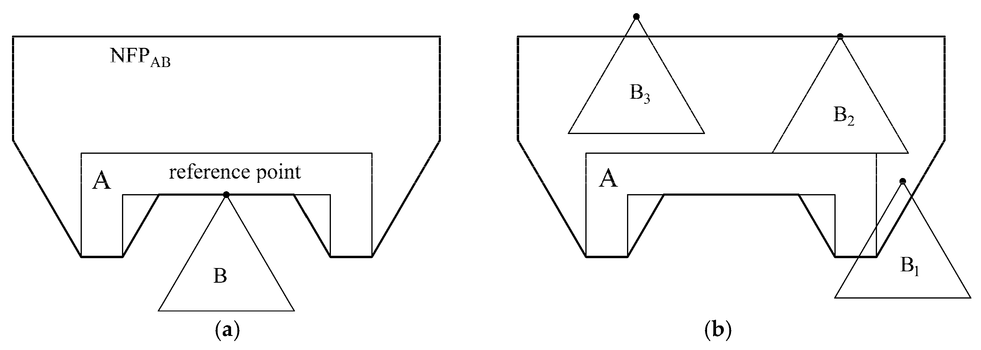
2.1. Definition and Properties

Considering that the position of polygon A is fixed, the no-fit polygon between polygons A and B is the polygon described by the locus of points, where, if the reference point of polygon B is placed, then the polygons are in contact. We denote the no-fit polygon between two polygons A and B by NFPAB. Figure 1a shows an example of a no-fit polygon. Its properties are as follows. If the reference point of B lies within the NFPAB, A overlaps B, as B1 shows in Figure 1b. If the reference point of B is on the boundary of the NFPAB, A touches B without overlap, as B2 shows in Figure 1b. If the reference point of B is outside the NFPAB, A and B are separated, as B3 shows in Figure 1b.
In conclusion, the no-fit polygon describes the region in which two polygons intersect.

2.2. Approaches for Generating NFP

Here, the main techniques that have previously been used for the creation of no-fit polygons in the literature are briefly reviewed; please see the literature [16] for more details. Note that it is easy to generate a no-fit polygon when both polygons are convex. Given two convex shapes, A and B, the no-fit polygon is generated by the following steps: (i) shape A is anticlockwise, and shape B is clockwise (see Figure 2a); (ii) all edges from A and B are translated to a single point (see Figure 2b); these edges are connected in anticlockwise order to yield the no-fit polygon (see Figure 2c).
It is very simple and extremely quick to use a standard sorting algorithm in combination with edge reordering through translation. However, no-fit polygons cannot be generated for non-convex shapes when using this method. Thus, other approaches are needed.

2.2.1. Decomposition and Phi-Function

Given the complexity of obtaining the NFP when a polygon is non-convex, one of the alternative methods is decomposition. Fast no-fit polygon creation methods can be applied if a polygon with concavities can be decomposed into convex sub-polygons. Seidal [17] suggested a fast polygon triangulation algorithm that has an O(nlogn) complexity. Watson and Tobias [18] proposed decomposing a simple polygon into a set of convex polygons by cutting between pairs of concave vertices, while Li and Milenkovic [19] decomposed a polygon into star-shaped polygons. When an irregular polygon has been decomposed into manageable shapes, the NFPs are generated by passing each sub-polygons of shape B around each sub-polygons of shape A, and finally combining the NFPs of the sub-polygons to generate the NFP of the two original polygons.
Although the decomposition method can tackle non-convex polygons, it also creates two further issues: efficient decomposition and robust recombination of the sub-NFPs. Agarwal et al. [20] conducted an extensive investigation into different decomposition and recombination operations with respect to constructing Minkowski sums of non-convex polygons. There are further challenges in the recombination operations. If edges from two sub-NFPs coincide or cross in and out of each other, careful analysis must be performed to identify whether these edges are part of the boundary of the NFP. Particular difficulty occurs if the original shapes contain holes, as it is unclear whether intersecting no-fit polygon subsections define holes or regions that can be discarded.
The Phi-function was conceived and applied by Stoyan et al. [21,22]. It is a series of mathematical expressions that represent the positional relationships of two objects. Specifically, if the value of the phi-function is greater than zero, then the objects are separated; equal to zero, then their boundaries touch; and less than zero, then they overlap, and the value should represent the Euclidean distance between the two objects. Stoyan et al. [21] analytically construct phi-functions for all primary objects (rectangles, circles and other convex polygons) and define mathematical intersection relationships for non-convex polygons through the union, intersection and complement of primary objects. Later, the authors [22] further develop phi-functions for all 2D objects that are formed by linear segments and circular arcs. This approach appears to have great potential for contributing to the field of nesting problems. However, the lack of an algorithmic process of obtaining the phi-function becomes a barrier to a wider adoption of this approach.

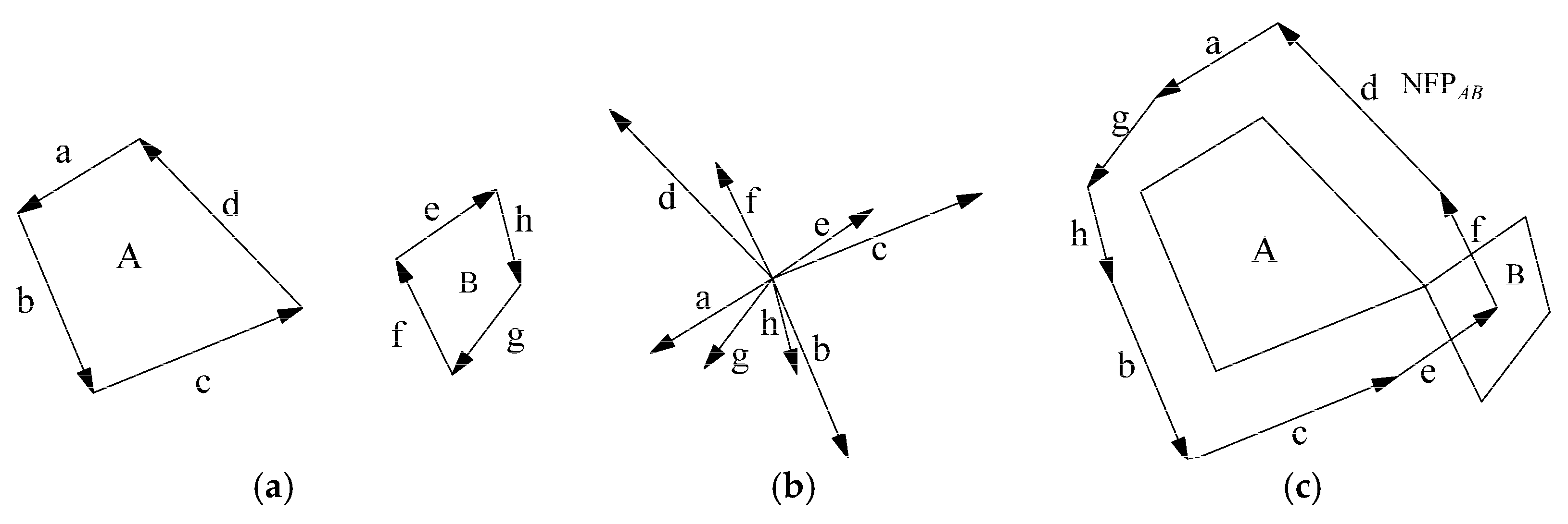
2.2.2. Minkowski Sums and Sliding Algorithm

The concept of Minkowski sums is as follows: given two arbitrary point sets, A and B, the Minkowski sum of A and B is defined by the following: AB = {a + b: aA, bB}. To produce no-fit polygons, we must use the Minkowski difference, A ⊕ −B. In addition, it requires a non-mathematical implementation of this methodology.
Ghosh developed a set of boundary addition theorems for both the convex case and non-convex case. See Ghosh [23] for a detailed explanation of these theorems. Later, Bennell et al. [24] proposed an approach that extracts key elements of Ghosh’s method and develops a set of algorithmic steps that produce the NFP. However, their approach cannot deal with internal holes, as it is difficult to detect which of the internal no-fit polygon edges can be discarded and which form the internal no-fit regions. Therefore, Bennell et al. [25] presented some modifications to provide a more robust approach. Dean [26] also presented an extension of Ghosh’s NFP algorithm.
The Minkowski sums methodology is an effective approach to produce the NFP of two polygons. However, many exceptional cases need to be considered, making this method slightly complex and hard to understand.
The first discussion and implementation of a sliding algorithm is detailed in Mahadevan’s Ph.D. thesis [27]. The key points of Mahadevan’s approach include three main steps: calculation of touching vertices and edges, determination of the translation vector and calculation of the translation length. Later, Whitwell et al. [28] proposed some improvements for Mahadevan’s approach, and the robustness of the previous algorithm was enhanced. Based on the previously published literature, we propose a more efficient and robust sliding algorithm for the generation of NFP. All known degenerate cases can be successfully addressed, and many benchmark instances are tested. In addition, inspired by the interaction of the two polygons and the definition of the no-fit polygon, Liu et al. [29] proposed a different approach for no-fit polygon calculation.

3. Improved Sliding Algorithm

The sliding algorithm derives from the definition of a no-fit polygon, which is the tracing movement. The core of this methodology is selecting the correct direction of translation according to the touching case of two polygons and then calculating the translation distance. This is an iterative procedure, and each iteration will create an edge of the no-fit polygon.

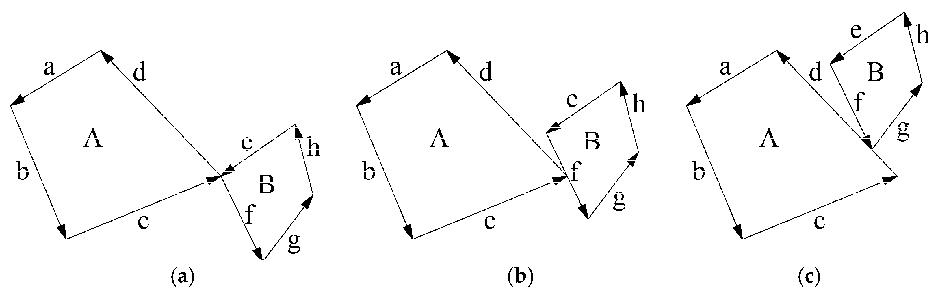
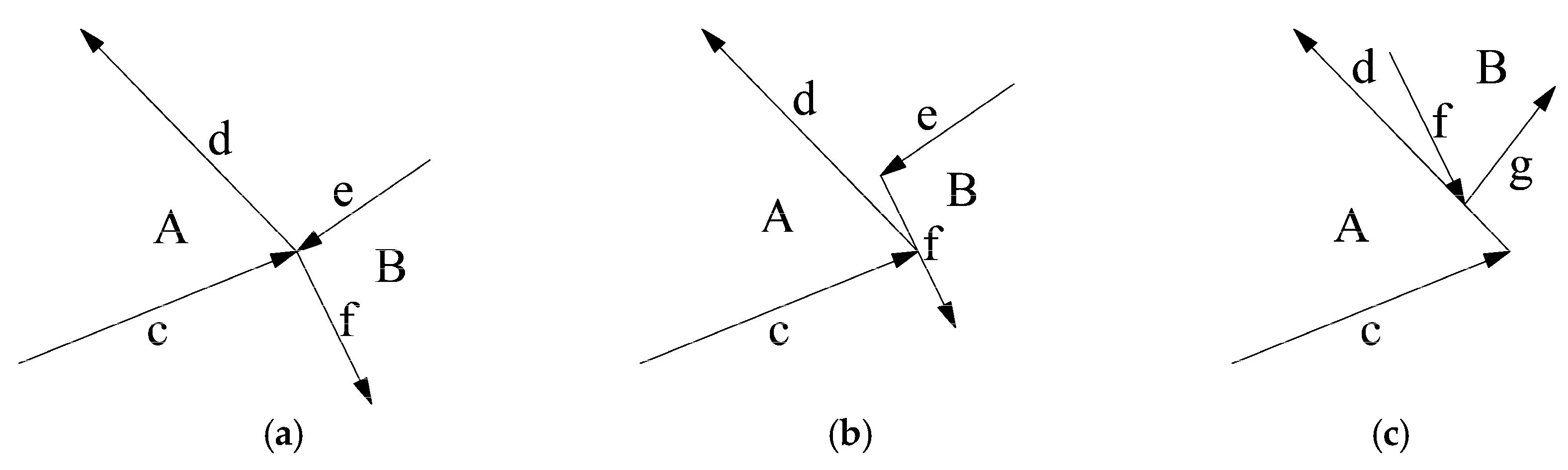
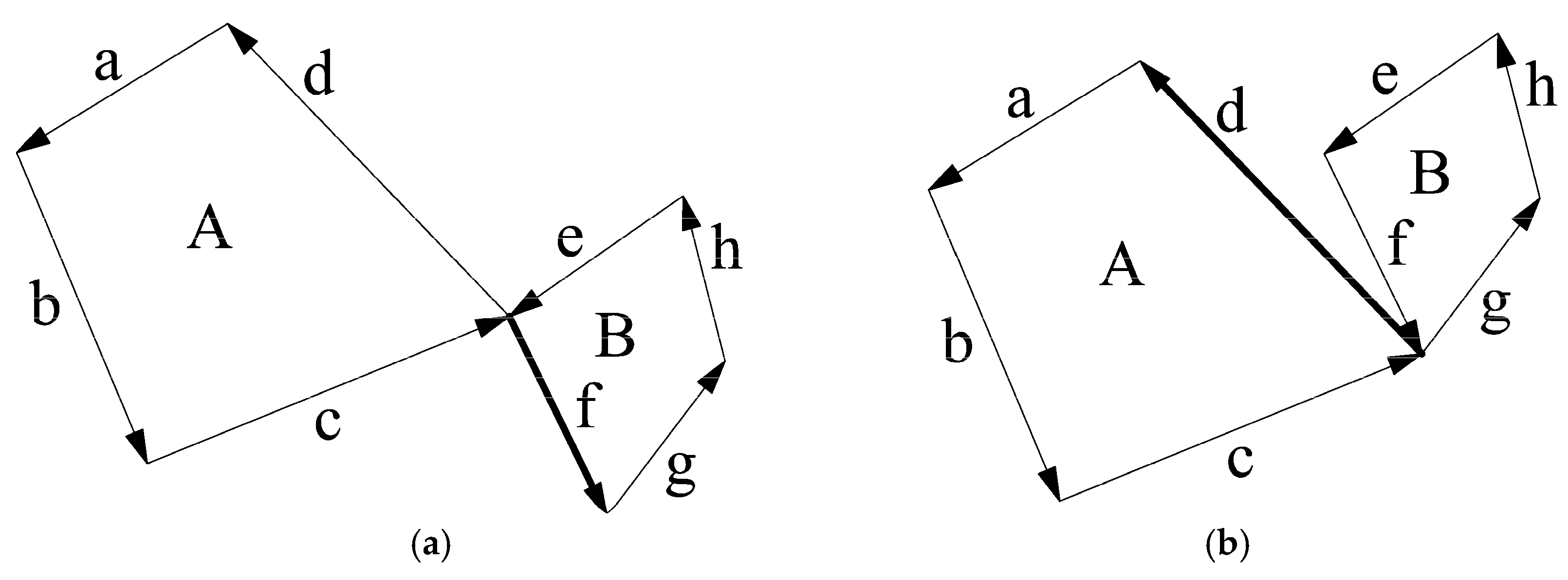
3.1. The Concept of Touching Group

In this paper, we assume that A is the fixed polygon, B is the orbital polygon and both polygons are anti-clockwise. Based on the observation, there are three possibilities of a touching case: (a) polygons A and B touch at a vertex, (b) a vertex of polygon A touches the middle of the edge of polygon B or (c) a vertex of polygon B touches the middle of the edge of polygon A. These cases are depicted in Figure 3.
Each case results in one type of touching group (see Figure 4). It consists of three or four oriented edges from polygons A and B. The adjacent edges that form the vertex of the polygon will be recorded, and the oriented edge touched in the middle by a vertex from another polygon is also recorded. Thus, the touching group has four edges (d, c, e, f), three edges (d, c, f) and three edges (f, g, d) in case (a), case (b) and case (c), respectively. It is very easy to recognize the potential translation vector for each touching group when using this concept of a touching group, resulting in simplification of the judging process compared with Whitwell’s method. For instance, we can easily identify the oriented edge d as the translation vector for polygon B in Figure 4c.

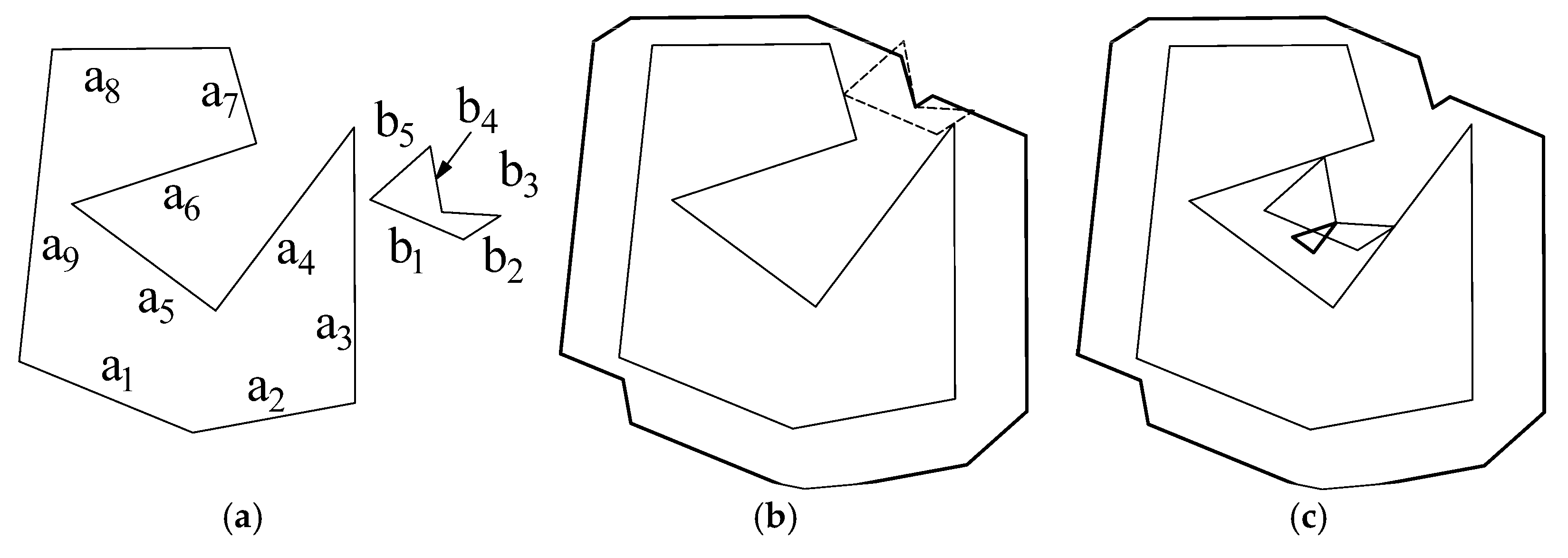
3.2. Creation of No-Fit Polygon

The process of creating NFP in the improved sliding algorithm can be broken down into the three subparts, which will be discussed in turn: finding touching groups, determining the translation vector from all touching groups and computing the translation distance.

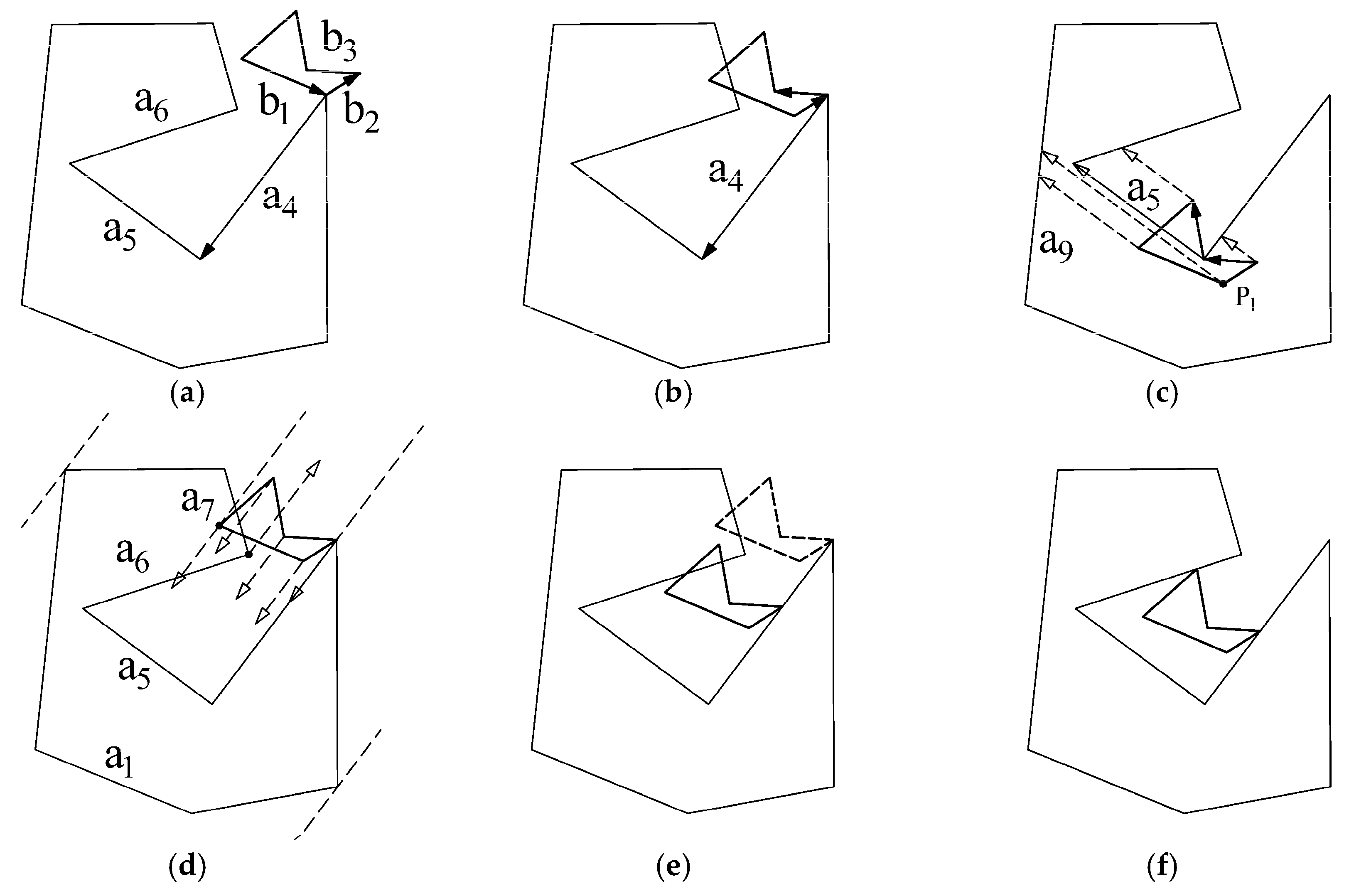
3.2.1. Find the Touching Group

The creation of a no-fit polygon starts with the operation of finding the touching group between two polygons. The ability to correctly find touching edges is vital to the sliding approach because the remaining two subparts are based on this. This is achieved by testing each edge of fixed polygon A against each edge of orbital polygon B. Note that it only needs to test whether the starting point of the edge touches the starting point or the middle of the edge from another polygon. For example, in Figure 3a, the starting point of edge d touches the starting point of edge f. In Figure 3b, the starting point of edge d touches in the middle of edge f. The touching groups found in this step will be stored in a list, referred to here as the T list.

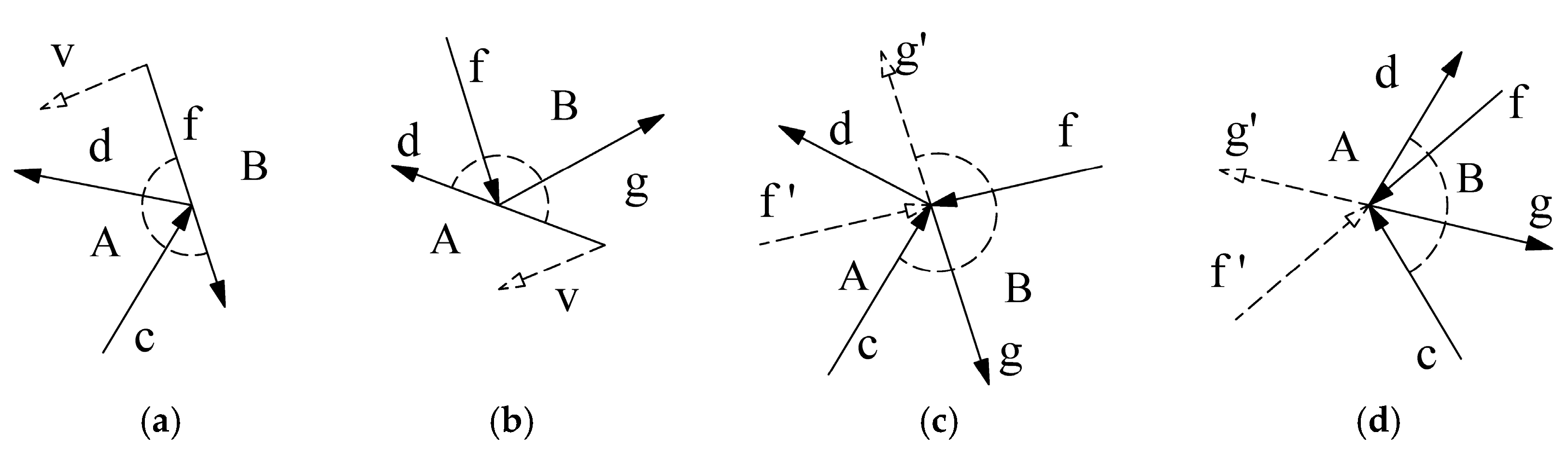
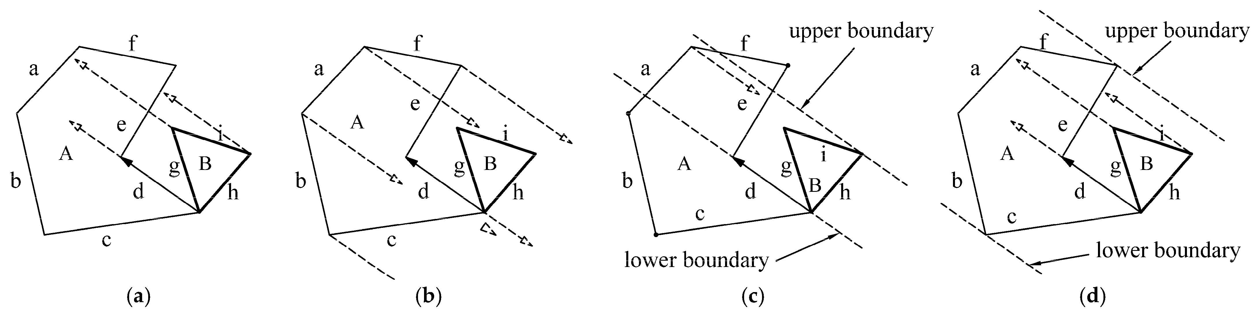
3.2.2. Determine Translation Vector

(i)
Recognize the potential translation vector
The first step is to recognize the potential translation vector from each touching group in the T list. For the first type of touching group, as shown in Figure 4a, only the edge pair in which the starting point coincides is considered. If the ending point of edge f from the orbital polygon is on the left side of another edge d from the fixed polygon, edge f is the potential translation vector. Otherwise, edge d is the potential translation vector. As shown in Figure 5a, the ending point of edge f is on the left side of edge d, so the potential translation vector is edge f. As shown in Figure 5b, the potential translation vector is edge d because the ending point of edge g is on the right side of edge d or these two edges are parallel. Note that the oriented edge needs to be reversed if it derives from the orbital polygon. For example, edge f should reverse in Figure 5a. For the second and third types of touching groups, the potential translation vector is the edge where the vertex touches (see Figure 4b,c, edges f and d).
(ii)
Determine the feasible translation vector
Each touching group in the T list produces a potential translation vector, but not all of them are feasible. In other words, the orbital polygon translating along the vector may intersect with the fixed polygon. For instance, assuming that the touching case of two polygons is as shown in Figure 6, there are two touching groups, and we can identify that the potential translation vectors are edges e and d. If we translate polygon B along vector d, this would result in an intersection between edges i and e or g and e. Thus, vector d is infeasible, while vector e is feasible.
Hence, we propose a test to determine whether the potential translation vector is feasible. First, we calculate the angular direction at the touch point for which the edge of the orbital polygon can move without intersecting with the edge of the fixed polygon. Then, we identify whether the potential translation vector from other touching groups is within the angular direction. Note that a potential translation vector is feasible only if it is within the angular direction of all other touching groups. Based on the observation, the feasibility test only considers four types, as shown in Figure 7.
For the second and third types of touching groups shown in Figure 7a,b, the angular direction (given by the circular arcs) is easy to calculate, and we only need to test the potential translation vector v on the right side of (or parallel to) the potential translation vector produced by this touching group. Obviously, the vector v is feasible for this touching group, as shown in Figure 7a, and not for the touching group, as shown in Figure 7b.
For the first type of touching group, i.e., touching at a vertex, it needs to determine the boundaries before calculating the angular direction. As shown in Figure 7c, if edge g′ (produced by reversing edge g) is on the right side of edge d, the boundary is g′. Otherwise, the boundary is edge d. In the same way, we can recognize that the second boundary is edge c. Thus, the angular direction is produced by edges c and g′. In Figure 7d, the boundary edges are edges a1 and a2. Note that the potential translation vector is feasible for this touching group if it is on the right side of (or parallel to) one of the boundary edges for the case of Figure 7c, while it is feasible for this touching group only if it is on the right side of both boundary edges for the case of Figure 7d.
(iii)
Select a feasible translation vector
According to the observation, there is only one feasible translation vector in most cases in the process of creating a no-fit polygon. However, when degenerate cases such as holes, interlocking concavities and jigsaw-type pieces occur, many feasible translation vectors exist. A good method is needed to select a vector for producing the correct NFP. The method chooses the edge that is nearest (in edge order of fixed polygon) to the previous move. As shown in Figure 8b, the edge order of the previous move is 2 in this situation, and the nearest translation vector is edge a3, so the orbital polygon translates along the vector a3.
In conclusion, there are three subparts of this step: finding the potential translation vector from the touching group, judging whether it is feasible and selecting a suitable vector if there are more than one. The Pseudo code of this step is shown in Algorithm 1.
Algorithm 1: Determine Translation Vector.
Input: T list // T list,;
Input: t1; // last touching group;
Output: t2; // the selected touching group
t = the number of touching groups in T;
for each touching group in T do
Get the potential translation vector of Ti;
Calculate angular direction of Ti;
end for
if t is equal to 1
t2 = T0;
return;
i = 0;
for i < t do
for j < t do
if j is not equal to i
// do feasible test
Get the potential vector vi in Ti;
if vi is not suitable for Tj
Flag vi is infeasible;
break;
j = j + 1;
end for
i = i + 1;
end for
if only one feasible translation vector in T
t2 = feasible translation vector in T;
return;
t2 = Select a feasible vector from T based on t1;
return;

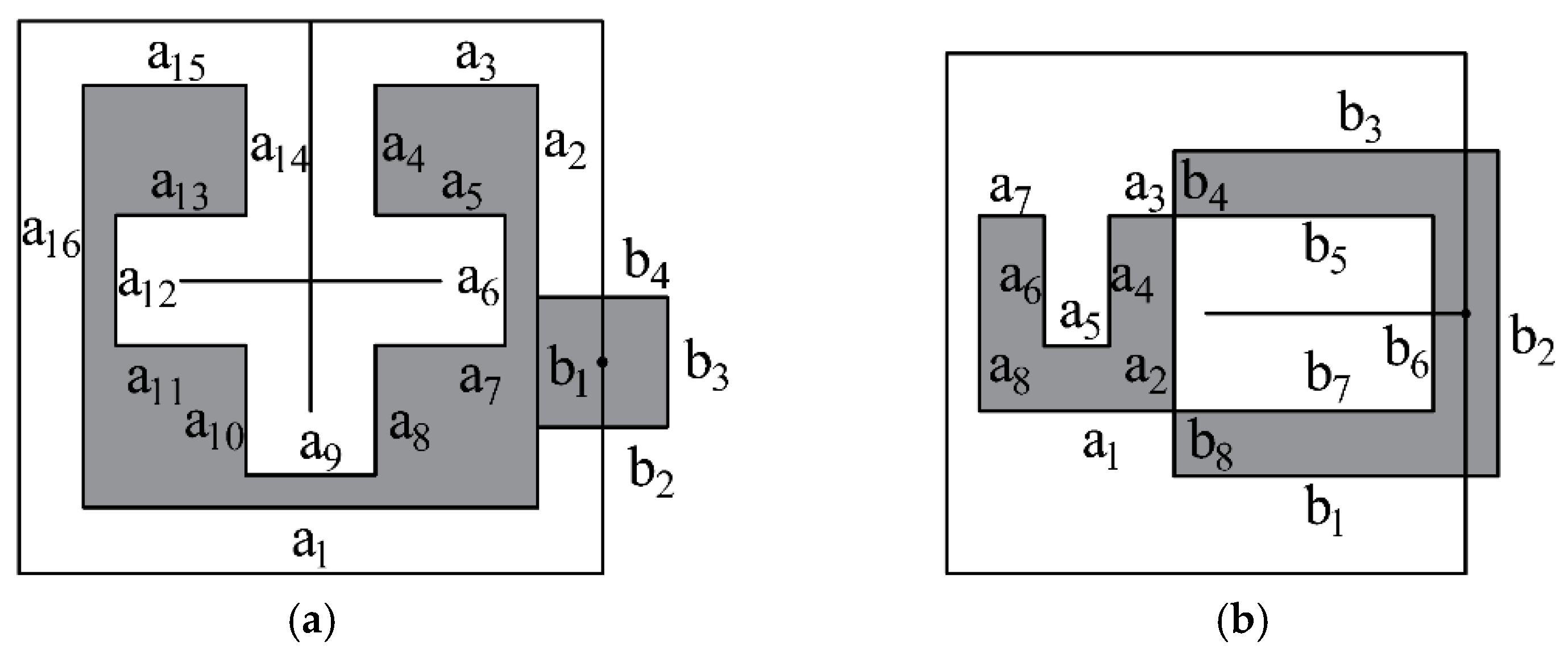
3.2.3. Compute Translation Distance

The translation vector only provides the direction of movement of the orbital polygon because the translation distance is not always the full length of the vector from the touching group. As shown in Figure 9a, when polygons A and B touch at a vertex, there is only one touching group, and the translation vector is oriented edge d. Polygon B will intersect with polygon A if applying the entire translation vector d, as shown in Figure 9b. Therefore, we compute the feasible translation distance to avoid overlap. The task is trivial to the human eye. The maximal translation distance is the vector v, as shown in Figure 9c. However, for the computer, there needs to be a set of algorithmic steps.
(i)
Computation method
The method projects the translation vector at each of the vertices of polygon B and tests it for intersection with all edges of polygon A, as shown in Figure 10a. The projection is also executed in the opposite direction for the vertices of polygon A, as shown in Figure 10b. Once the vertex of polygon B that will cross into polygon A is found and the length of the new translation vector is smaller than the current translation vector, the current translation vector is replaced by the new one. This method ensures that the correct non-intersecting translation is found.
(ii)
Acceleration strategy
This is the most time-consuming operation for the sliding algorithm, and the time complexity is O(mn) in theory, where m and n are the numbers of vertices of polygons A and B, respectively. This paper proposes a point exclusion strategy to accelerate this operation. The strategy identifies the vertex that will not cross into the polygon when translating along the selected vector, and then does not test these vertices. It can take less time than we thought if many ineffective tests are excluded.
First, we calculate the upper boundary and lower boundary of the fixed polygon and orbital polygon based on the translation vector. Then, a simple test for the vertex of the polygon is performed before testing it for intersection with all edges of another polygon. Specifically, if the vertex is out of the range of the boundary, there is no need to test it for intersection with other polygon edges. Figure 10c,d show in detail an example of this strategy. In Figure 10c, three vertices of polygon A are out of the range of the boundary, and the two endpoints of edge d can also be excluded. Theoretically, the operation of projecting and intersection test needs to be executed 6 × 3 times, while practically, it only needs 1 × 3 times by using the point exclusion strategy. The effect of reducing the computation time is significant and will be further verified in Section 4. The Pseudo code of this step is shown in Algorithm 2.
Up to now, the direction and distance of translation have been determined, and the final step is to translate polygon B by the shortened translation vector. Then, we perform a test to detect if the reference point of polygon B has returned to its initial starting position. If not, the process of creating a no-fit polygon is restarted from the finding touching group.
Algorithm 2: Compute translation distance.
Input: PA, PB //two polygons; t2 // the selected touching group
Get the translation vector v in t2;
Initialize ub, lb; // the upper and lower bound
Get the boundary ub and lb about PA based on v;
i = 0;
for each vertex point p a of PA do
if p a is not in ub and lb bound
continue; // point exclusion test
for each edge e of PB do
Calculate the cross point p c of the p a along v with edge e;
if p c exists // intersection happened
Get distance d between p c and p a ;
if d less than the current length of v;
The starting point of v = p c ;
The ending point of v = p a ;
end for
end for
Get the boundary ub and lb about PB based on v;
i = 0;
for each vertex point p b of PB do
if p b is not in ub and lb bound do
continue; // point exclusion test
for each edge e of PA do
Calculate the cross point p c of the p b along v with edge e;;
if p c exists // intersection happened
Get distance d between p c and p b ;
if d less than the current length of v;
The starting point of v = p b ;The ending point of v = p c ;
end for
end for

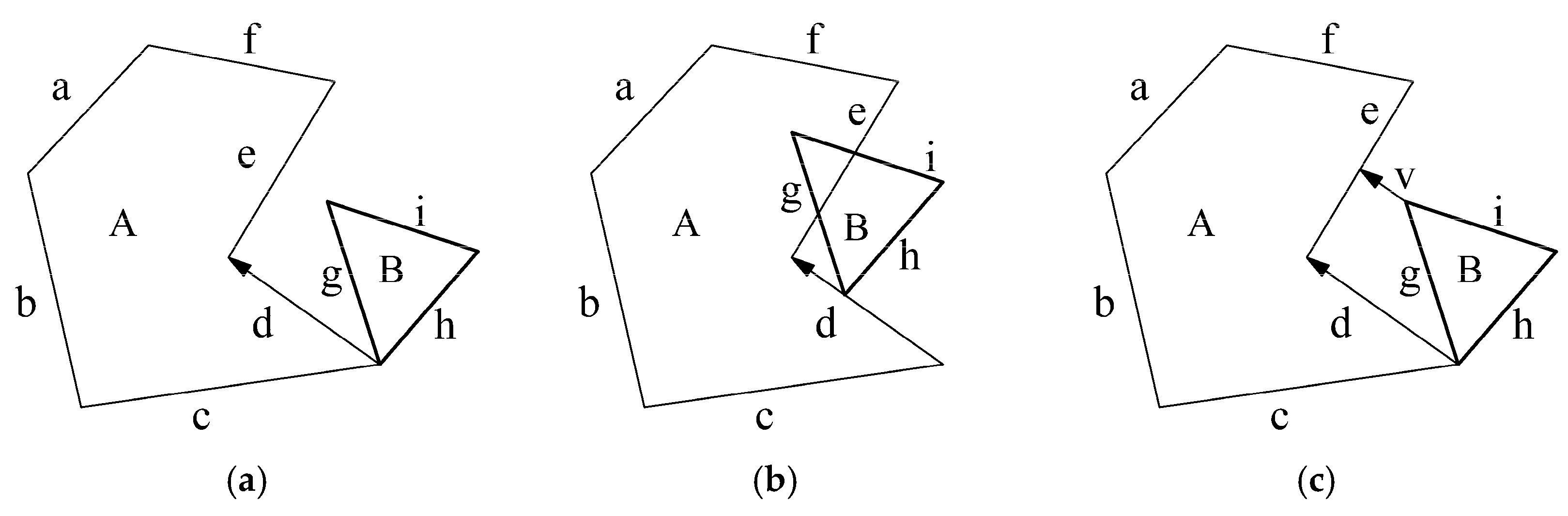
3.3. Searching Oher Start Positions

The creation of NFP in the sliding algorithm starts with selecting a touching but non-intersecting position for two polygons. This is an easy task, and usually, the largest y-coordinate of orbital polygon B is placed touching the smallest y-coordinate of fixed polygon A. Then, the three steps described in Section 3.1 are iteratively performed to create the no-fit polygon. An example is shown in Figure 11b. However, the produced no-fit polygon may be incomplete if only these steps are performed. As shown in Figure 11b, polygon A has concavity, and its entrance is so narrow that polygon B is not able to slide into the concavity. Thus, another method is needed to determine this possibility.

3.3.1. Method of Searching Feasible Starting Position

If the position of orbital polygon B shown in Figure 11c can be found, then the creation of a no-fit polygon can start with this position. Whitwell et al. [28] proposed an approach to identify such possibilities. The basic principle is that if an edge of a fixed polygon has not been traversed when creating a no-fit polygon, then these edges will be searched for feasible start positions. Specifically, given an edge u of fixed polygon A, the first step is to translate polygon B such that the first vertex of it is aligned to the start point of u; then, performing an overlap test [30], if the polygons do not intersect in this position then this is a feasible start position; if they intersect, then performing a sliding operation including calculating the translation distance and translating polygon B along edge u, this operation is similar to the steps described in Section 3.2.3. After sliding, the overlap test is executed again. This is an iterative process until a non-intersecting position is found or the end of edge u is reached. If the first vertex of polygon B cannot find a feasible starting point, then try the rest of its vertices. Note that the edge of the fixed polygon is flagged as “visited” whether the feasible start position is found or not. The Pseudo code of searching for other starting points is shown in Algorithm 3.
Algorithm 3: Search other Start Point.
Input: PA, PB //two polygons,
Input: Ptnfp; // the starting point of new NFP
Initialize V = ; // the list of storing all translation vectors
for each edge e n of PA do
if e n is visited do
continue;
Set   e n is visited;
for each edge e m of PA
Move P B by making starting point of e n and e m coincidence;
if both e m 1 and e m are not on the right side of e n  do
continue; // “right sidetest
V = ; // clear stored vectors
If the result of getting translation vectors ( P A ,   P B ,   e n ) is false do
continue; // Algorithm 4
while the starting point of e m does not on the ending point of e n  do
if PA does not overlap with PB at this position
Ptnfp = PBrf; // the reference point PBrf of PB
return true;
Shorten all vectors in V and get the translation vector v;
Translate PB by vector v;
end while
end for
end for
return false;

3.3.2. Acceleration Strategies

The method can fully search for feasible starting positions, but it is time-consuming due to three main aspects. First, for an unvisited edge of a fixed polygon, all vertices of the orbital polygon need to be tested. Second, the test contains the operation of computing translation distance, which takes a lot of time in the sliding algorithm. Third, the overlap test is also time-consuming and must be performed after each translation. Hence, some strategies are applied to improve the efficiency of this method.
The first acceleration strategy is to examine whether the two connected edges of polygon B are both on the right of or parallel to edge u of polygon A [28], called the “right side” test. The D-function [31] is used to recognize the relative position of a point with respect to an oriented edge. If either of the edges are left of u, then overlapping between polygons A and B occur and never yield a feasible starting position when sliding along vector u. Hence, we can abandon this vertex and test the next one, which results in reducing the number of operations of computing translation distance and overlap test, thereby improving efficiency. Figure 12a,b show examples of this strategy. In Figure 12a, edge b2 is on the left side of edge a4, which dissatisfies the requirement. However, in Figure 12b, both edges b2 and b3 are on the right side of edge a4.
The second strategy is a “point inclusion”. In the operation of computing the translation distance, if the minimal distance corresponding to a certain vertex of polygon B is larger than or equal to the length of edge u and this vertex is inside of polygon A, then this vertex of polygon B is abandoned because the two polygons always overlap when sliding along edge u. This is the same for the vertex of polygon A. As shown in Figure 12c, when projecting translation vector a5 at vertex P1 and only intersecting with a9, the translation distance is obviously larger than the length of a5 and P1 is inside polygon A, so the vertex can be abandoned, and there is no need to take a sliding operation.
The third acceleration strategy is the improved “point exclusion” strategy. The improvement is keeping all translation vectors in the operation of computing translation distance instead of adopting a replacement strategy. This method avoids recalculating after translating polygon B and only needs to shorten all stored vectors. See an example shown in Figure 12d. There is only one vertex of polygon A (the starting point of a7) that needs to be calculated when applying the point exclusion strategy. This vertex will intersect with edges b1 and b4, resulting in two translation vectors being stored. After iteratively performing the overlap test and sliding operation, the feasible start position is found, as shown in Figure 12f. The Pseudo code of the improved operation of computing the translation distance is shown in Algorithm 4.
Algorithm 4: Get translation vectors.
Input: PA, PB; // two polygons
Input: v; // the oriented edge of PA
Output: V; //the list of storing all vectors
Initialize ub, lb; // the upper and lower bound
Initialize Vt = ; // temporarily store the translation vectors
Get the boundary ub and lb about PA based on v;
for each vertex point p a of PA do
if p a is not in ub and lb bound do
continue; // point exclusion test
for each edge e of PB do
Calculate the cross point p c of the p a along v with edge e;;
if p c exists do
Add new vector u = p a p c to Vt;
end for
if Vt is not empty do
if does not pass the point inclusion test do
return false;
else
Add all vectors in Vt to V;
Vt = ;
end for
Get the boundary ub and lb about PB based on v;
for each vertex point p b of PB do
if p b is not in ub and lb bound do
continue; // point exclusion test
for each edge e of PA do
Calculate the cross point p c of the p b along v with edge e;
if p c exists
Add new vector u = p c p a to Vt;
end for
if Vt is not empty do
if does not pass the point inclusion test do
return false;
else
Add all vectors in Vt to V;
Vt = ;
end for
return true;

3.3.3. The ISA Algorithm

According to the detailed description of our proposed algorithm in Section 3.1, Section 3.2 and Section 3.3.1, the Pseudo code of the ISA algorithm is described by Algorithm 5.
Algorithm 5: Sliding Algorithm.
Input: PA, PB //two polygons
Initialize T = ; //T list for storing touching groups
Initialize two touching groups t1, t2;
Initialize creation = true; NFPs = ;
PtA(ymin) = the point of minimum y-coordinate of PA;
PtB(ymax) = the point of maximum y-coordinate of PB;
Move PB to make PtB(ymax) touch the PtA(ymin);
Ptnfp = the reference point PBrf of PB; //the starting point of NFP
while the creation is true do
Clear the T list;
Find touching groups (PA, PB, T);
// Algorithm 1
Determine translation vector (T, t1, t2);
// Algorithm 2
Compute translation distance (PA, PB, t2);
Flag the edge of PA in T2 is visited;
t1 = t2;
Initialize a new edge e1;
The starting point of e1 = PBrf;
Move PB using the translation vector stored in t2.
The ending point of e1 = PBrf;
Produce new edge e1 of the no-fit polygon nfp;
if Ptnfp is equal to PBrf //Get an NFP
Add the current no-fit polygon nfp to NFPs;
bool over = false;
while over is false do
if search other start point (PA, PB, Ptnfp) //Algorithm 3
// Feasible start position may be the vertex of
// created NFP in rare cases
if the starting point is the vertexes of NFPs
  continue;
if (the position of PA and PB is Jigsaw case)
Add the current no-fit polygon nfp to NFPs;
continue;
over = true; //Find a feasible start point.
else
creation = false;
over = true;
end while
end if
end while
return NFPs;

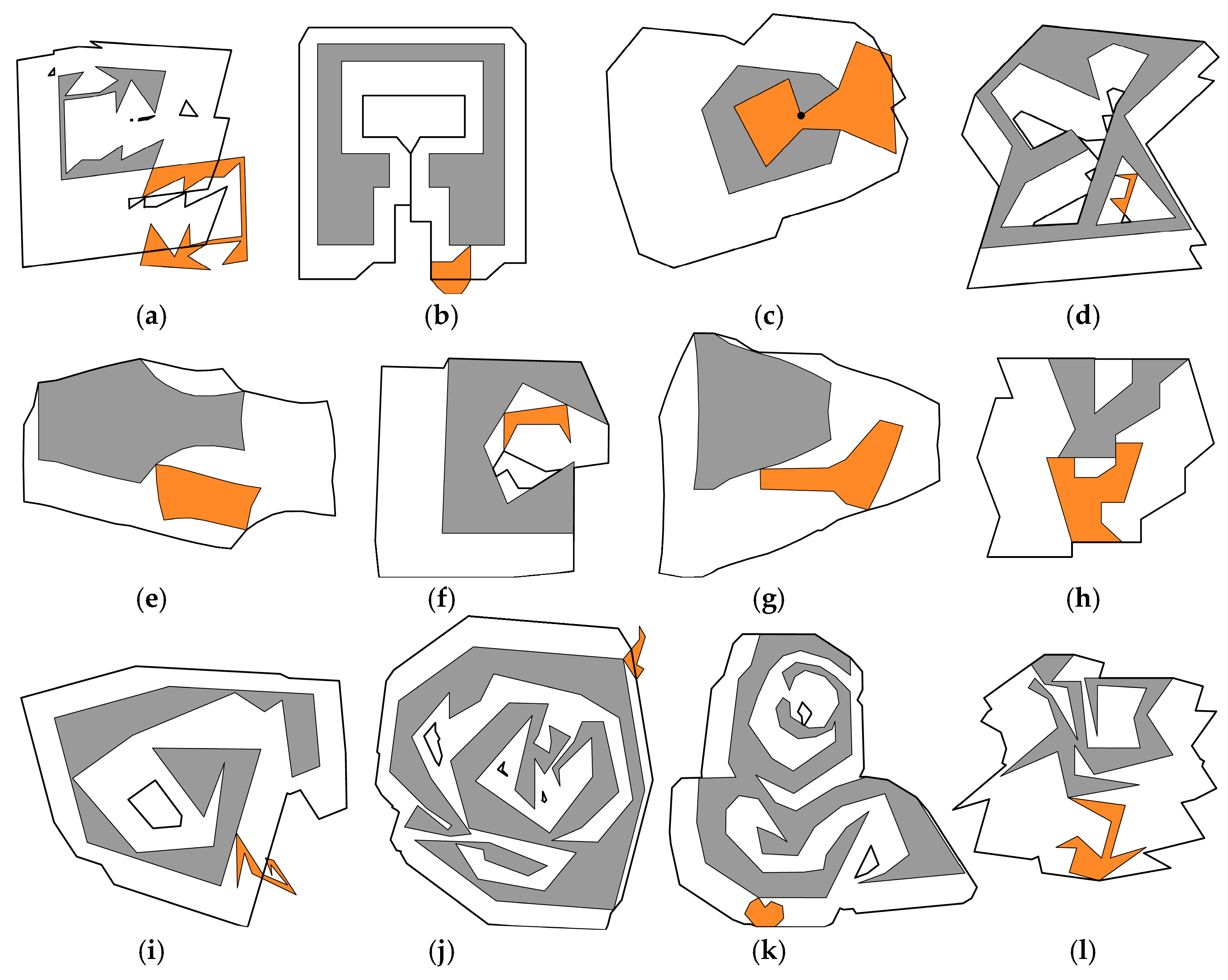
4. Computational Experiments

To evaluate the robustness of the improved sliding algorithm, many special and complex instances provided by published literature [24,25,28] are used to test the ISA. These instances involve characteristics such as a large number of edges, interlocking positions, exact sliding, jigsaw-type fits and concavities, and the results are shown in Figure 13.
To further test the robustness and efficiency of ISA, we also use it to generate the NFP for all polygons from the benchmark datasets. Each dataset contains many simple polygons and is used as a common test set in the cutting and packing community. The computation times for benchmark datasets are provided in Table 1. The procedure of the proposed algorithm was coded in Visual Studio C++, and the instances were run on a PC with 8 GB, Core i7 1.8 GHz processer.

4.1. Robustness Performance of ISA

It is difficult to create no-fit polygons involving holes. However, the no-fit polygon can be generated easily and completely using the operation of searching other start positions. In Figure 13, the no-fit polygon contains holes for Figure 13a,d,f,i–k; in particular, there are multiple holes for a, d, j and k. Furthermore, the fixed polygon has concavities within the concavities in Figure 13j,k. There also exist cases involving sliding through exactly fitting ‘‘passageways’’ that are hard to handle. Figure 13b shows such a case, and another example of this case is previously discussed in Figure 8.
Figure 13c shows the problem case involving jigsaw pieces that fit together with no movement. Thus, the no-fit polygon is a singular feasible point rather than an internal loop. After obtaining a feasible start position, our algorithm will perform a simple test to determine whether there is a feasible translation vector to identify this case. Most of the previous approaches including the Minkowski sun and convex decomposition, have difficulty handling this case [28]. The no-fit polygons shown in Figure 13e,g are from the “Swim” benchmark datasets.

4.2. Efficiency Performance of ISA

Table 1 shows the creation times for benchmark datasets by the improved sliding algorithm (ISA). To evaluate the effect of the point exclusion strategy (PES) and the point inclusion test (PIT) on the algorithm’s efficiency, we also test the creation time of the no-fit polygon for the ISA without the PES and PIT. The meaning of the capital letters in the header of Table 1 is illustrated by notes below the table. The column of “In.” represents the percent of increased time when compared to the ISA.
All experiments evaluating the performance of Whitwell’s approach were conducted on a Pentium 42 GHz processor with 256 MB RAM. The experimental results in Table 1 show that the ISA creates no-fit polygons quicker than Whitwell’s approach for all of the datasets, especially for the poly5b, poly4b, Jakobs1, Jakobs2 and swim datasets. Although this comparison is unfair due to the difference in hardware, it shows that the method proposed in this paper is able to quickly generate no-fit polygons and that all the improvements contribute to the computing efficiency. The strategy of PIT is effective in terms of improving efficiency for many datasets, especially for the swim dataset, for which the average number of edges is larger than others. However, there is a possibility that the creation time will increase because it takes time to perform the test.
Computational results show that the proposed PES can largely increase computational efficiency, and the more edges the polygon has, the better. This is further verified by the instance named Arc1, in which all edges of the polygons are arcs. The results are shown in Table 2. The arcs are discretized with different precisions, resulting in different numbers of edges. The creation time is reduced by 20 percent when the average number of edges is 76.0. It is able to be reduced by 51.2 percent when the average number of edges is 652.0.

5. Conclusions and Future Works

In this paper, an efficient and robust sliding algorithm for generating a no-fit polygon is proposed. Creating a no-fit polygon only contains three steps based on the proposed concept of touching group, i.e., finding the touching group, determining the translation vector and computing the translation distance. The first feasible start position is easy to identify, but other starting positions are likely to exist when the polygon is non-convex. Hence, the searching other start positions procedure is adopted to produce a complete no-fit polygons. Many strategies are proposed to improve the algorithm’s efficiency. Experimental results show that the algorithm is highly efficient for the creation of a no-fit polygon. The calculation time in benchmark instances is increased by 21.0% and 3.20% on average if there is no PES and PIT, respectively. The proposed algorithm is a computational geometric algorithm used for generating no-fit polygons of 2D graphics. It cannot handle curves, so the discretization operation is needed. In other words, the input graphic is a simple polygon without self-intersecting edges. To the best of our knowledge, the algorithm has many applications, such as irregular packing problems, engineering and robot motion planning and the aircraft parking stand allocation problem.
Future works need to further investigate how to reduce the time of the second phase, i.e., searching other feasible start positions to generate a complete NFP, and propose strategies to further improve the efficiency.

Author Contributions

Q.L.: conceptualization, methodology, validation, formal analysis, writing—original draft, writing—review and editing; Y.R.: supervision, project administration, writing—review and editing, funding. All authors have read and agreed to the published version of the manuscript.

Funding

This research is funded by the National Natural Science Foundation of China (Grant no. 51975231) and Fundamental Research Funds for the Central Universities (Grant no. 2019kfyXKJC043).

Institutional Review Board Statement

Not applicable.

Informed Consent Statement

Not applicable.

Data Availability Statement

Not applicable.

Acknowledgments

The authors would like to thank the referees for their constructive comments that improved the presentation as well as the content of the paper.

Conflicts of Interest

The authors declare that they have no known competing financial interests or personal relationships that could have appeared to influence the work reported in this paper.

References

  1. Elkeran, A. A new approach for sheet nesting problem using guided cuckoo search and pairwise clustering. Eur. J. Oper. Res. 2013, 231, 757–769. [Google Scholar] [CrossRef]
  2. Rao, Y.; Wang, P.; Luo, Q. Hybridizing beam search with tabu search for the irregular packing problem. Math. Probl. Eng. 2021, 2021, 5054916. [Google Scholar] [CrossRef]
  3. Alves, C.; Brás, P.; de Carvalho, J.V.; Pinto, T. New constructive algorithms for leather nesting in the automotive industry. Comput. Oper. Res. 2012, 39, 1487–1505. [Google Scholar] [CrossRef]
  4. Hu, X.; Li, J.; Cui, J. Greedy adaptive search: A new approach for large-scale irregular packing problems in the fabric industry. IEEE Access 2020, 8, 91476–91487. [Google Scholar] [CrossRef]
  5. Labrada-Nueva, Y.; Cruz-Rosales, M.H.; Rendón-Mancha, J.M.; Rivera-López, R.; Eraña-Díaz, M.L.; Cruz-Chávez, M.A. Overlap detection in 2D amorphous shapes for paper optimization in digital printing presses. Mathematics 2021, 9, 1033. [Google Scholar] [CrossRef]
  6. Luo, Q.; Rao, Y.; Peng, D. GA and GWO algorithm for the special bin packing problem encountered in field of aircraft arrangement. Appl. Soft Comput. 2022, 114, 108060. [Google Scholar] [CrossRef]
  7. Gonçalves, J.F.; Wäscher, G. A MIP model and a biased random-key genetic algorithm based approach for a two-dimensional cutting problem with defects. Eur. J. Oper. Res. 2020, 286, 867–882. [Google Scholar] [CrossRef]
  8. Chen, K.; Zhuang, J.; Zhong, S.; Zheng, S. Optimization Method for Guillotine Packing of Rectangular Items within an Irregular and Defective Slate. Mathematics 2020, 8, 1914. [Google Scholar] [CrossRef]
  9. Romanova, T.; Pankratov, O.; Litvinchev, I.; Stetsyuk, P.; Lykhovyd, O.; Marmolejo-Saucedo, J.A.; Vasant, P. Balanced Circular Packing Problems with Distance Constraints. Computation 2022, 10, 113. [Google Scholar] [CrossRef]
  10. Qin, Y.; Chan, F.T.S.; Chung, S.H.; Qu, T.; Niu, B. Aircraft parking stand allocation problem with safety consideration for independent hangar maintenance service providers. Comput. Oper. Res. 2018, 91, 225–236. [Google Scholar] [CrossRef]
  11. Martinez-Sykora, A.; Alvarez-Valdes, R.; Bennell, J.; Ruiz, R.; Tamarit, J. Matheuristics for the irregular bin packing problem with free rotations. Eur. J. Oper. Res. 2017, 258, 440–455. [Google Scholar] [CrossRef]
  12. Júnior, B.A.; Pinheiro, P.R.; Coelho, P.V. A parallel biased random-key genetic algorithm with multiple populations applied to irregular strip packing problems. Math. Probl. Eng. 2017, 2017, 1670709. [Google Scholar]
  13. Pinheiro, P.R.; Amaro, B., Jr.; Saraiva, R.D. A random-key genetic algorithm for solving the nesting problem. Int. J. Comput. Integr. Manuf. 2016, 29, 1159–1165. [Google Scholar] [CrossRef]
  14. Cherri, L.H.; Mundim, L.R.; Andretta, M.; Toledo, F.M.; Oliveira, J.F.; Carravilla, M.A. Robust mixed-integer linear programming models for the irregular strip packing problem. Eur. J. Oper. Res. 2016, 253, 570–583. [Google Scholar] [CrossRef]
  15. Costa, M.T.; Gomes, A.M.; Oliveira, J.F. Heuristic approaches to large-scale periodic packing of irregular shapes on a rectangular sheet. Eur. J. Oper. Res. 2009, 192, 29–40. [Google Scholar] [CrossRef]
  16. Bennell, J.A.; Oliveira, J.F. The geometry of nesting problems: A tutorial. Eur. J. Oper. Res. 2008, 184, 397–415. [Google Scholar] [CrossRef]
  17. Seidel, R. A simple and fast incremental randomized algorithm for computing trapezoidal decompositions and for triangulating polygons. Comput. Geom. Theory Appl. 1991, 1, 51–64. [Google Scholar] [CrossRef]
  18. Watson, P.D.; Tobias, A.M. An Efficient Algorithm for the Regular W 1 Packing of Polygons in the Infinite Plane. J. Oper. Res. Soc. 1999, 50, 1054. [Google Scholar] [CrossRef]
  19. Li, Z.; Milenkovic, V. Compaction and separation algorithms for non-convex polygons and their applications. Eur. J. Oper. Res. 1995, 84, 539–561. [Google Scholar] [CrossRef]
  20. Agarwal, P.K.; Flato, E.; Halperin, D. Polygon decomposition for efficient construction of Minkowski sums. Comput. Geom. 2002, 21, 39–61. [Google Scholar] [CrossRef]
  21. Stoyan, Y.; Scheithauer, G.; Gil, N.; Romanova, T. Φ-functions for complex 2D-objects. Q. J. Belg. Fr. Ital. Oper. Res. Soc. 2004, 2, 69–84. [Google Scholar]
  22. Chernov, N.; Stoyan, Y.; Romanova, T.; Pankratov, A. Phi-Functions for 2D Objects Formed by Line Segments and Circular Arcs. Adv. Oper. Res. 2012, 2012, 346358. [Google Scholar] [CrossRef] [PubMed]
  23. Ghosh, P.K. An algebra of polygons through the notion of negative shapes. CVGIP Image Underst. 1991, 54, 119–144. [Google Scholar] [CrossRef]
  24. Bennell, J.; Dowsland, K.; Dowsland, W. The irregular cutting-stock problem—A new procedure for deriving the no-fit polygon. Comput. Oper. Res. 2001, 28, 271–287. [Google Scholar] [CrossRef]
  25. Bennell, J. A comprehensive and robust procedure for obtaining the nofit polygon using Minkowski sums. Comput. OR 2008, 35, 267–281. [Google Scholar] [CrossRef]
  26. Dean, H.T.; Tu, Y.; Raffensperger, J.F. An improved method for calculating the no-fit polygon. Comput. Oper. Res. 2006, 33, 1521–1539. [Google Scholar] [CrossRef]
  27. Mahadevan, A. Optimisation in Computer Aided Pattern Packing. Ph.D. Thesis, North Carolina State University, Raleigh, NC, USA, 1984. [Google Scholar]
  28. Burke, E.; Hellier, R.; Kendall, G.; Whitwell, G. Complete and robust no-fit polygon generation for the irregular stock cutting problem. Eur. J. Oper. Res. 2007, 179, 27–49. [Google Scholar] [CrossRef]
  29. Huyao, L.; Yuanjun, H.; Bennell, A.J. The irregular nesting problem: A new approach for nofit polygon calculation. J. Oper. Res. Soc. 2007, 58, 1235–1245. [Google Scholar] [CrossRef]
  30. Ferreira, J.C.; Alves, J.C.; Albuquerque, C.; Oliveira, J.F.; Ferreira, J.S.; Matos, J.S. A flexible custom computing machine for nesting problems. In Proceedings of the XIII DCIS, Madrid, Spain, 17 November 1998; pp. 348–354. [Google Scholar]
  31. Konopasek, M. Mathematical treatments of some apparel marking and cutting problems. US Dep. Commer. Rep. 1981, 99, 90857-10. [Google Scholar]
Figure 1. (a) Polygons A, B and construction of NFPAB and (b) The properties of the no-fit polygon.
Mathematics 10 02941 g001
Figure 2. Method of generating a no-fit polygon with convex polygons. (a) Polygons A and B; (b) All edges are moved to a single point; (c) Generation of NFPAB.
Mathematics 10 02941 g002
Figure 3. Three touching cases of two polygons. (a) First touching case; (b) Second touching case; (c) Third touching case.
Mathematics 10 02941 g003
Figure 4. Three types of touching groups. (a) First type of touching group; (b) Second type of touching group; (c) Third type of touching group.
Mathematics 10 02941 g004
Figure 5. Method of recognizing the potential translation vector; (a) Derived from edge f; (b) Derived from edge d.
Mathematics 10 02941 g005
Figure 6. Method of identifying the feasible translation vector.
Mathematics 10 02941 g006
Figure 7. The feasible boundary for all types of touching groups. (a) The second type; (b) The third type; (c) The first type; (d) The first type.
Mathematics 10 02941 g007
Figure 8. Examples of two polygons involving fitting passageways. (a) An example from literature; (b) An example from “Jakobs1” benchmark instance.
Mathematics 10 02941 g008
Figure 9. Illustration of shortening a translation vector to avoid overlap. (a) The translation vector is edge d; (b) Overlap between A and B; (c) The translation distance is the length of vector v.
Mathematics 10 02941 g009
Figure 10. Illustration of shortening the translation vector and the “point exclusion” strategy. (a) Projection of the vertices of polygon B; (b) Projection of the vertices of polygon A; (c) Boundary of polygon A; (d) Boundary of polygon B.
Mathematics 10 02941 g010
Figure 11. An example of interlocking concavities: (a) Polygons A and B; (b) NFP produced by first stage; (c) complete NFP.
Mathematics 10 02941 g011
Figure 12. Improvements on searching start position and the generation process. (a) Failure to right side test; (b) Right sided test is passed; (c) Illustration of point inclusion strategy; (d) Illustration of point exclusion strategy; (e) Translation along edge a4; (f) The feasible start position.
Mathematics 10 02941 g012
Figure 13. NFPs of degenerate cases and complex instances from published literature. (a) NFP with holes; (b) An example of exact sliding; (c) The jigsaw-type; (d)NFP with holes; (e) An example from “swim” instance; (f) Polygon with narrow entrance; (g) An example from “swim” instance; (h) An example from literature; (i) Instance from literature; (j) Instance f from literature; (k) Instance from literature; (l) Instance from literature.
Mathematics 10 02941 g013
Table 1. No-fit polygon creation times for 19 datasets from the literature.
DatasetENRLOWhitwell [28]ISAISA-PESISA-PIT
TPTPTIn. (%)TIn. (%)
Albano1807.258180162560.328000.00642,6670.00833.30.00716.7
Albano907.258903210240.7114420.02640,0000.03224.20.0288.6
Dagli6.210904016000.9317200.03250,3140.03818.20.031−1.9
Dighe13.7516906440961.2832000.021196,9230.0227.70.2205.8
Dighe24.710904016000.6225810.012129,0320.01414.50.0149.7
Fu3.5812904823040.5244310.012185,8060.01416.10.01416.1
Jakobs16259010010,0005.5717950.21047,5740.23712.70.201−4.4
Jakobs25.36259010010,0005.0719720.23342,8450.2538.60.169−27.5
Mao9.229903612961.419190.05225,1160.07035.70.0557.4
Marques7.138903210240.7912960.02639,0840.03119.10.0272.3
Poly2b4.93309012014,4007.5419100.15393,8720.17212.00.141−8.1
Poly3b4.93459018032,40027.1411940.320101,3130.36112.80.3251.6
Poly4b4.93609024057,60068.458410.575100,1740.6177.30.567−1.3
Poly5b4.84759030090,000141.96340.836107,7070.99919.50.820−1.9
Shapes08.75404160.111450.00116,0000.0010.00.0010.0
Shapes18.7541808640.193370.00415,2380.00633.30.0040.0
Shirts6.638180162560.337760.00641,2900.00832.30.0060.0
Swim21.910180204006.08660.10737450.18068.50.13627.5
Trousers5.06171803411560.7315840.01296,3330.01523.30.01311.7
The meaning of the letter in the header of Table: E: Average number of edges; N: Number of different shapes; R: Rotational constraints; L: Logical total number of shapes; O: Total number of NFPs; T: Total creation time(seconds); P: NFPs per second.
Table 2. The creation time for the Arc1 instance.
Discrete Angle
(Degree)
Average Number of EdgesTime (Millisecond)Reducing Time (%)
ISAISA-PES
2652.01280262151.2
6219.55397.245.5
10135.01523.435.9
1497.06933.3
1876.04520.0
Publisher’s Note: MDPI stays neutral with regard to jurisdictional claims in published maps and institutional affiliations.

