Author Contributions
Conceptualization, S.B.Y.; methodology, S.-J.L., J.-S.Y. and S.B.Y.; software, S.-J.L.; validation, J.-S.Y.; formal analysis, S.-J.L. and J.-S.Y.; investigation, E.J.L. and S.B.Y.; resources, S.-J.L. and S.B.Y.; data curation, S.-J.L. and J.-S.Y.; writing—original draft preparation, S.-J.L. and J.-S.Y.; writing—review and editing, E.J.L. and S.B.Y.; visualization, S.B.Y.; supervision, S.B.Y.; project administration, S.B.Y.; funding acquisition, S.B.Y. All authors have read and agreed to the published version of the manuscript.
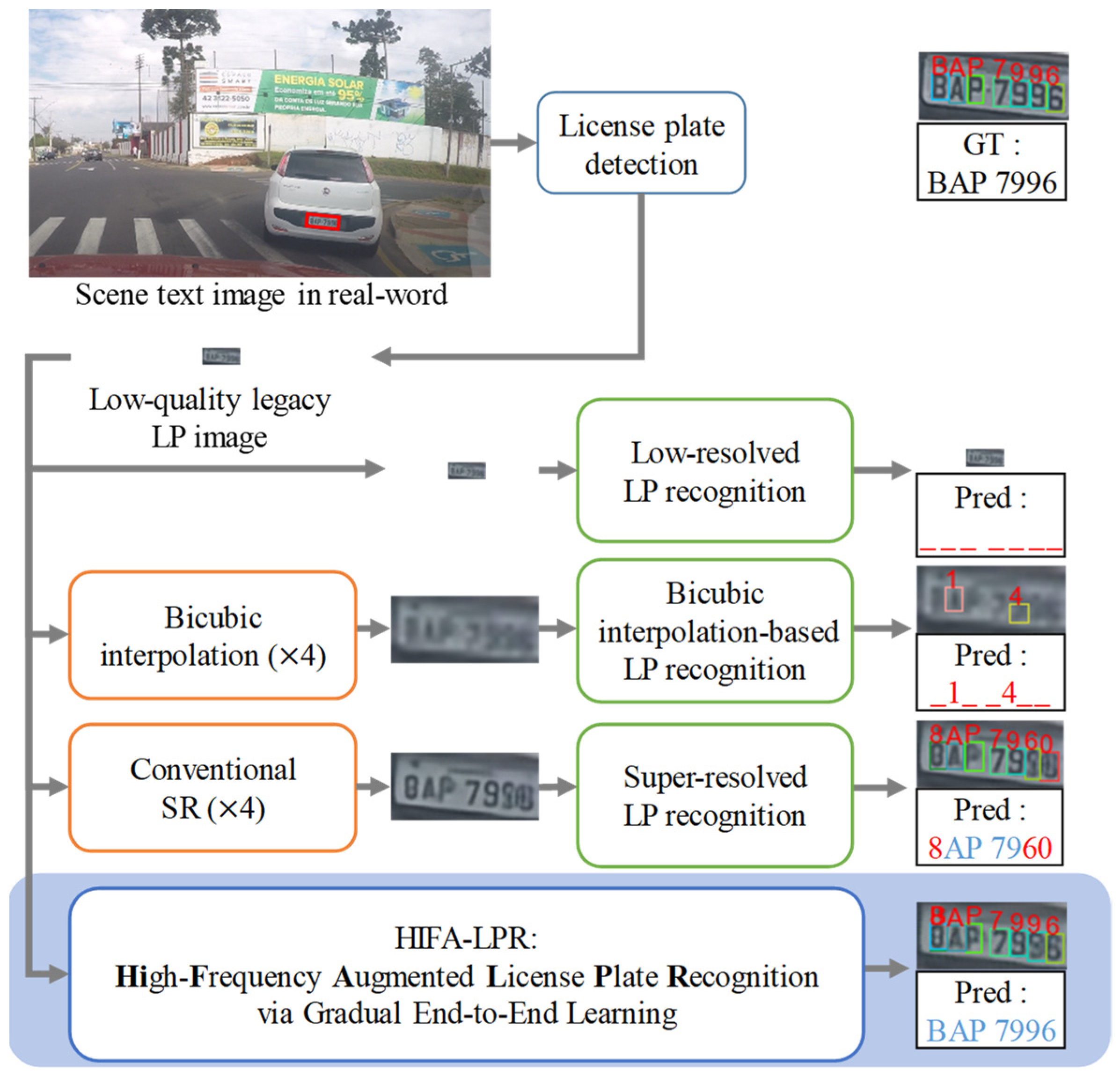
Figure 1.
Examples of LP recognition approaches in a real-world scenario. Our proposed HIFA-LPR model outperforms conventional approaches. “_” denotes a missing character recognition. Red character denotes incorrect prediction. Blue character denotes correct prediction. “GT” denotes ground truth. “Pred” denotes the prediction result.
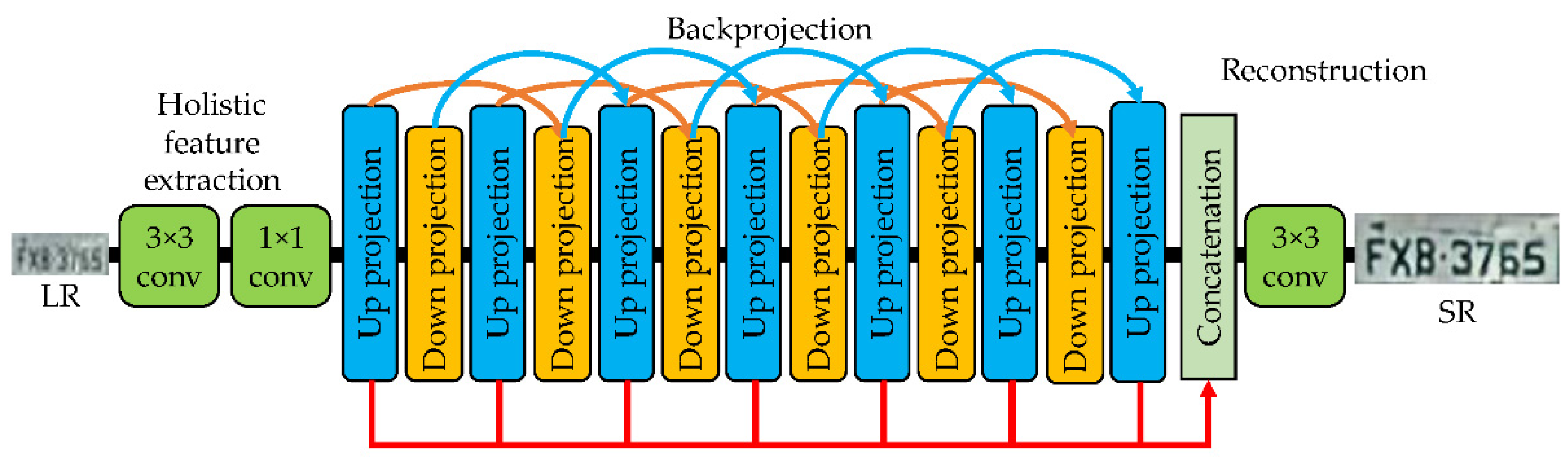
Figure 2.
Architecture of holistic-feature-extraction-based SR module.
Figure 2.
Architecture of holistic-feature-extraction-based SR module.
Figure 3.
(a) Diagram of the patch-based end-to-end training process. (b) Diagram of the holistic-feature-based end-to-end training process. In output images, red boxes denote the detected character region.
Figure 3.
(a) Diagram of the patch-based end-to-end training process. (b) Diagram of the holistic-feature-based end-to-end training process. In output images, red boxes denote the detected character region.
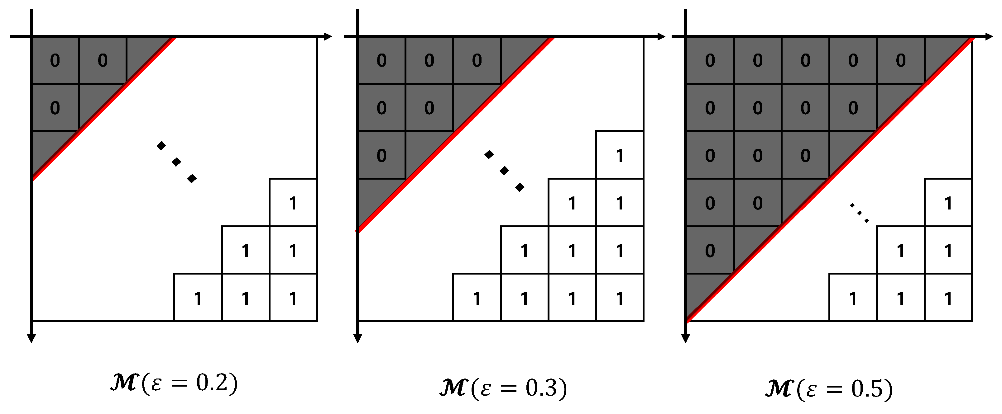
Figure 4.
Examples of according to . Because of the larger hyper-parameter , more low-frequency components are masked. We empirically set to 0.2.
Figure 4.
Examples of according to . Because of the larger hyper-parameter , more low-frequency components are masked. We empirically set to 0.2.
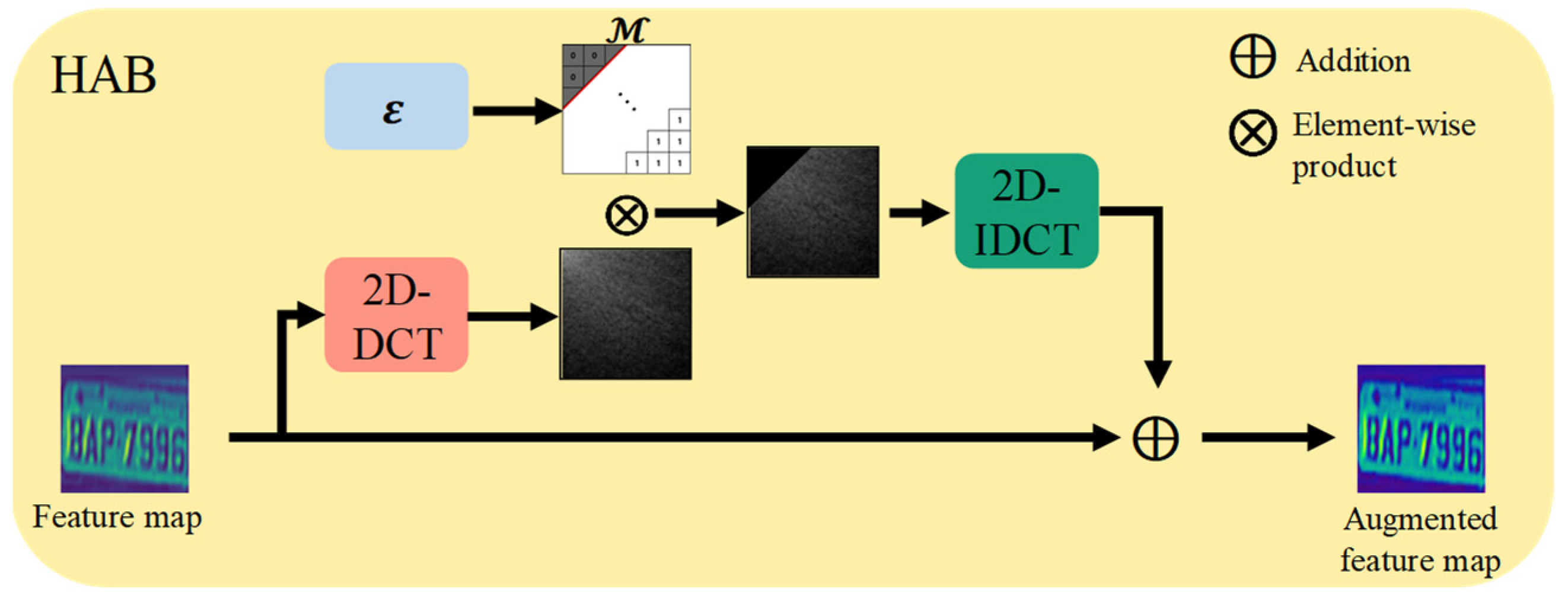
Figure 5.
Architecture of HAB.
Figure 5.
Architecture of HAB.
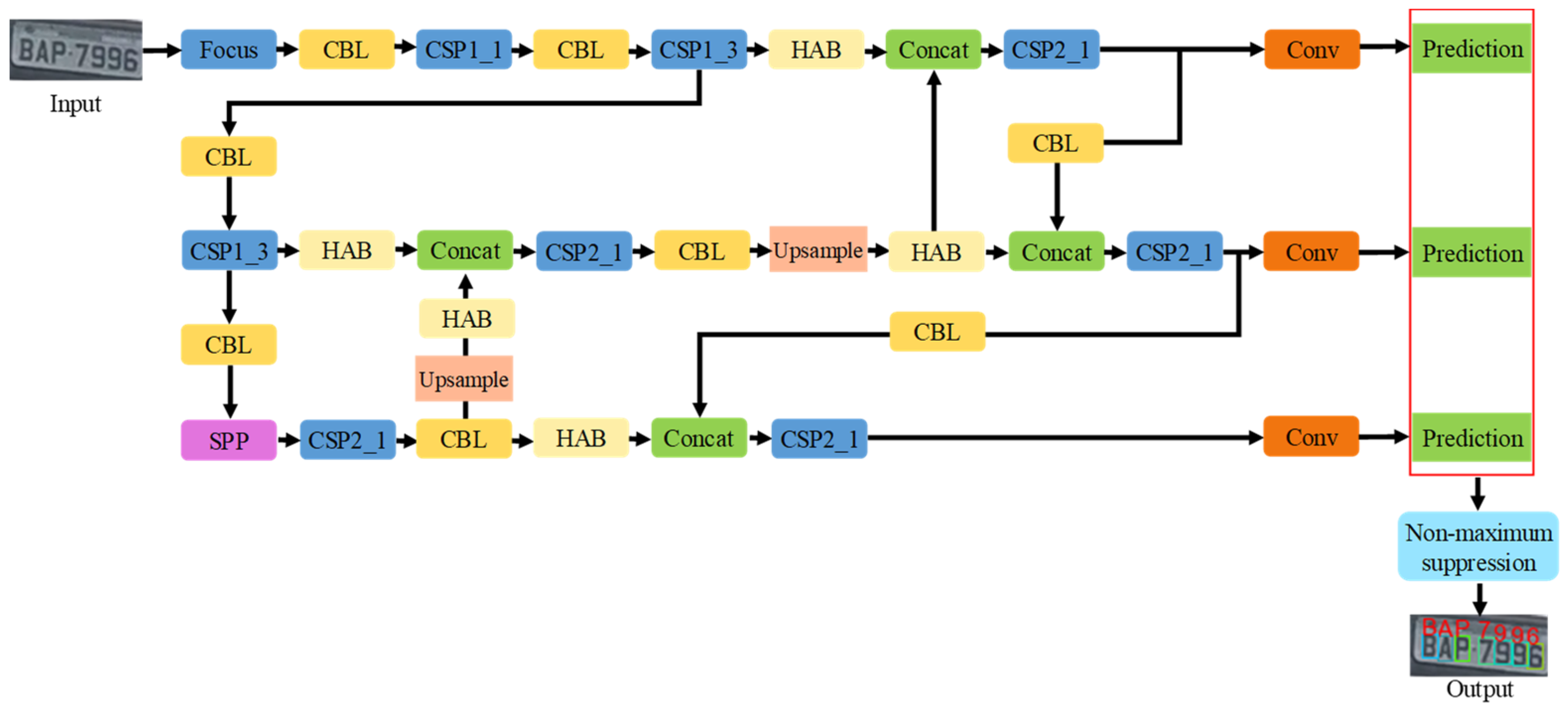
Figure 6.
Flowchart of LP recognition module based on high-frequency augmentation.
Figure 6.
Flowchart of LP recognition module based on high-frequency augmentation.
Figure 7.
Flowchart of gradual end-to-end learning method. (a) Step 1: Independent training of the SR module and LP recognition module. (b) Step 2: SR module training while freezing LP recognition module. (c) Step 3: LP recognition module training while freezing SR module. “GT” denotes ground truth. “Pred” denotes the prediction result.
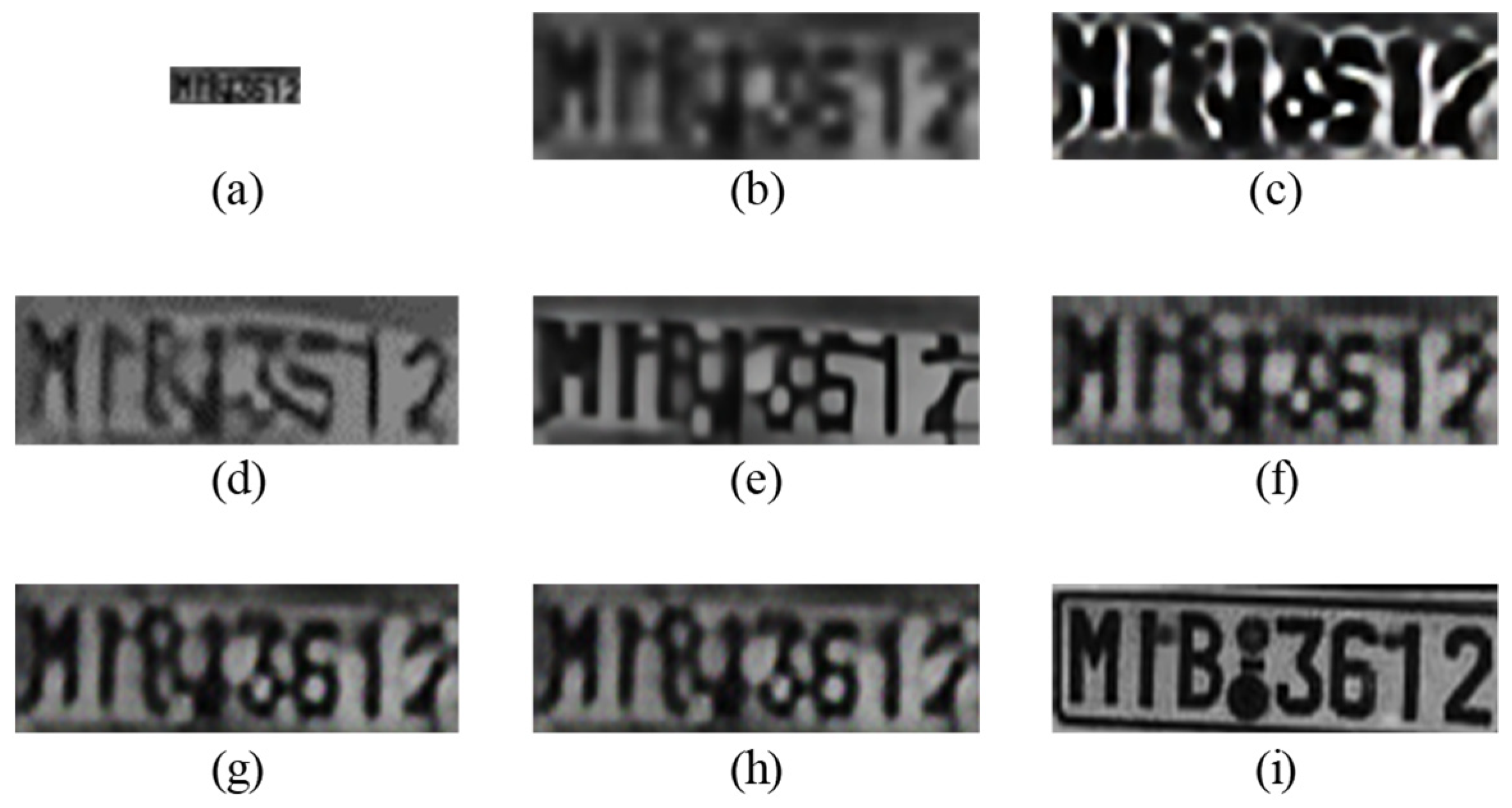
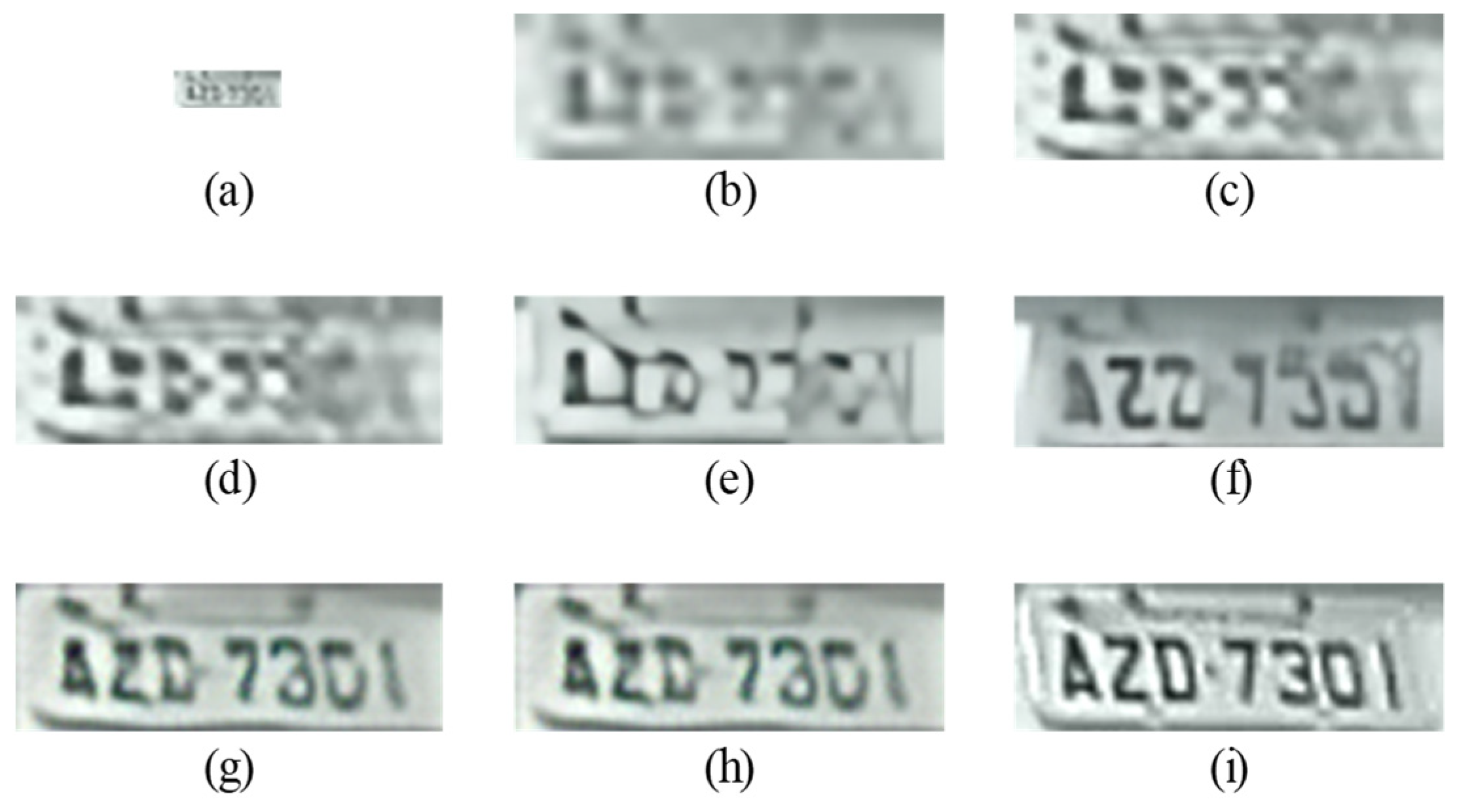
Figure 8.
SR results on the LP image of the UFPR dataset for scale factor (×3): (a) input low-quality legacy image (24 × 8), (b) bicubic (96 × 32), (c) MZSR, (d) DRN, (e) SwinIR, (f) HIFA-LPR (Step 1), (g) HIFA-LPR (Step 2), (h) HIFA-LPR (Step 3), (i) HR image.
Figure 8.
SR results on the LP image of the UFPR dataset for scale factor (×3): (a) input low-quality legacy image (24 × 8), (b) bicubic (96 × 32), (c) MZSR, (d) DRN, (e) SwinIR, (f) HIFA-LPR (Step 1), (g) HIFA-LPR (Step 2), (h) HIFA-LPR (Step 3), (i) HR image.
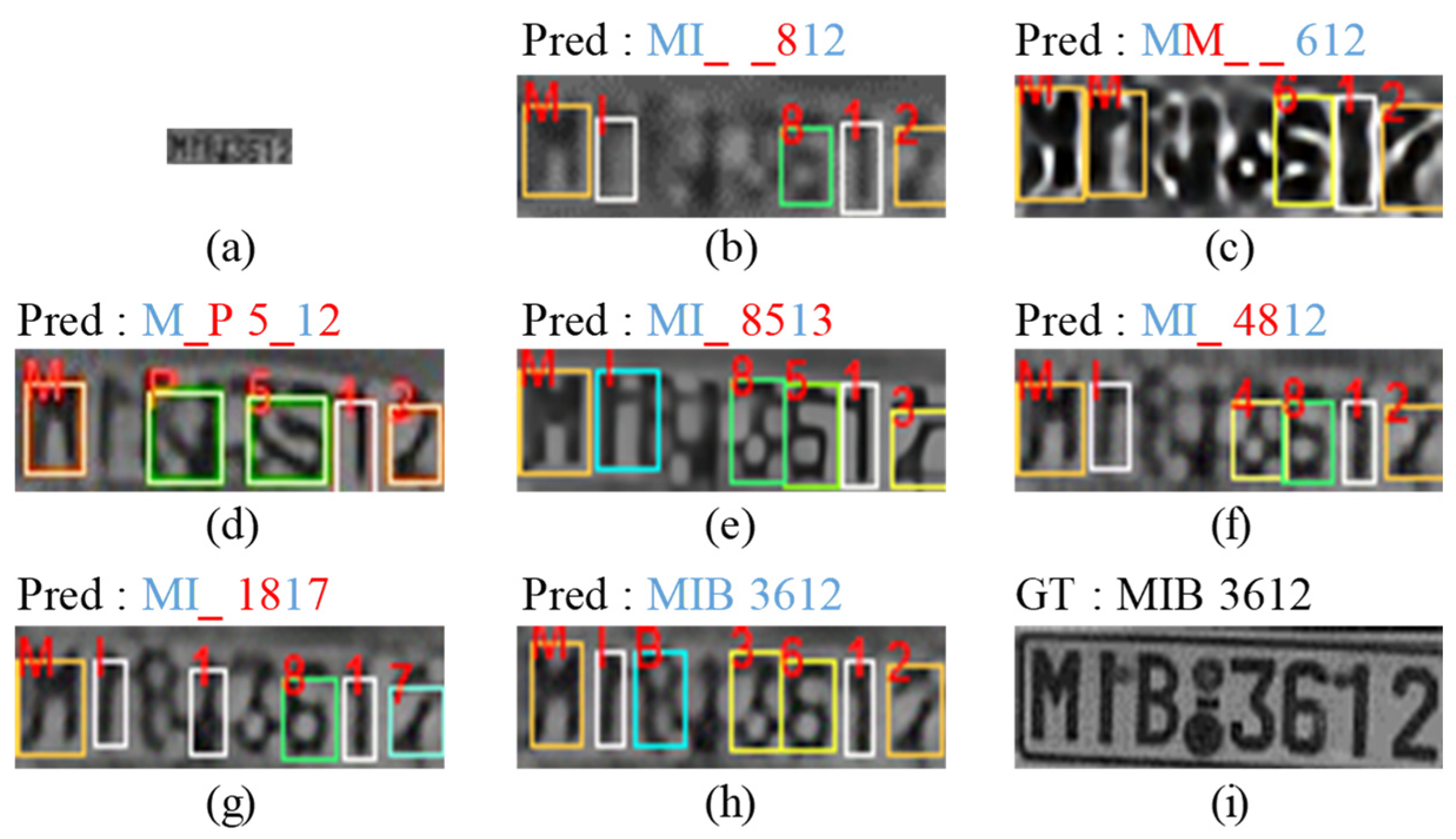
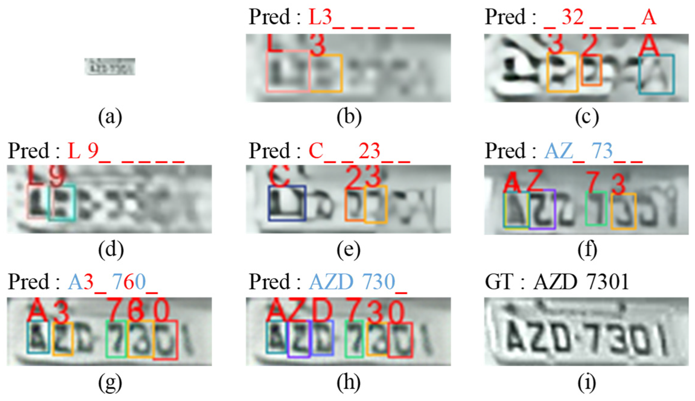
Figure 9.
LP recognition results on (a) input low-quality legacy image (24 × 8), (b) bicubic image (96 × 32), (c) MZSR result, (d) DRN result, (e) SwinIR result, (f) HIFA-LPR (Step 1) result, (g) HIFA-LPR (Step 2) result, (h) HIFA-LPR (Step 3) result, (i) HR image. “_” denotes a missing character. Red character denotes an incorrect prediction. Blue character denotes a correct prediction. “GT” denotes ground truth. “Pred” denotes the prediction result.
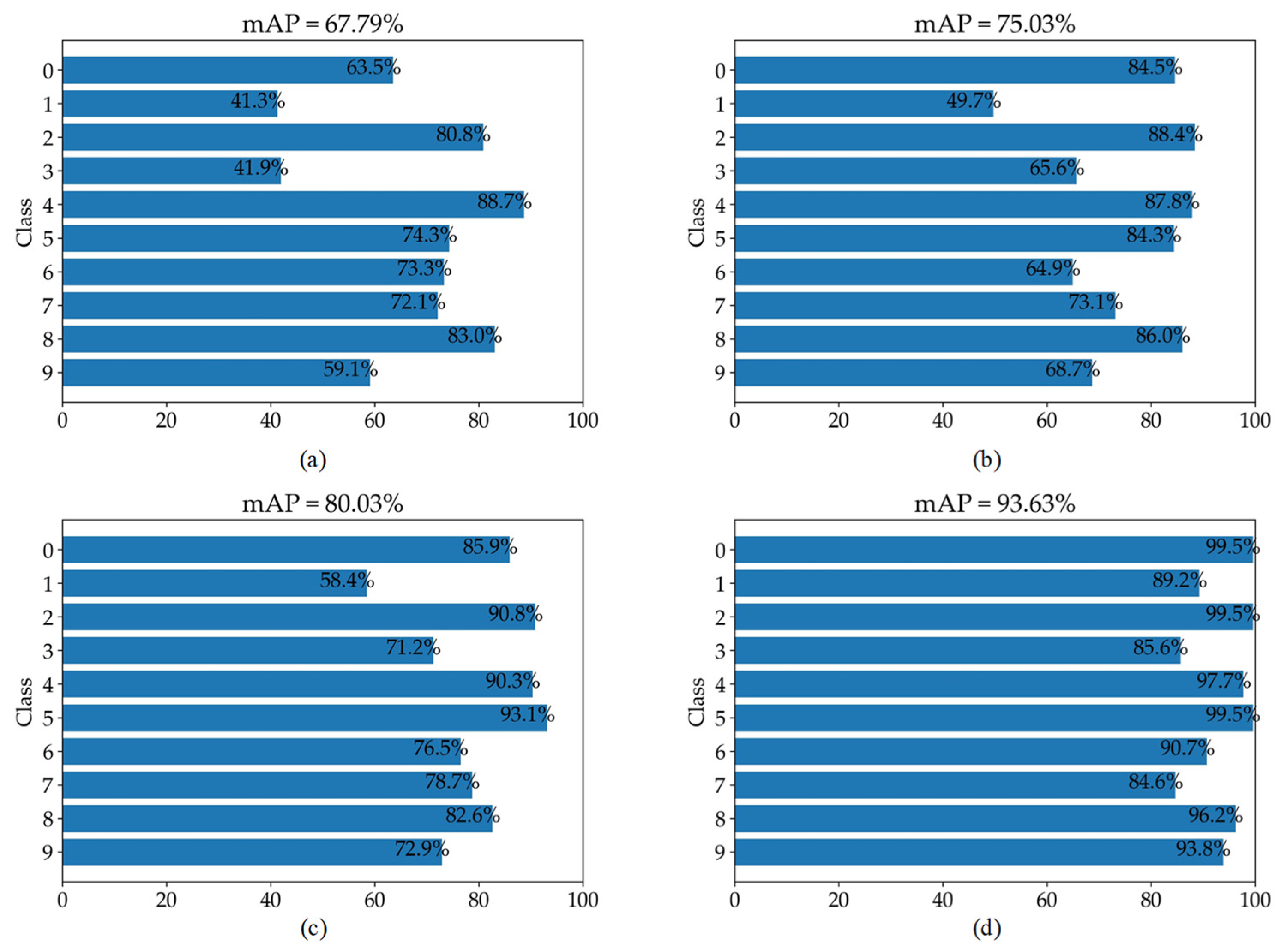
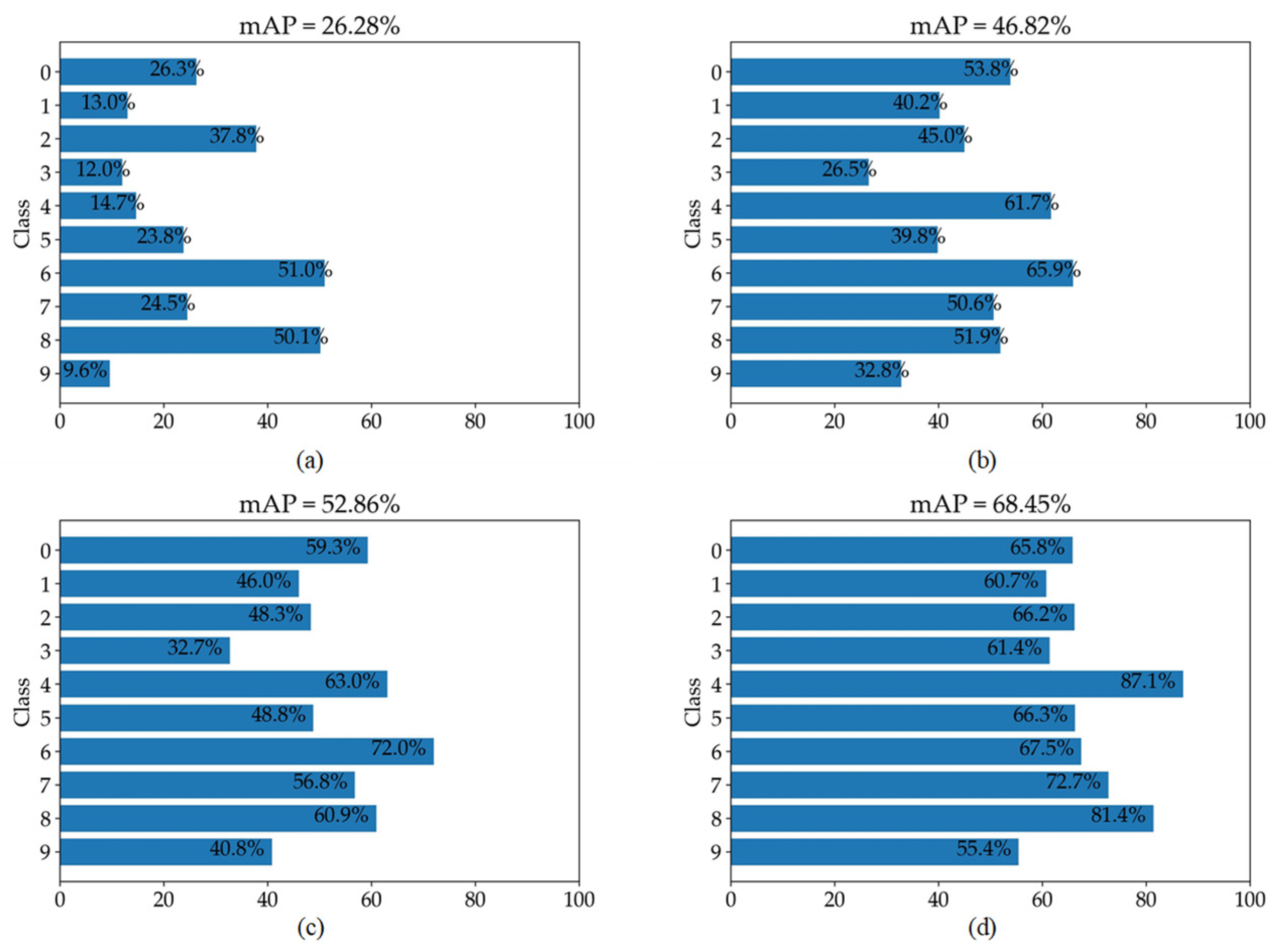
Figure 10.
mAP comparison results for only numbers (0–9) on the UFPR dataset for scale factor (×4). (a–d) represent the mAP results on bicubic results, HIFA-LPR (Step 1) results, HIFA-LPR (Step 2) results, and HIFA-LPR (Step 3) results, respectively.
Figure 10.
mAP comparison results for only numbers (0–9) on the UFPR dataset for scale factor (×4). (a–d) represent the mAP results on bicubic results, HIFA-LPR (Step 1) results, HIFA-LPR (Step 2) results, and HIFA-LPR (Step 3) results, respectively.
Figure 11.
SR results on the LP image of the Greek vehicle dataset for scale factor (×4): (a) input low-quality legacy image (24 × 8), (b) Bicubic (96 × 32), (c) MZSR, (d) DRN, (e) SwinIR, (f) HIFA-LPR (Step 1), (g) HIFA-LPR (Step 2), (h) HIFA-LPR (Step 3), (i) HR image.
Figure 11.
SR results on the LP image of the Greek vehicle dataset for scale factor (×4): (a) input low-quality legacy image (24 × 8), (b) Bicubic (96 × 32), (c) MZSR, (d) DRN, (e) SwinIR, (f) HIFA-LPR (Step 1), (g) HIFA-LPR (Step 2), (h) HIFA-LPR (Step 3), (i) HR image.
Figure 12.
LP recognition results on the Greek vehicle dataset with (a) input low-quality legacy image (28 × 8), (b) bicubic result (112 × 32), (c) MZSR result, (d) DRN result, (e) SwinIR result, (f) HIFA-LPR (Step 1) result, (g) HIFA-LPR (Step 2) result, (h) HIFA-LPR (Step 3) result. (i) HR image. “_” denotes a missing character. Red character denotes an incorrect prediction. Blue character denotes a correct prediction. “GT” denotes ground truth. “Pred” denotes the prediction result.
Figure 13.
mAP comparison results for only numbers (0–9) on the Greek vehicle dataset for scale factor (×4). (a–d) represent the mAP results on bicubic results, HIFA-LPR (Step 1) results, HIFA-LPR (Step 2) results, and HIFA-LPR (Step 3), respectively.
Figure 13.
mAP comparison results for only numbers (0–9) on the Greek vehicle dataset for scale factor (×4). (a–d) represent the mAP results on bicubic results, HIFA-LPR (Step 1) results, HIFA-LPR (Step 2) results, and HIFA-LPR (Step 3), respectively.
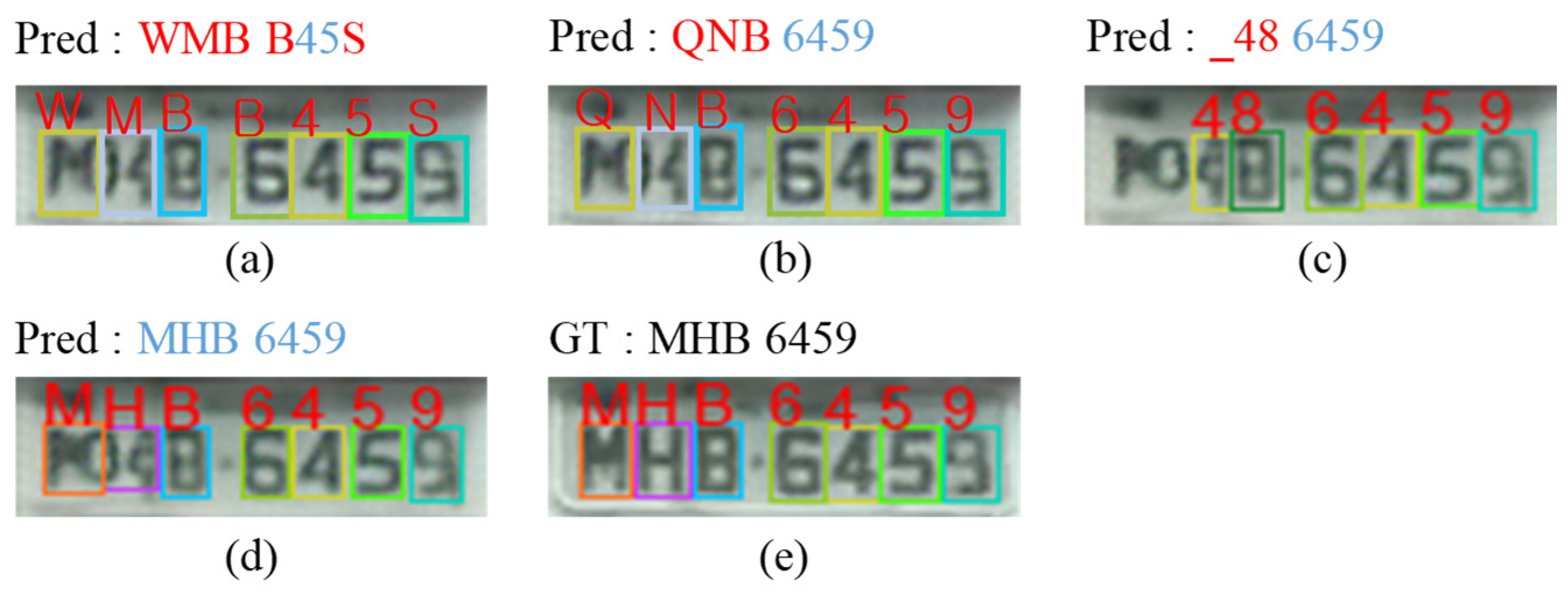
Figure 14.
LP recognition results on same SR result (80 × 60). (a) Tesseract-OCR result, (b) OpenALPR result (c) Yolov5 result, (d) HIFA-LPR result, (e) HR image. “_” denotes a missing character. Red character denotes an incorrect prediction. Blue character denotes a correct prediction. “GT” denotes ground truth. “Pred” denotes the prediction result.
Table 1.
Comparison between the HIFA-LPR model and other existing approaches for scale factor (×3) on the UFPR dataset.
Table 1.
Comparison between the HIFA-LPR model and other existing approaches for scale factor (×3) on the UFPR dataset.
| PSNR and mAP on UFPR Validation Dataset |
|---|
| Method | PSNR (dB) | mAP (%) |
|---|
| SR Module | Recognition Module |
|---|
| LR baseline | Tesseract-OCR [14] | - | 17.8 |
| Bicubic | 24.10 | 29.1 |
| MZSR [11] | 17.64 | 22.7 |
| DRN [8] | 25.11 | 33.3 |
| SwinIR [12] | 25.66 | 36.4 |
| LR baseline | Yolov5 [29] | - | 49.9 |
| Bicubic | 24.10 | 50.1 |
| MZSR [11] | 17.64 | 43.7 |
| DRN [8] | 25.11 | 58.5 |
| SwinIR [12] | 25.66 | 61.1 |
| HIFA-LPR (Step 1) | 26.40 | 62.7 |
| HIFA-LPR (Step 2) | 27.20 | 67.7 |
| HIFA-LPR (Step 3) | 27.20 | 82.4 |
Table 2.
Comparison between the HIFA-LPR model and other existing approaches for scale factor (×4) on the UFPR dataset.
Table 2.
Comparison between the HIFA-LPR model and other existing approaches for scale factor (×4) on the UFPR dataset.
| PSNR and mAP on UFPR Validation Dataset |
|---|
| Method | PSNR (dB) | mAP (%) |
|---|
| SR Module | Recognition Module |
|---|
| LR baseline | Tesseract-OCR [14] | - | 12.7 |
| Bicubic | 22.18 | 18.8 |
| MZSR [11] | 17.99 | 11.2 |
| DRN [8] | 22.74 | 19.7 |
| SwinIR [12] | 23.33 | 21.8 |
| LR baseline | Yolov5 [29] | - | 32.4 |
| Bicubic | 22.18 | 35.8 |
| MZSR [11] | 17.99 | 27.3 |
| DRN [8] | 22.74 | 36.7 |
| SwinIR [12] | 23.33 | 38.1 |
| HIFA-LPR (Step 1) | 23.77 | 34.4 |
| HIFA-LPR (Step 2) | 23.91 | 42.2 |
| HIFA-LPR (Step 3) | 23.91 | 60.9 |
Table 3.
Comparison between the HIFA-LPR model and other existing approaches for scale factor (×3) on the Greek vehicle dataset.
Table 3.
Comparison between the HIFA-LPR model and other existing approaches for scale factor (×3) on the Greek vehicle dataset.
| PSNR and mAP on Greek Vehicle Validation Dataset |
|---|
| Method | PSNR (dB) | mAP (%) |
|---|
| SR Module | Recognition Module |
|---|
| LR baseline | Tesseract-OCR [14] | - | 48.2 |
| Bicubic | 21.33 | 60.3 |
| MZSR [11] | 16.07 | 47.2 |
| DRN [8] | 25.08 | 70.4 |
| SwinIR [12] | 25.58 | 74.7 |
| LR baseline | Yolov5 [29] | - | 72.1 |
| Bicubic | 21.33 | 92.1 |
| MZSR [11] | 16.07 | 91.8 |
| DRN [8] | 25.08 | 95.9 |
| SwinIR [12] | 25.58 | 96.8 |
| HIFA-LPR (Step 1) | 21.43 | 91.9 |
| HIFA-LPR (Step 2) | 22.65 | 94.4 |
| HIFA-LPR (Step 3) | 22.65 | 98.3 |
Table 4.
Comparison between the HIFA-LPR model and other existing approaches for scale factor (×4) on the Greek vehicle dataset.
Table 4.
Comparison between the HIFA-LPR model and other existing approaches for scale factor (×4) on the Greek vehicle dataset.
| PSNR and mAP on Greek Vehicle Validation Dataset |
|---|
| Method | PSNR (dB) | mAP (%) |
|---|
| SR Module | Recognition Module |
|---|
| LR baseline | Tesseract-OCR [14] | - | 27.4 |
| Bicubic | 21.33 | 31.1 |
| MZSR [11] | 16.07 | 22.3 |
| DRN [8] | 25.08 | 52.1 |
| SwinIR [12] | 25.58 | 55.1 |
| LR baseline | Yolov5 [29] | - | 57.1 |
| Bicubic | 19.63 | 77.3 |
| MZSR [11] | 15.96 | 74.1 |
| DRN [8] | 23.83 | 87.5 |
| SwinIR [12] | 23.61 | 89.1 |
| HIFA-LPR (Step 1) | 20.01 | 75.2 |
| HIFA-LPR (Step 2) | 20.60 | 80.6 |
| HIFA-LPR (Step 3) | 20.60 | 90.5 |
Table 5.
Comparison between the patch extraction-based SR and the holistic extraction-based SR for scale factor (×4) on the UFPR dataset.
Table 5.
Comparison between the patch extraction-based SR and the holistic extraction-based SR for scale factor (×4) on the UFPR dataset.
| PSNR and mAP on UFPR Validation Dataset |
|---|
| Method | PSNR (dB) | mAP (%) |
|---|
| SR Module | Recognition Module |
|---|
| Patch-extraction-based SR | Yolov5 [29] | 23.77 | 34.4 |
| Holistic-extraction-based SR | 24.65 | 44.7 |
Table 6.
Comparison between the LP recognition module based on high-frequency augmentation and other modules for scale factor (×4) on the UFPR dataset.
Table 6.
Comparison between the LP recognition module based on high-frequency augmentation and other modules for scale factor (×4) on the UFPR dataset.
| PSNR and mAP on UFPR Validation Dataset |
|---|
| Method | mAP (%) |
|---|
| Tesseract-OCR [14] | 19.1 |
| Yolov5 [29] | 34.4 |
LP recognition module without
high-frequency augmentation | 57.2 |
LP recognition module with
high-frequency augmentation | 60.9 |


