This section will study the set of periods of 3-IETs for two different permutations with one flip, namely and . Our study shows that one must use different techniques to compute the periods of T. Of course, this fact is an additional problem for the characterization of periods of general IETs.
5.1. The Permutation
Note that this map is defined as
First, we prove the following result.
Lemma 4. The 3-IET T with permutation has a fixed point if and only if .
Proof. T has a fixed point is
. The fixed point is
but note that it has to be greater than
. This condition reads as
which implies easily
Since the proof works in both directions, it concludes. □
Assume that
so that
T has a fixed point. Then, the interval
and contains the fixed point of
T. In addition,
and so, the length of
. Let
. Normalizing
,
and
, we define
to have permutation
and length vector
. Then, we have the following result.
Theorem 13. Under the above notation, assume that . Then
If for some , then .
If , then .
Proof. Note that all the points of
J are periodic with period one or two. Since
J is invariant by
T so are the subintervals of
. Then, the map
is well defined and we have that
. In addition,
is given by the expression
By Theorem 8, we check that the periods of are either when for some or when . Then, the proof concludes. □
Theorem 13 characterizes the set of periods of T when even when the components , and are not rationally dependent. Now, we assume that , and , for some . If , then we can find such that write , and .
Since Theorem 13 characterizes the periods of
T such that
, we focuss our attention to the case
. It is easy to realize that
T is a variation of the rotation of the circle
. Only the interval
is modified to reverse the orientation. We consider the map
T defined on
as follows
Note that this can be done by the conjugacy that carries
into
in a linear way. We label the subinterval
by
j,
. It is immediate to see that if
, then
On the other hand, for
we check that the iteration of the interval labeled with
is given by
Recall that
and note that
for
, whew
R is the rotation
.
Now, fixed
i, for any
we consider the equation
which tells us the time
X needed for the rotation
R to go from interval
to
, which reads as
In the following, we will use a series of fundamental results on congruences. First, the reader is referred to ([
25], Chapter 5) for an account of the topic and the resolution of linear congruences. The Equation (
9) has solution
if and only if
divides
. Clearly,
when
. We construct the matrix
, where
is either the solution of the equation or the symbol *, here used to state that there is not solution and therefore the intervals
and
are not map one into the other by the rotation
R.
Now, we distinguish two cases. If
, then the Equation (
9) always have a unique solution given by
where
is the Euler function given by
If
, then the Equation (
9) has a solution if and only if
d divides
. It has
d different solutions, the smaller one can be computed by solving the equation
that is, the solution will be
Hence, we can compute the set of periods of T in some particular cases as follows.
Theorem 14. Let . Then:
- (a)
If , then
- (b)
If ,
Proof. With the notation above,
and therefore,
T moves the intervals
,
like the rotation
given by
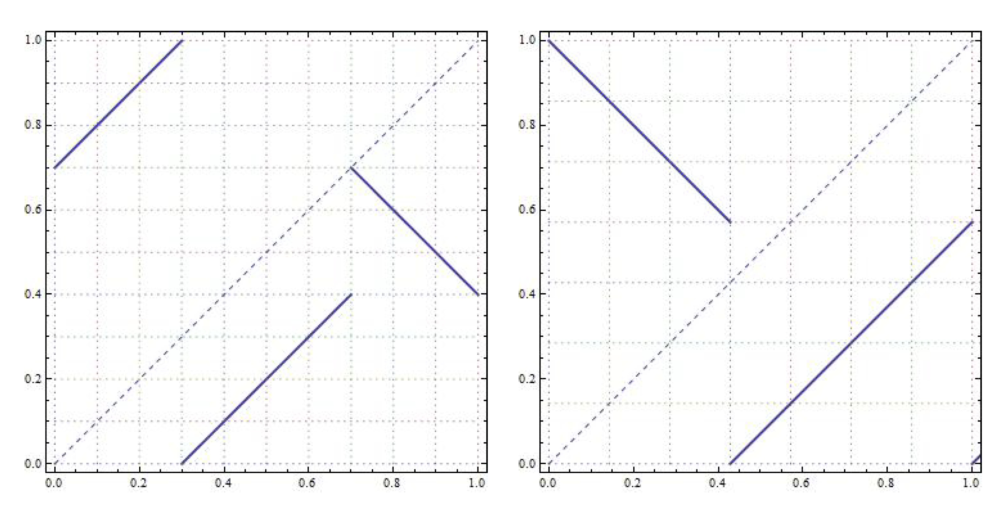
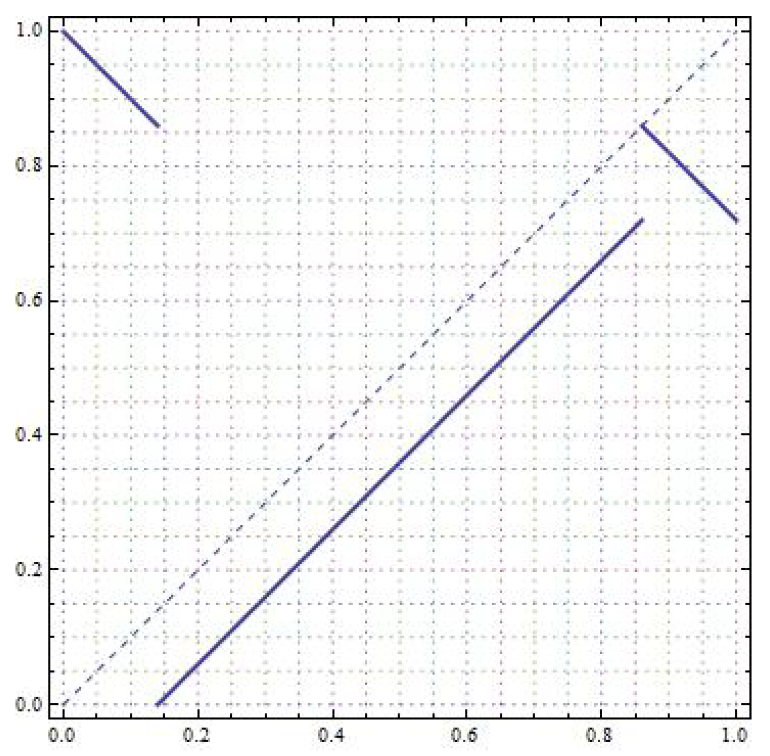
. Note that
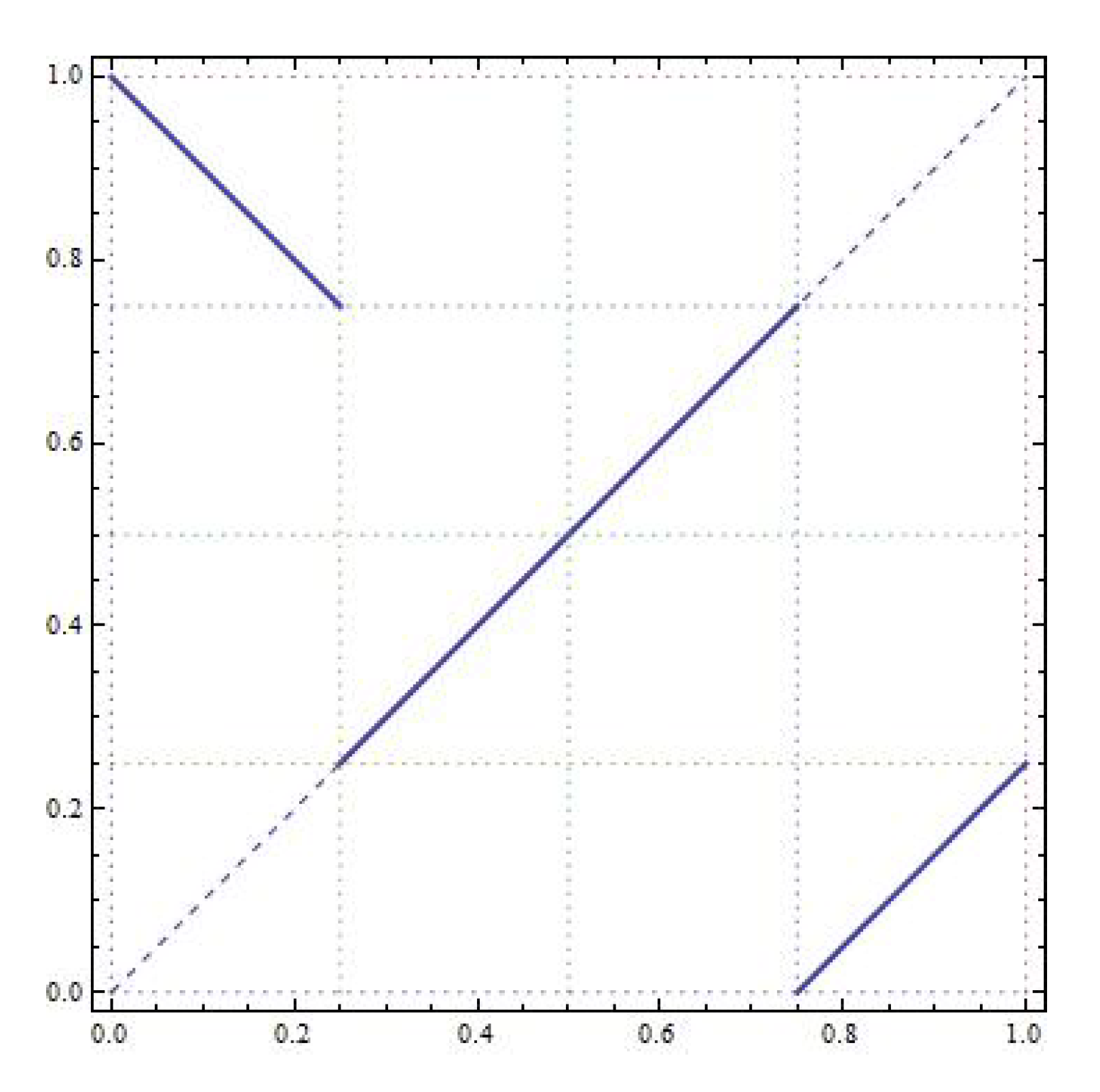
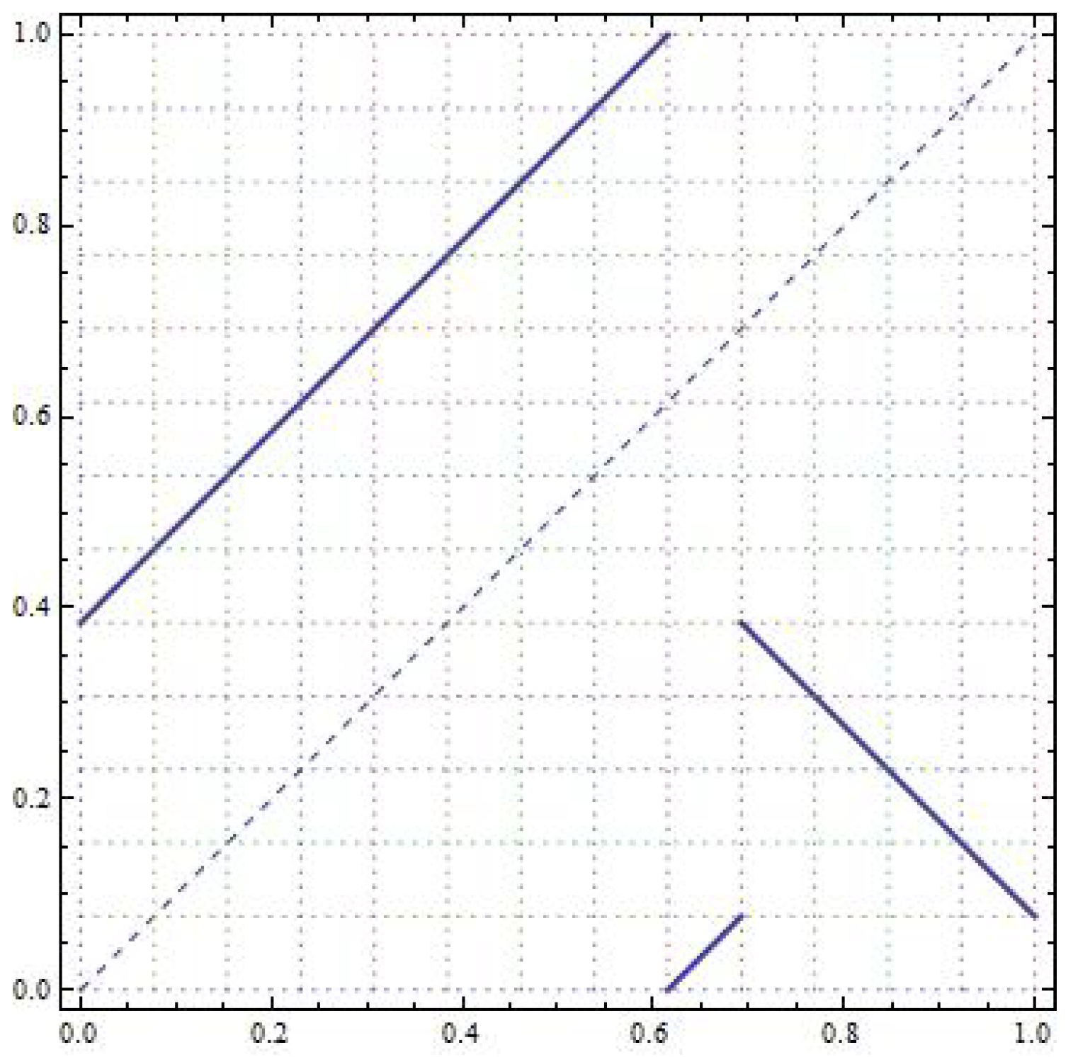
. See
Figure 11 to see the differences between the map
T and the rotation
R.
Note that
and thus Equation (
9) reads as
which obviously has always solution. If
, then the solution is unique and equal to
because
Then
, and since the image of interval
has negative slope, we have that
. This finishes the proof of (a). To prove (b), we take the equation
Reasoning as above, we find that . Finally, for the rest of intervals j in not included in the orbit of note that T acts as the rotation R and therefore the period associated to the interval j is . Then, and the proof concludes. □
Theorem 15. Let . Then:
- (a)
If , then , whereand In addition, , with .
- (b)
If ,
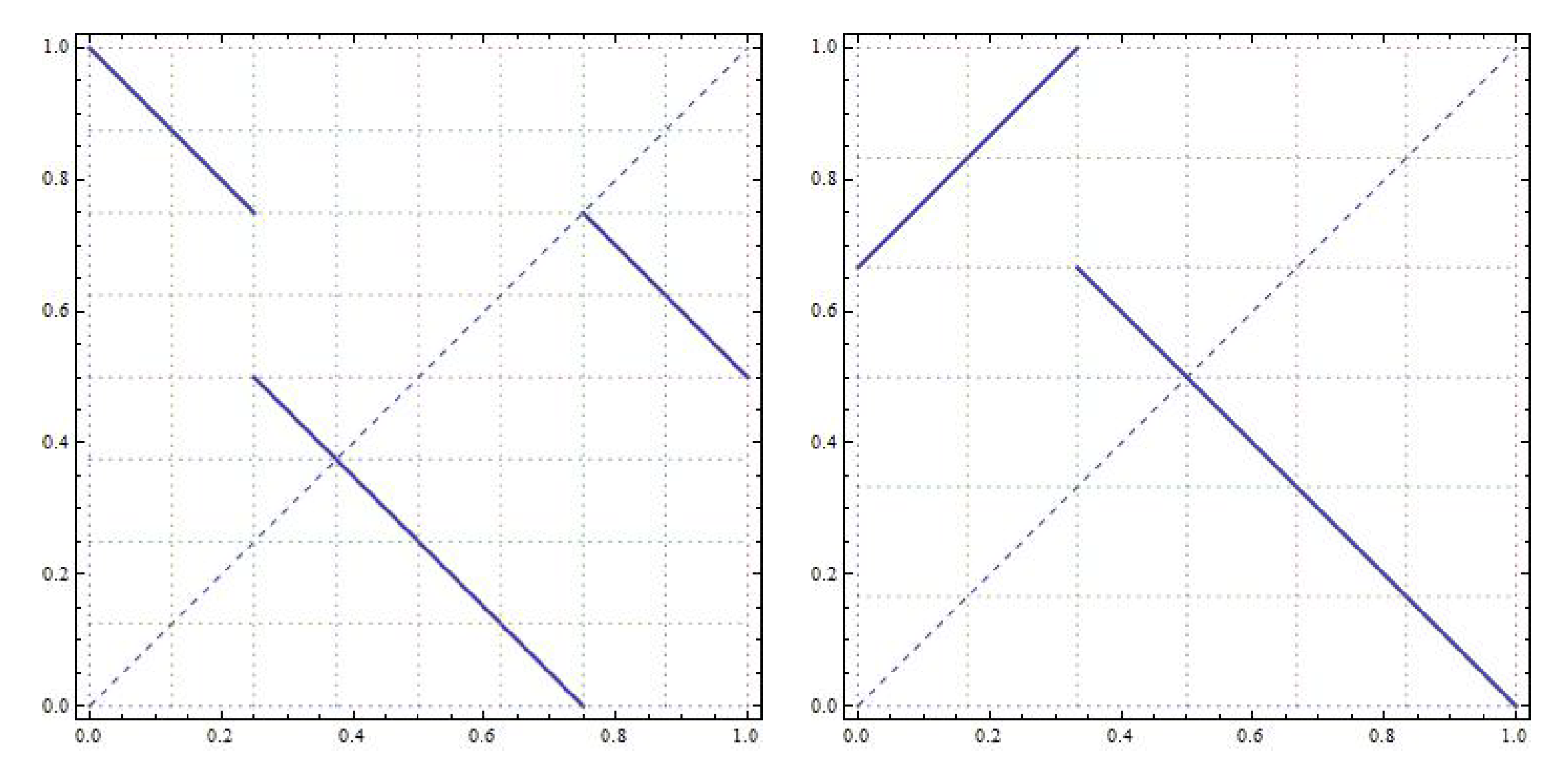
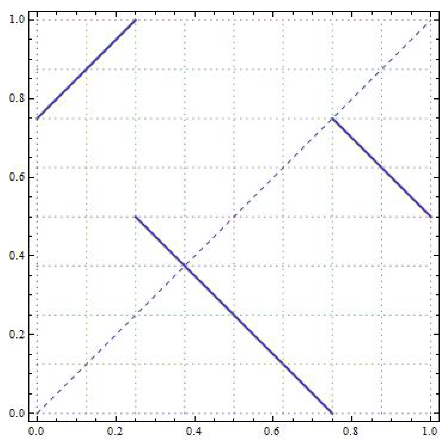
Proof. We can see
T on
as the rotation
.
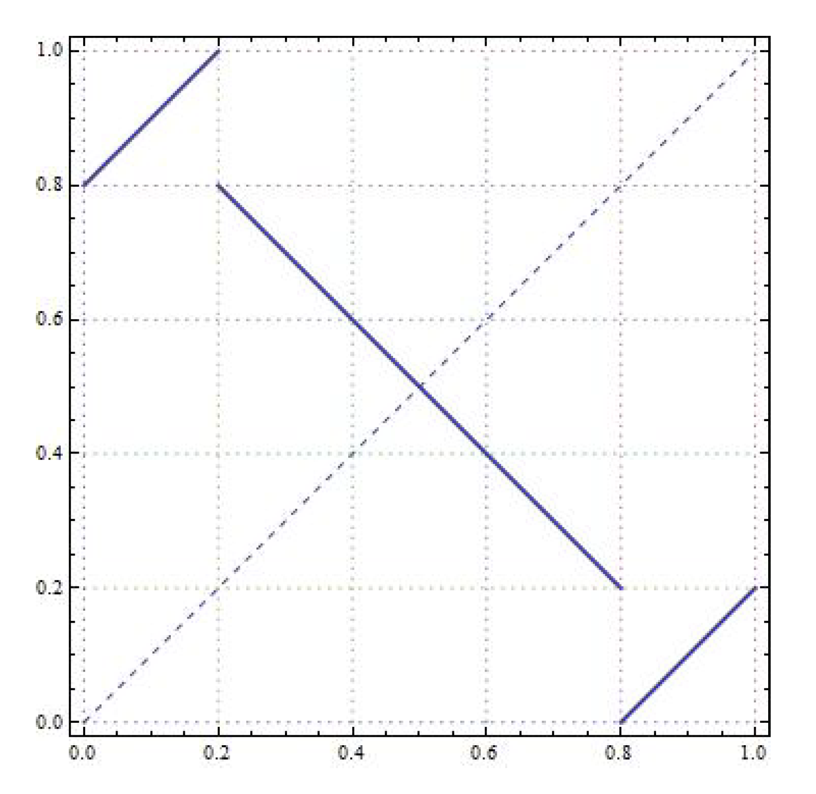
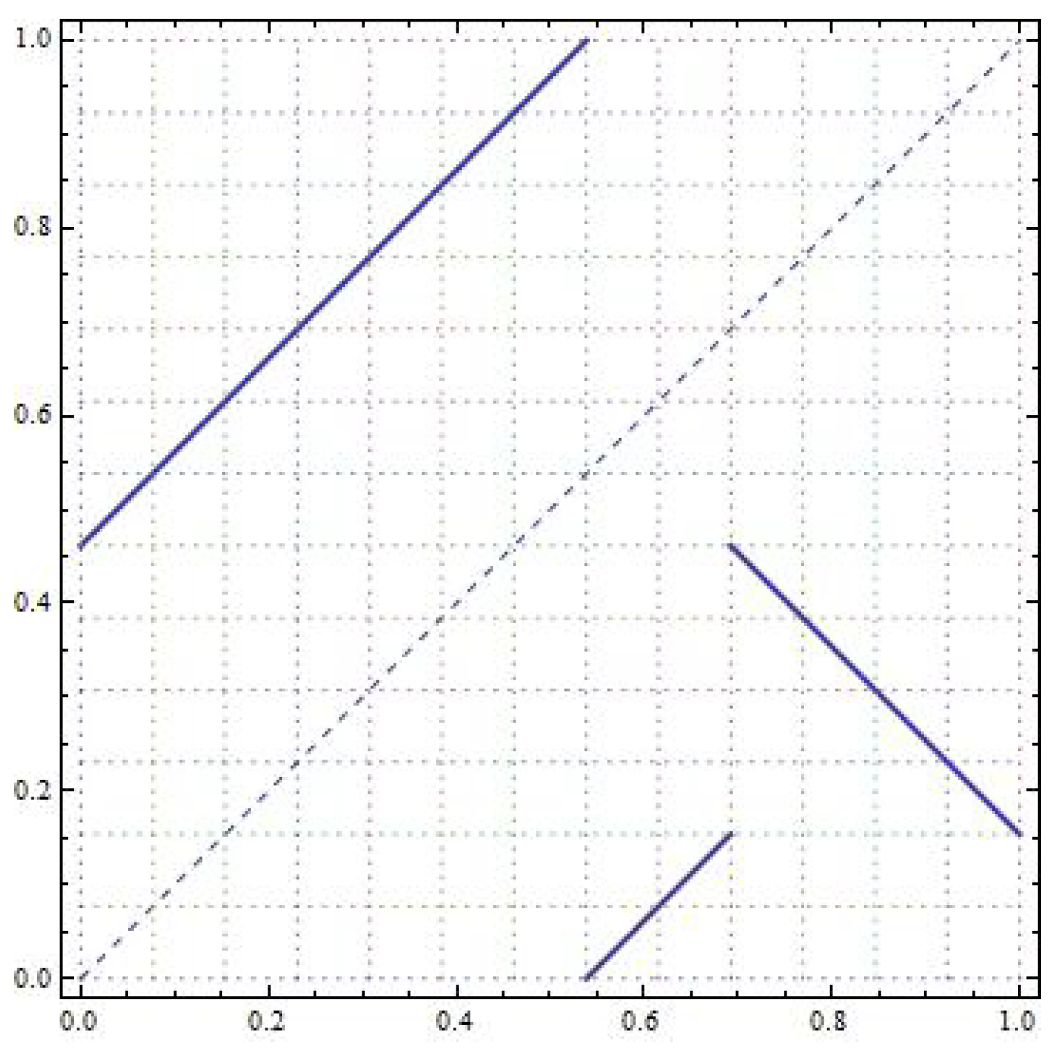
Figure 12 shows the differences between the maps
T and
R.
Note that
and thus Equation (
9) gives us three equations, namely
and
Now, we prove (a). Reasoning as in Theorem 14, we know that Equation (
11) has solution
. Thus, since the numbers
are generated in function of the dynamics of rotation
, which moves the indices forming a periodic orbit of period
m, necessarily the solutions
and
are smaller than
. Then,
and
have to be in
. As the slope of
T on the subintervals
and
is negative, then
. Note also that
(if
was equal to
, then
would be equal to
and the two linear congruences (10) and (11) would be satisfied. Then, subtracting these equations we would obtain
, which is impossible because
). To check that
, note that
where we have used the development of Newton’s binomial, and the facts that
is even for all
and
. Similarly
Now, we prove (b). Equation (
11) has solution because
d divides
. However,
d does not divide
and
and thus Equations (
10) and (
12) do not have any solution. Then the matrix
Then, the subinterval formed with subintervals and is periodic of period and with negative slope, which implies that . For the rest of intervals outside of , since no other periods are possible for the rotation , we conclude the proof. □
Theorem 16. Let . Then:
- (a)
If , then , where eitherandorand In addition, either or
- (b)
If , then:
- (b1)
If , then .
- (b2)
If , then whereand
Proof. Note that
and thus Equation (
9) gives us three equations, namely
Now, we prove (a). We know that Equation (
15) has the unique solution
. Then the matrix
has the form
Since the rotation R moves the intervals j in a periodic manner, with period m, we deduce that . Since and R is m-periodic, the orbit of the subinterval under T must be combined with either or . Thus, either or (note that since and , otherwise it would imply that subintervals and would be periodic without any combination with subinterval , and this is not possible). If , then the subintervals and form a periodic subinterval with period and negative slope, which implies that . Then, the subinterval is periodic with period and so . Similarly, we reasoning with the case to conclude that . Note that it is not possible to have periodic intervals outside because they would have to have period m. Then, either (if ) or (if ). The values of and are obtained as in the proof of Theorem 15, and the proof of (a) concludes.
Now, we prove (b). If
, then, solving the linear congruences we obtain the matrix
Note that Equations (
13) and (
17) have solution if and only if
. This is the case (b2), in which
, where
and
On the other hand,
and thus
.
In the case (b1),
, the matrix is
and thus
, and the proof concludes. □
The case
presents a variation. By Theorem 2, we can have at most three sets of the form
, for some positive integer
m, belonging to the set of periods of
T. However, now we have four subintervals with a negative slope, and we must figure out how they join. The procedure is as before. Here, we can see
T on
as the rotation
. However, now, in the interval
, we have four subintervals with a negative slope, so that we write the matrix
Assume first that . The smallest entries of the matrix will provide the periods of T. Below, we show several examples.
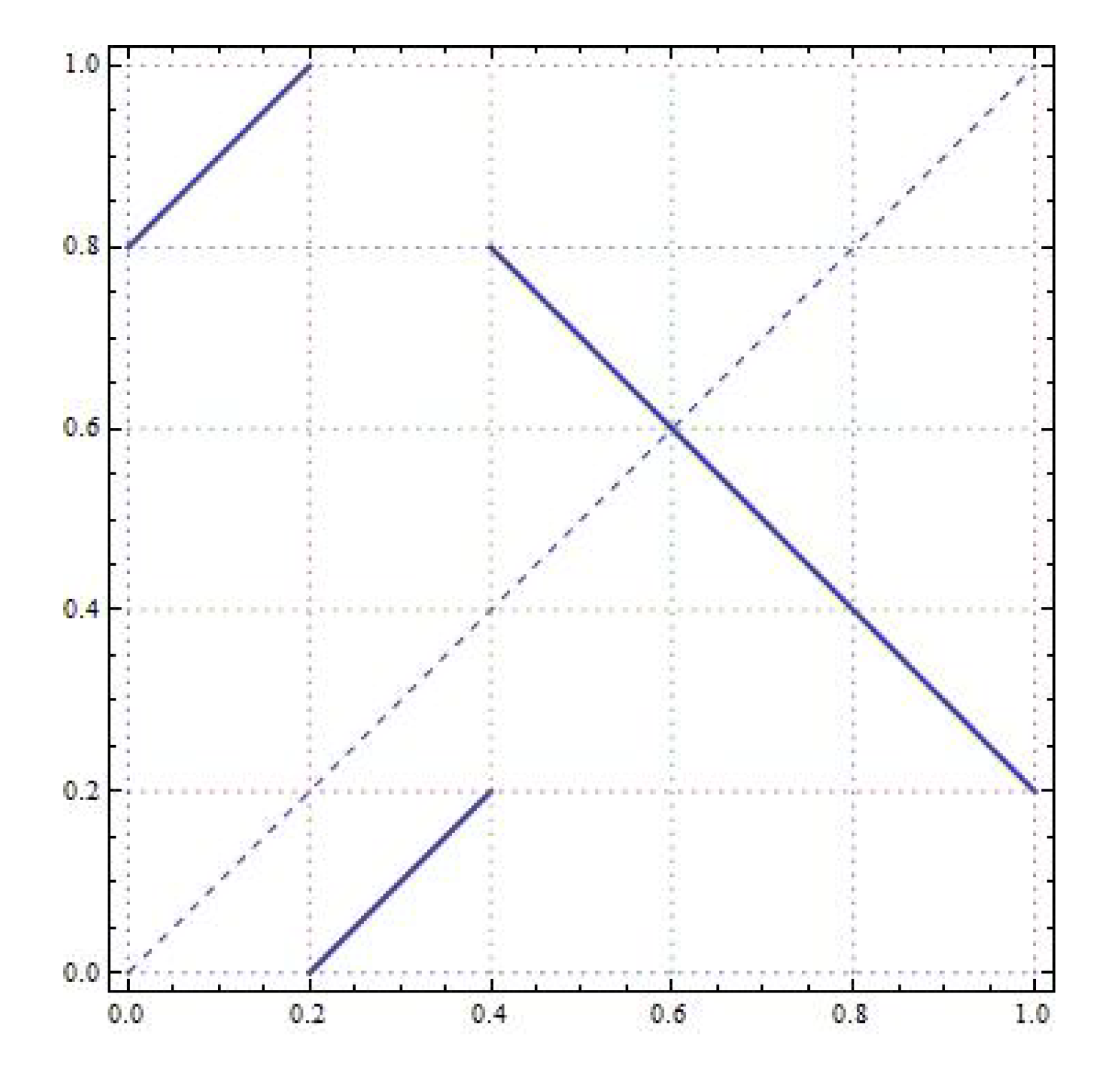
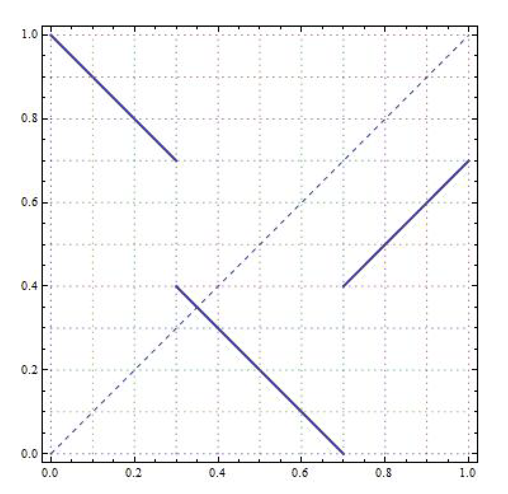
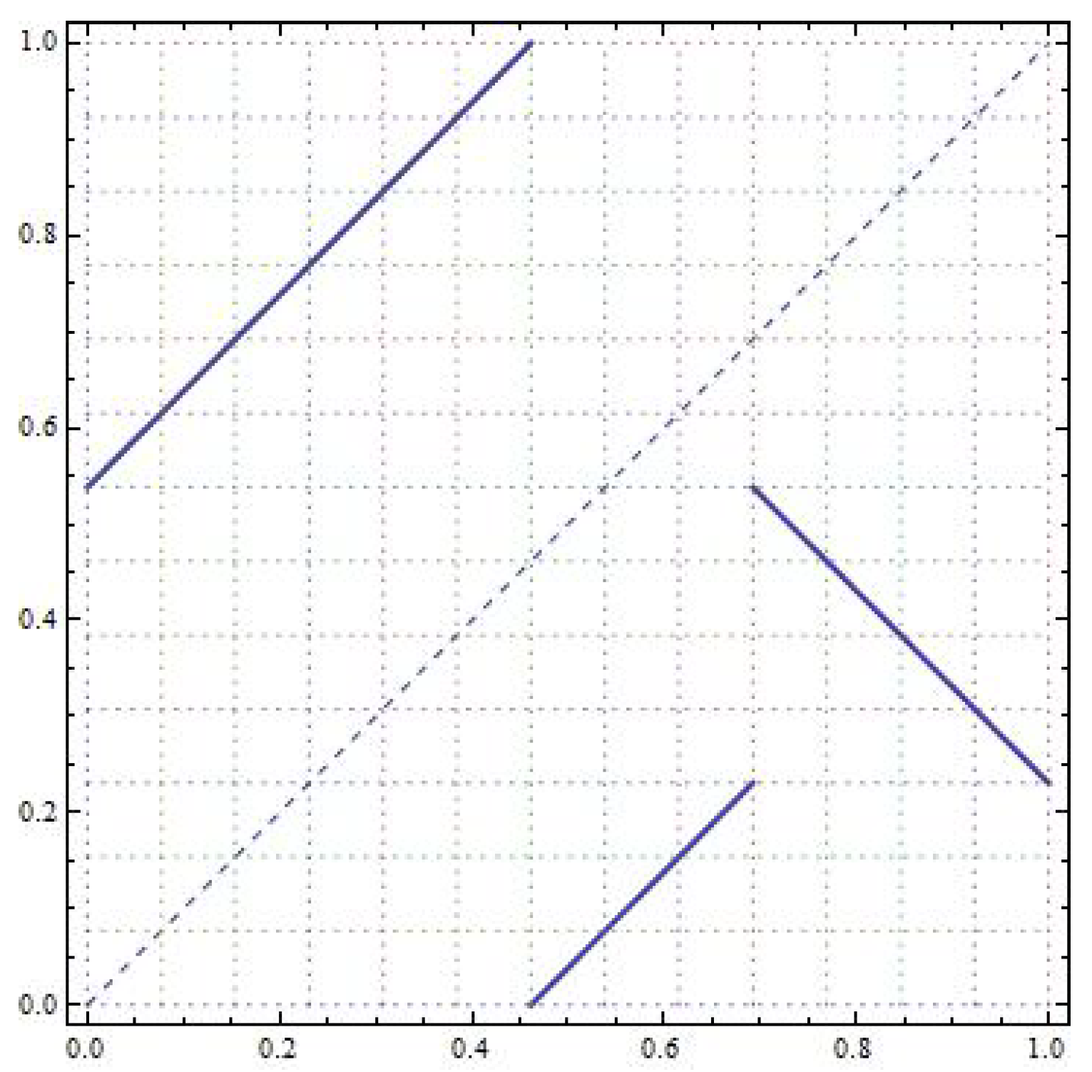
Example 2. Let and the length vector . Figure 13 shows the graph of T in which one can check the loops that give rise to the set of periods. We write the matrix The element gives us a loop of length 2 with a negative slope, so . The elements gives us a loop of length 6 with a positive slope, so the period 6. However, note that subintervals 11 and 12 are contiguous. Both forms a loop of of length 3 and negative slope, and so the set of periods . Finally, the element forms a loop of length 5 and negative slope, and so the set of periods . Thus .
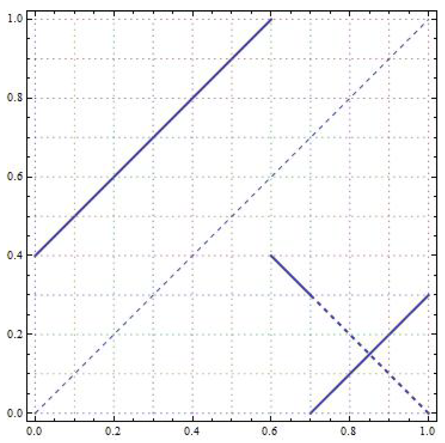
Example 3. Let and the length vector . Figure 14 shows the graph of T in which one can check the loops that give rise to the set of periods. We write the matrix The element gives us a loop of length 2 with a negative slope, so . The elements gives us a loop of length 4 with a positive slope, so the period 4. However, the subintervals 9, 10 and 11 are contiguous and hence, they form a loop of of length 2 and negative slope, and so . We use 6 subintervals to create this loop. The elements informs us of the existence of a loop of length 6 and positive slope, and so the period . However, we use six subintervals, and one would remain, which is impossible because it has to be periodic. The element gives again a loop of length six, which is not possible. Anyway, note that we cannot use these values because we already used the intervals 9, 10 and 11. So, the next element available is , which gives a loop of length 7 with a negative slope. Thus .
Example 4. Let and the length vector . Figure 15 shows the graph. We write the matrix The element gives us a loop of length 2 with a negative slope, so we obtain the periods . On the other hand, the elements gives us a loop of length 4 with a positive slope, so the period 4. However, note that subintervals 10, 11 and 12 are contiguous. Thus, they form a loop of of length 2 and negative slope, and so the set of periods . The next element available is , which gives a loop of length 7 with a negative slope. Thus .
In a similar way, we can check that the 3-IET with vector
has matrix
and set of periods
, and that with vector
has matrix
and set of periods
.
Next we will show an example with .
Example 5. Let and the length vector . Note that clearly, . We write the associated matrix Reasoning as in the previous examples .
The same argument can be repeated with , adding rows and columns to the matrix . For let . Then, we can prove the following result.
Theorem 17. Let . Then, there are at most three , with , , and such that the following hold:
- (a)
If , then . If, in addition, the slope of is negative, then .
- (b)
If , then . If, in addition, the map T is continuous on the orbit of the interval , then .
- (c)
If , with , then .
Proof. By Theorem 2, the number of periodic components of T is at most three, so we just need to consider three and such that . The rest of the proof is analogous to that of Theorems 15 and 16 and the ideas of the above examples. □
Remark 10. In Theorem 17, we have that must hold a more restricted inequality if cases (a) or (c) happen. For instance, if we can have . In any case, the sum of the smallest periods in each periodic component cannot be greater than m. This restriction can help sometimes to describe the set of periods of T.
Table 6 shows an example of the set of periods for
.
Remark 11. We have characterized the periods of T when , and are rationally dependent. However, this method is not useful to study what happens when they are rationally independent.
We can see in
Table 3 that the permutation
has the same set of periods than the permutations
and
, changing the role of length vectors. After changing length vectors, these permutations have the same set of periods as
. So, it only remains the cases
(note that
provides the same set of periods up to changes of vector length) and
. These cases would end the study of permutations with one flip, but it seems impossible to adapt this section’s techniques and results to these remaining cases. We will show this fact when analyzing the case of 3-IETs with permutation
.
5.2. The Permutation
Note that the
-IET
T is defined by
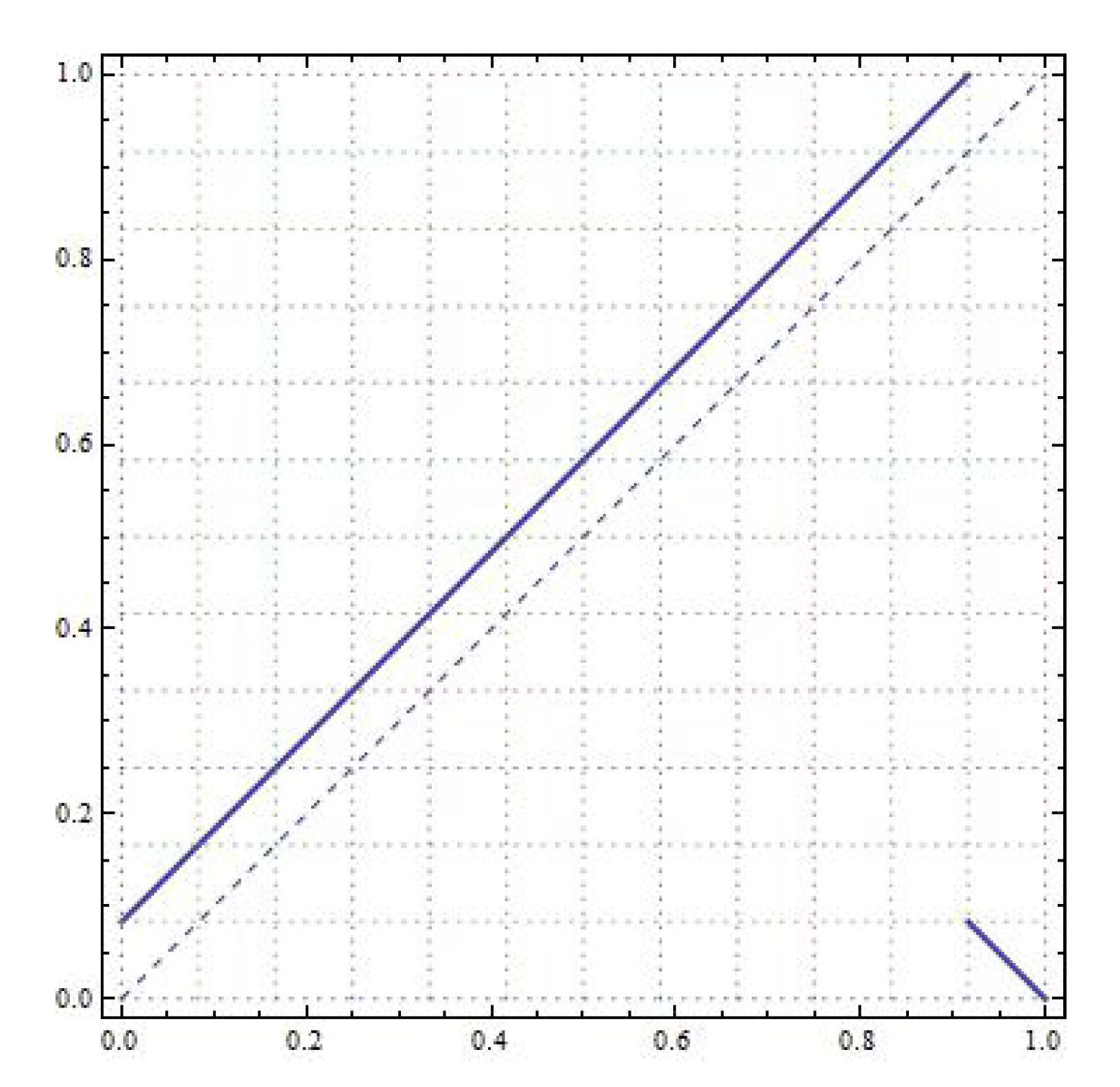
The shape of the map
T is shown in
Figure 16 for
and
. It is also shown the graph of the 2-IET with permutation
which is deeply connected with
T. First, we prove the next lemma.
Lemma 5. The 3-IET T has a fixed point if and only if .
Proof. Clearly T can have a fixed point in . Since such fixed point is , we easily see that it belongs to if and only if , which is equivalent to . □
Assume that
is a fixed point of
T, and therefore
. We take
and
. It is easy to see that
(respectively
) if and only if
(respectively
). We set
and
Observe that if
and hence
, then
and
. We define the interval
which is invariant by
T and contains the fixed point of
T. Then, we define
the 3-IET with permutation
and vector
. Note that, by construction,
cannot have fixed points, that is, either
or
. Then, we have the following result.
Proposition 3. Under the above notation, .
Proof. Note that all the points of J are periodic with period one or two. The proof follows taking into account that is invariant by T. □
Once we have analyzed the case in which
T has fixed points, it remains to discuss two cases: (a)
; (b)
, which is equivalent to
. However, the 3-IETs with permutation
and length vectors
and
are conjugate (see
Table 3), and thus have the same periods. So, it suffices to study the case
. We start by proving the next result.
Theorem 18. Let for some .
- (a)
If for some , then .
- (b)
If for some , then .
Proof. Note that . We have that T maps the intervals into for . Thus, the restrictions are conjugate to the 2-IET with permutation and vector length . Applying Theorem 6 for (notice that ), we obtain the result. □
Next, we need to consider the case for some . For that, we denote by the 2-IET with permutation and length vector . Given and a subset , we define . Then, we prove the following.
Theorem 19. Let for some .
- (b)
If , then .
- (b)
If , then , where is the 2-IET with permutation and and length vector.
Proof. We denote by
the 2-IET with permutation
and length vector
. By Theorem 6, if we iterate with
, the interval
is periodic with period
and the interval
is periodic with period
n. Observe that
Hence, since
for
, we find that
and from
for
, we have that
(a) The condition is equivalent to and . Then is the identity, so . On the other hand, is , so . Since , the proof of (a) finishes.
(b) The condition
is equivalent to
, and thus
. So,
is
, so
. On the other hand, notice that
and thus
is the 2-IET with permutation
and length vector
. So, (b) follows. □
If
, then the situation is much more complicated. The set of periods cannot be obtained easily from the set of periods of some 2-IET. For instance, when
we show the set of periods of
T for several values of
in
Table 7. For instance, for
and
, we have that
and this set of periods cannot be obtained from a 2-IET because it has at most two periodic components.


