1. Introduction
Air pollution, closely related to economic and social development as well as ecological environment construction, is a global problem that destroys human living environments. In recent years, the Chinese government has attached great importance to the prevention and control of air pollution. The World Air Quality Report 2021 released by the Swiss company IQAir pointed out that air quality in China continued to improve in 2021. Compared to 2020,
concentrations decreased in 66% of Chinese cities [
1]. However, China still faces environmental challenges. Air pollution is mainly composed of harmful gases and particulate matter, which are released into the atmosphere by natural or human activities, and its concentration is far beyond the self-purification capacity of the atmosphere, resulting in changes in the composition of the atmosphere, endangering human health and living environments. Smog, as a seriously harmful air pollutant, has received growing attention. Severe smog levels pose a huge threat to China’s public health [
2,
3,
4,
5]. Short-term exposure to air pollution will cause cough, dyspnea, headache, fatigue and other phenomena, while long-term exposure to air pollution will lead to respiratory diseases, cardiovascular damage, nervous system damage and other diseases, and may even lead to birth defects and death [
6,
7,
8,
9]. Climate warming, sea-level rises, acid rain, the hole in the ozone layer and other particulate pollution directly highlight the environmental problems caused by air pollution, harming human survival and development. To improve air quality and human living environments, air pollution has become a key topic for researchers, and monitoring, assessment, prediction and prevention have become important research directions in the study of air pollution. Smog is also closely linked to China’s economic development [
10,
11,
12,
13]. It is necessary to make full use of multidimensional big data and give full play to the advantages of statistics and artificial intelligence technology. By virtue of interdisciplinary development, researchers have been able to vigorously develop statistical modeling theory and deep learning technology for accurate prediction and effective control of urban air quality. As a result, a solid theoretical foundation and effective technical support can be provided for improving the capabilities and level of ecological and environmental conservation.
Fine particulate matter (
) is the most common object in the studies of pollutant concentration, and the higher the concentration in the air, the more serious the air pollution [
14,
15,
16]. From a statistical point of view, pollutant concentration prediction has become an important research direction in air pollution forecasting and prevention. The existing research on air pollutant concentration mainly focuses on the sources, concentration distributions, fluctuations, affecting factors, adverse effects on human health and so on. Quantitative prediction of pollutant concentration is the most common statistical method for dealing with air pollution problems, and multivariate regression, cluster analysis and principal component analysis are the most frequently used statistical models. Chen Songxi, an academician of the Chinese Academy of Sciences, applied non-parametric statistics to the national air pollution assessment and prevention research and proposed a method for adjusting spatio-temporal meteorological factors to remove the meteorological confounding effect in atmospheric environmental monitoring, providing a scientific method for accurately measuring pollutant discharge and evaluating air pollution control [
17,
18,
19,
20,
21,
22]. Wang et al. (2020) [
23] established a spatio-temporal
pollution land use regression (LUR) model suitable for large cities based on parametric, non-parametric and semi-parametric classical statistical algorithms combined with meteorological factors, with the ability to monitor
concentration with high spatio-temporal resolution.
In order to improve the prediction accuracy, classical extreme value theory (EVT) has attracted more and more attention. Compared with fine weather, researchers are more concerned with observations of pollutant concentrations exceeding a certain high threshold. Pickands (1975) [
24] pointed out that observations above a certain threshold can be approximated well by the generalized Pareto distribution (GPD). As a branch of EVT, GPD plays an important role in many fields. In the field of hydrometeorology, the GPD model is used to analyze and forecast natural phenomena such as floods, wind and rainfall [
25,
26]. In the financial field, stock yield is non-normal and thick-tailed, which can be well fitted by a GPD [
27,
28]. In the field of insurance, insurance losses are generally non-negative with a thick tail, and a GPD is usually used to predict the maximum loss [
29,
30].
Due to the strong time correlation of observations, a traditional model with fixed parameters cannot perfectly fit the time-series observations in reality. To solve this problem, many researchers have conducted in-depth research on the dynamic extreme value distribution model and the dynamic over-threshold GPD model. Using the autoregressive mechanism of the GARCH model, Zhao et al. (2018) [
31] established an autoregressive conditional Fréchet model with time-dependent parameters (type II GEV) for the sequence of daily maximum stock returns. They solved the maximum likelihood estimation of the model parameters and studied the large-sample properties of the parameters. Chavez-Demoulin et al. (2014) [
32] applied a Bayesian method to update the time-varying GPD parameters for the UBS stock price, which was a non-parametric method applied to a POT–GPD model. Kelly and Jiang (2014) [
33] built a dynamic tail model with POT–GDP for panel data and measured the tail risk of the S&P 500 index. Massacci (2017) [
34] studied the time-dependent dynamic parameter estimation of a GPD through the score-based approach, in order to accurately estimate the tail index from U.S. size-sorted decile stock portfolios. Shen et al. (2020) [
27] established an autoregressive conditional Pareto (ACP) distribution model via an exponential function. The maximum likelihood estimation of the parameter was given, and its properties were studied. Based on the parameter estimation, they employed the ACP model to the Dow Jones Industrial Average and the S&P 500 index. Deng et al. (2020) [
35] applied a dynamic model to air quality management, taking time and meteorological factors into consideration and establishing a dynamic conditional autoregressive Weibull distribution model (type III GEV) via the maximum daily pollutant concentrations. The probabilistic properties of the autoregressive model were investigated in their study. As is well known, it is difficult to fit the
time series accurately, so the model selection and statistical inferences are the most important and common challenges for real data applications.
Threshold selection is a critical issue for fitting the autoregressive conditional generalized Pareto distribution model. In practice, the threshold should be chosen in advance. If the threshold is too large, the sample size of observations exceeding the threshold will be too small, which may increase the variance of the parameter estimation and affect the estimation effect. If the threshold is too small, the sample size can be increased, but the estimator is prone to bias. Choulakian and Stephens (2001) [
36] transformed the threshold selection into the goodness-of-fit test of the model. Through the selection method, an appropriate threshold was chosen, allowing the exceedance to follow the GPD, and the threshold selection was carried out at the same time as testing the model. Bermudez et al. (2001) [
37] used a Bayesian predictive approach to the peaks-over-threshold (POT) method, which can also be applied to small-sample situations. Bader et al. (2018) [
38] proposed an automated threshold selection procedure based on a sequence of goodness-of-fit tests, and attained automatic threshold selection by applying stopping rules, which transform the results of ordered, sequentially tested hypotheses to control the false discovery rate. Yang et al. (2018) [
39] developed an empirical threshold selection method based on the relationship between eigenvalues and thresholds. Schneider et al. (2021) [
40] proposed selecting the threshold by minimizing the asymptotic mean squared error of the Hill estimator.
With the continuous development of artificial intelligence and machine learning, an increasing number of scholars have applied traditional machine learning methods to statistical prediction models in recent years and achieved good results in terms of accuracy and time efficiency. Boznar et al. (1993) [
41] compared prediction results based on the three-layer neural network perceptron with the results generated by a traditional atmospheric diffusion model. Neagu et al. (2002) [
42] used a fuzzy neural network model to predict the concentration of nitrogen oxide pollutants, achieving good results. Esfandani and Nematzadeh (2016) [
43] proposed a prediction model for air quality in Tehran based on a feedback neural network. Amarpuri et al. (2019) [
44] established a convolutional long short-term memory network to predict carbon dioxide emissions and achieved ideal results. An air pollution prediction model based on LSTM is a good choice for predicting
concentrations. García et al. (2020) [
45] analyzed the concentrations of nitrogen dioxide (
), nitrogen oxides (
), particulate matter (
) and toluene (
) at eight sites in Madrid (Spain) through seven regression-based machine learning models and time-series models. Sánchez-Pérez et al. (2020) [
46] established a complete spatio-temporal dispersion model for pollutants through a network simulation method, to obtain the concentrations of pollutants released at any time in a given space. Sayeed et al. (2021) [
47] used a generalized deep convolutional neural network (CNN) model to predict air pollutants, which could predict the hourly pollutant concentration within 7 days with relatively high accuracy.
In this paper, dynamic autoregressive mechanisms are applied, and weather and air quality factors are also involved in our model. The framework of this paper follows that of [
27]. The three main contributions of this paper are as follows. First, we construct a dynamic conditional generalized Pareto distribution (DCP) with both weather and air quality factors to fit the smog observations, considering the time-dependency of the scale parameter and the tail index of the GPD. Secondly, the threshold is chosen using a threshold selection program rather than by specifying a quantile. Thirdly, the
time series are predicted by combining the DCP model with deep learning technology.
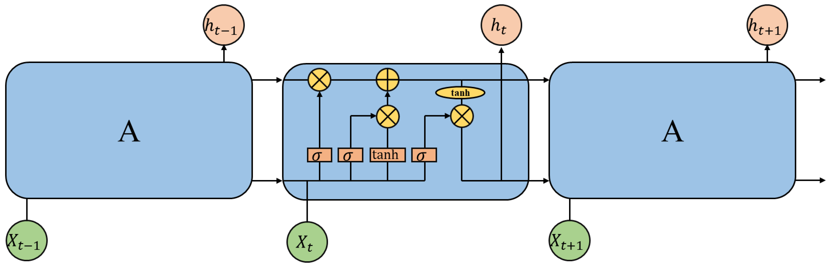
4. Long Short-Term Memory Model
The main purpose of LSTM is to solve the problem of long-distance dependency in the training of recurrent neural networks. First, it is necessary to set the cell memory unit, and introduce the forget gate, input gate and output gate into the recurrent neural network (RNN), so that information transmission can be controlled. The state (namely the memory unit) update is also based on these “gates”, which ensure that the LSTM model can save long-distance information. Under the influence of the memory unit, these “gates” will be in a controllable range. LSTM then can save, update and read long-distance information, and gradient explosion or disappearance during training are well solved. In the time-series data for air pollution, more comprehensive long-distance dependence information can be extracted. From the perspective of the whole model, the main components are as follows: output gate
, input gate
, memory unit
and forget gate
. The structure is shown in
Figure 1.
The first “gate” that the LSTM passes through is the “forget gate”, which discards part of the information in the previous memory unit. This step is realized by a sigmoid function, which uses the weighted values of the current input and the output of the previous moment to obtain a number in the range of 0–1, which controls the information transfer. The value 1 represents complete retention and 0 represents complete discarding. The details are given in Equation (
17):
The input gate controls what information is added to the cell, and the calculation process is shown in Equations (
18) and (
19):
The output gate controls what information is used for the task output at this moment, and the calculation process is shown in (
20) and (
21):
In the above equations, , and denote the weight matrices of the corresponding gate, , and denote the corresponding gate bias matrices, and tanh denote the activation functions, denotes the output gate, denotes the input gate, denotes the memory unit, denotes the forget gate, denotes the input at time t and denotes the output at time t.
5. Simulation Study
In this section, the performance of the MLE for the DCP models is investigated using six numerical experiments. To investigate the performance of the MLE, we generate data from the three DCP models given in (
5) and (
8)–(
13), with the parameters shown in
Table 1. These sets of parameters are the MLEs obtained from an analysis of real observations in Beijing from 3 January 2015 to 8 August 2020 and from 1 January 2018 to 8 August 2020, where the weather factors are from the China Meteorological Data Service Center and the air quality factors are from the China National Environmental Monitoring Center. In addition, the estimations of
and
are close to 0, especially in the three models from 3 January 2015 to 8 August 2020, which indicates that the scale parameter
can be considered a constant to a certain extent (a consideration that will be realized in future research). Due to more attention being given to the tail index
and the wider applicability of the DCP models, we made no changes to
.
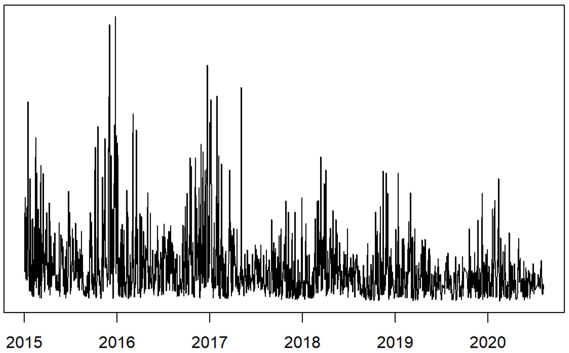
Figure 2 displays a line graph of the
concentration time series in Beijing. As shown in
Figure 2, with the improvement in the national environmental governance level and public awareness of environmental protection, the
concentration generally shows a downward trend.
Figure 2 shows that 2018 is a noteworthy year with significant governance effects, suggesting that
concentrations after this need to be analyzed separately. Hence, real data from 1 January 2018 to 8 August 2020 are also fitted to the three DCP models, in addition to the real data from 3 January 2015 to 8 August 2020. According to the World Air Quality Report 2021 released by IQAir [
1], China has seen a 21% overall reduction in annual
concentrations since 2018, which justifies the separation of the data from 1 January 2018 to 8 August 2020.
Threshold selection is a key issue in extreme value analysis based on the POT method. For these two sets of observations, from 3 January 2015 to 8 August 2020 and 1 January 2018 to 8 August 2020, we select two thresholds determined by Bader et al. (2018) [
38] and Davison and Smith (1990) [
50]. Bader et al. (2018) [
38] proposed an automated threshold selection procedure using a stop rule that controls the false discovery rate in ordered hypothesis testing. The ForwardStop rule provides an automated selection procedure combined with sequential hypothesis testing when the level of desired error control and a set of thresholds are given. Based on the goodness-of-fit of the GPD, Davison and Smith (1990) [
50] proposed a threshold selection approach where the threshold is chosen as the lowest value above which the GPD fits the exceedances adequately. In this study, the threshold selection results were 2.4660 using the method of Bader et al. (2018) [
38] for
data from 3 January 2015 to 8 August 2020 and 0.5716 using the method of Davison and Smith (1990) for
data from 1 January 2018 to 8 August 2020, and approximately
and
of the corresponding real data exceeded these two thresholds, respectively, ensuring a sufficiently high value.
Table 2,
Table 3,
Table 4,
Table 5,
Table 6 and
Table 7 show the averages of the mean values and the standard deviations with different sample sizes from the three DCP models in the above two periods. We also calculated the corresponding root mean squared error (RMSE) and absolute bias (Abias) to measure the estimation effect, as shown in
Table 2,
Table 3,
Table 4,
Table 5,
Table 6 and
Table 7. We obtained simulated exceedances
with lengths of 1000 and 2000, respectively. The experiments were repeated 500 times for each sample size. As shown in
Table 2,
Table 3,
Table 4,
Table 5,
Table 6 and
Table 7, the RMSE and Abias values for the parameter estimations using the real data from 1 January 2018 to 8 August 2020 were mostly smaller than those from 3 January 2015 to 8 August 2020, while those for the sample size of 2000 were mostly smaller than those for the sample size of 1000, and the parameter estimation of the tail index
was better than that of
. The values of RMSE and Abias explain the validity of our estimation.
To enable observation of the performance of our model more directly,
Figure 3 depicts the dynamics of the tail index
estimated by MLE (red line) and the simulated tail index
(black line) under the experiments for
n = 2000. We can see that the estimated tail index
was almost the same as the simulated tail index
in the three DCP models. In addition, we calculated the correlation between the two series, and the results were 0.9328, 0.9559, 0.9921, 0.9964, 0.9591 and 0.9679, corresponding to
Figure 3a–f, respectively, which shows the similarity of the two curves better. However, we cannot judge the simulation effect from the similarity of the two curves only.
Figure 3 illustrates the sufficiency of our estimation.
6. Real Data Applications
In this section, to verify the performance of the DCP models, we consider the weather and air quality time series in Beijing from 3 January 2015 to 8 August 2020 and from 1 January 2018 to 8 August 2020 obtained from the China Meteorological Data Service Center and China National Environmental Monitoring Center, as the sample for our experimental analysis. Based on these two periods observations, we employed the three DCP models (one with weather factors, one with air quality factors and the last with mixed weather and air quality factors) given in Equations (
5) and (
8)–(
13) to fit the smog data and used the MLE method described in
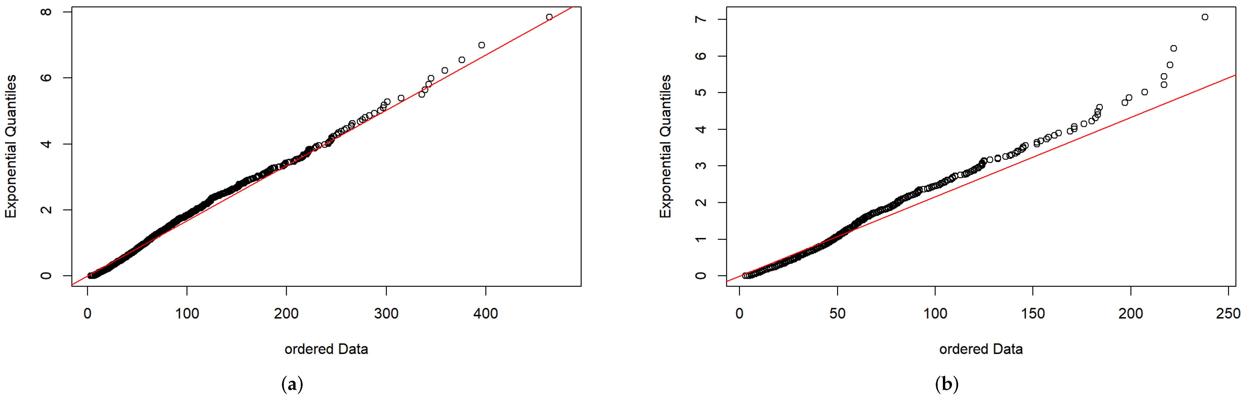
Section 3 to estimate the parameters. In both cases, the DCP models showed their superiority in reflecting the time dependence of the pollutant concentration, providing a potential warning signal for smog prevention and control. First, we made a fat-tailed diagnosis of the observations using an exponential QQ plot.
Figure 4 shows that the real data for
in Beijing from 3 January 2015 to 8 August 2020 and from 1 January 2018 to 8 August 2020 are fat tailed.
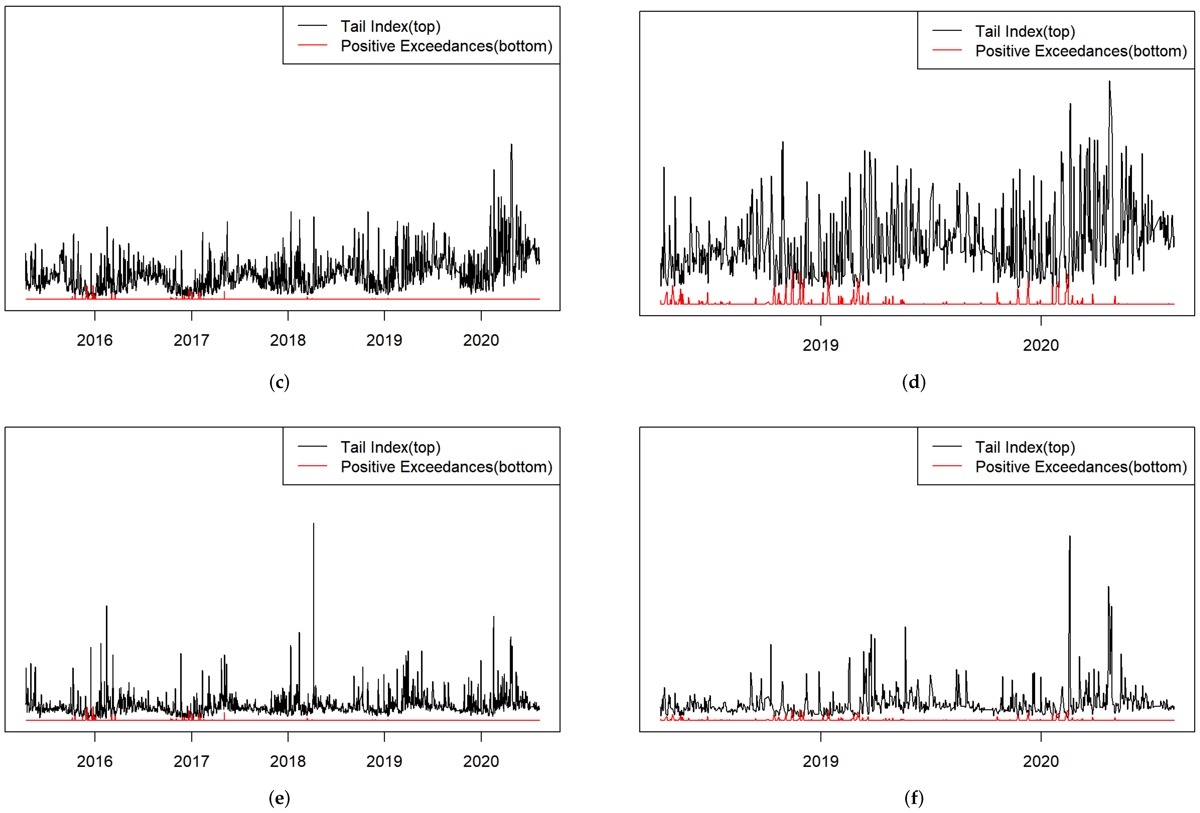
From the results in
Table 1, we can see that the tail index
is more affected by
, which is consistent with
Figure 5. The estimated tail index of the DCP can reflect the severity of smog to some extent and may even play an early warning role for smog disruption. The graph of the estimated tail index
and positive exceedances
from the three DCP models is given in
Figure 5, which shows that there is a strong negative correlation between
and
, and the tail index volatility is more intuitive. It is interesting to note that
Figure 5a,c,e and
Figure 5b,d,f have very similar variation tendencies, and it can clearly be seen that the tail index
starts to decline in the middle of each year, and at the end of the year the tail index becomes lower, which can be regarded as an effective indicator for measuring the level of smog.
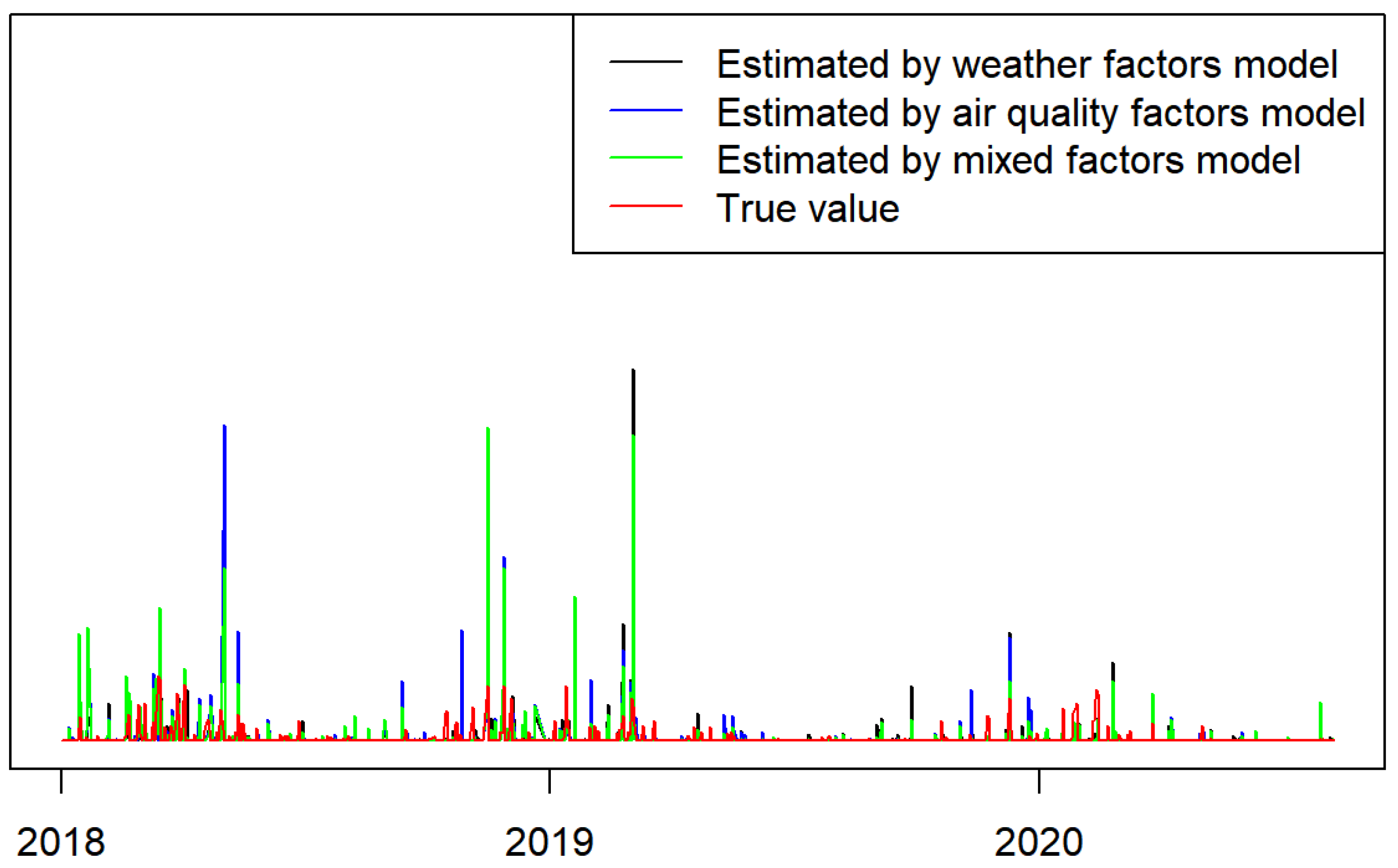
Using the estimated parameters given in
Table 1, we generated a sequence of fitted
values based on Equation (
5) and plotted the line graphs of the fitted
values and real exceedances
during the period from 1 January 2018 to 8 August 2020, as shown in
Figure 6. It can be seen that the true values
and the estimated values
from the three models were almost consistent in trend, and the three models were more sensitive to the estimation of
, but the model with mixed weather factors and air quality factors showed values closest to the true values, which also verifies the superiority of the mixed model over the other two models and is consistent with the conclusion mentioned in
Section 5. A comparison between the fitted
and real
exceedances during the period from 3 January 2015 to 8 August 2020 was also performed, and similar results were obtained. Due to limited space, only
Figure 6 is shown.
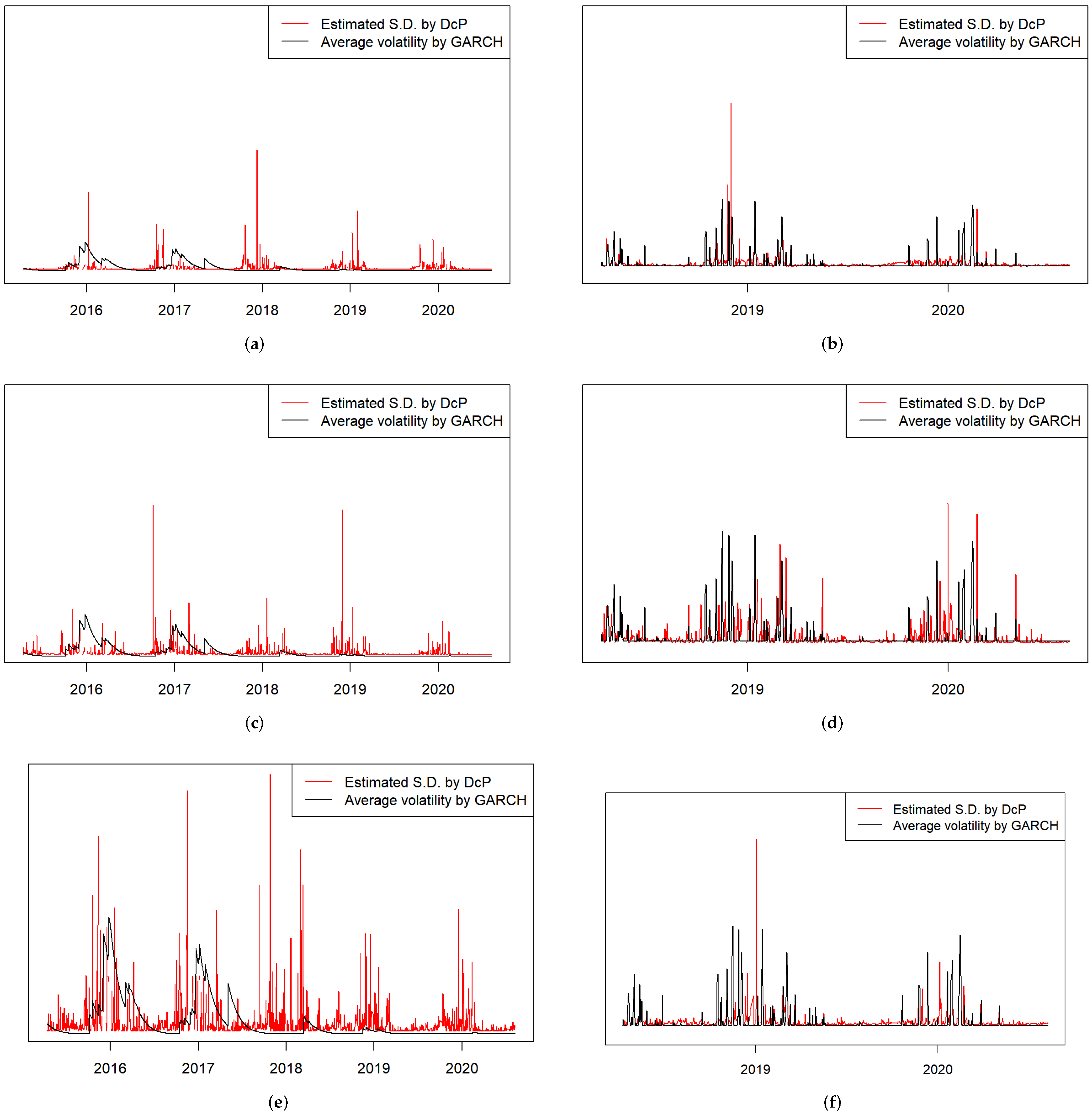
Next, we compared the estimated variances from the DCP models and GARCH, as shown in
Figure 7. Similarly to [
27], we calculated the conditional variance
Figure 7 shows that the standard deviations given by the DCP models and GARCH had similar trends, indicating that the DCP models could accurately reflect the volatility in a sense. Compared to the estimated volatility of GARCH, the DCP models are more sensitive in smog instances, thus potentially playing a better role in early warning. This is clearest in
Figure 7e, where the fluctuation is largest.
We computed AIC and BIC from the DCP and dynamic conditional Weibull (DCW) model given in [
35]. The results are presented in
Table 8. As shown in
Table 8, the DCP model is more suitable than the DCW model, based on AIC and BIC criteria.
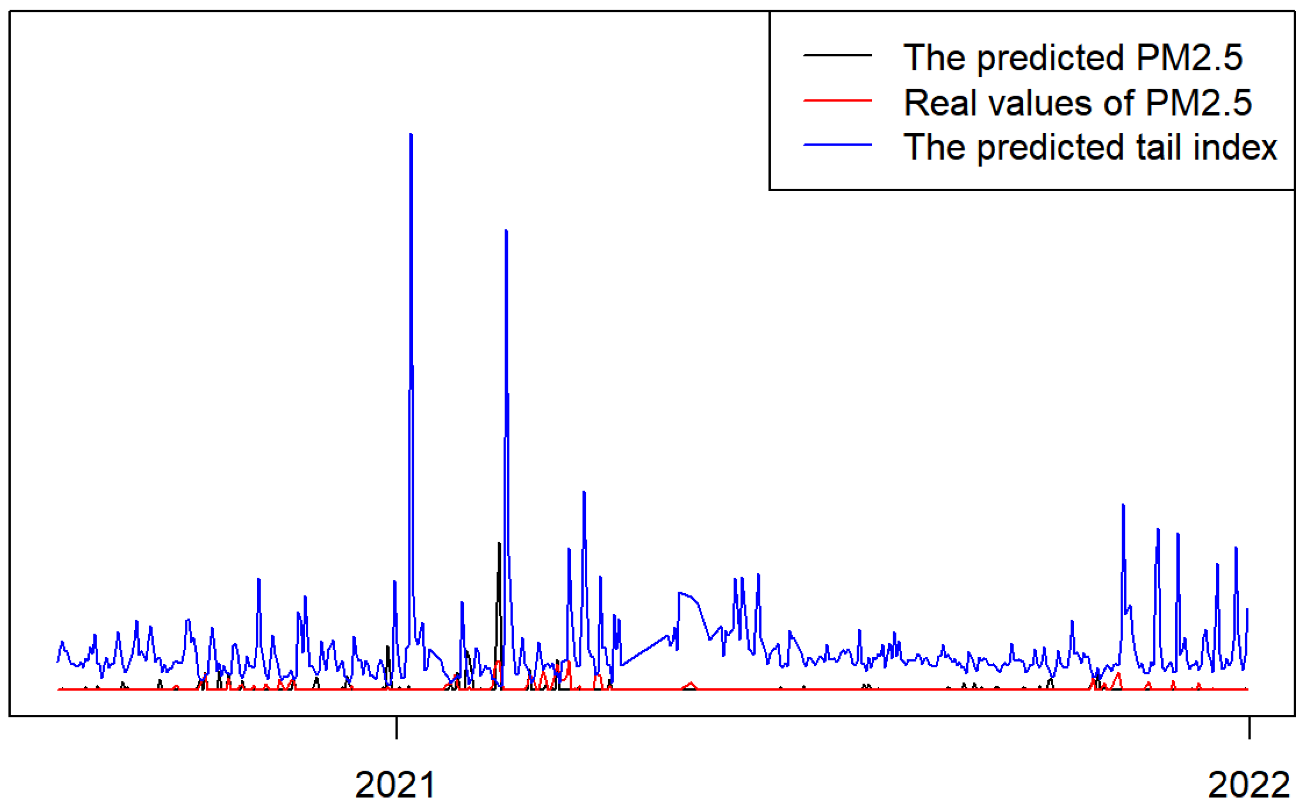
Finally, we used our proposed three models (
5) and (
8)–(
13) to predict the daily PM
2.5 values from 9 August 2020 to 31 December 2021. We present only the results for the mixed models in (
5), (
12) and (
13) here, with a training sample from 1 January 2018 to 8 August 2020, since similar results were obtained from the three models. The tail index
given in (
13) and PM
2.5 given in (
5) were predicted by using the real weather and air quality factors and the parameter estimation results given in
Table 1. In order to analyze the fluctuating tendency and correlations of
and PM
2.5, the prediction results are presented together in
Figure 8. From
Figure 8, we can see that there is a strong negative correlation between
and PM
2.5, which enables the tail index to be used as a warning signal for air pollution. Furthermore, compared with the real smog values, the predictability of the future variation of PM
2.5 performs relatively well, as the real and predicted values are relative close and have a similar tendency.
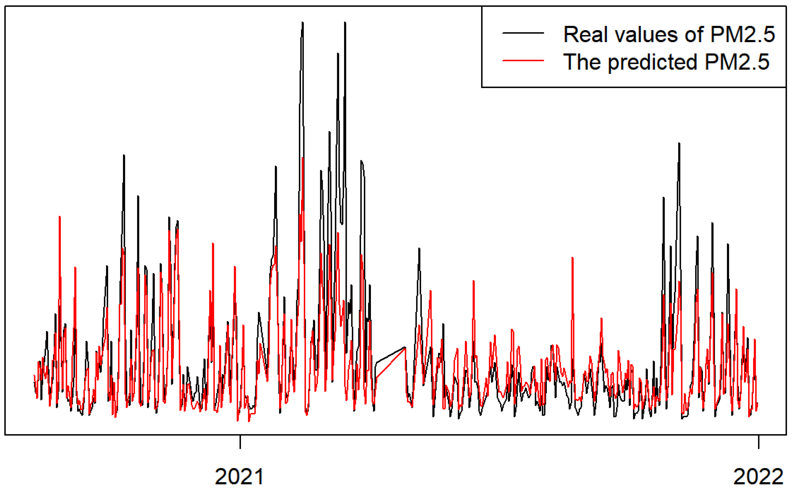
In addition, we used weather and air quality factors (including
) with the LSTM technique to predict daily PM
2.5 values.
The air pollution data from 1 January 2015 to 25 November 2019 were used as training data, those from 26 November 2019 to 8 August 2020 were used as verification data and those from 9 August 2020 to 31 December 2021 were used as test data.
The LSTM network was trained by using the weather, air quality factors and
time series in Beijing to construct a training set. Then, various weather and air quality factors were input into the test set to predict the
from 9 August 2020 to 31 December 2021 over a long period. As shown in
Figure 9, the trend of the prediction for
was accurate, especially when the true values of
were less than 100.
To better evaluate the experimental results quantitatively, the RMSE and coefficient of determination (
) were calculated, and the results were 20.14 and 0.65, respectively.
7. Conclusions
In this paper, we investigated the prediction of pollutant concentrations using statistical inference methods and deep learning techniques. On the one hand, we proposed three models combined with the autoregressive structure under the POT framework. After obtaining two sufficiently high thresholds selected using the methods of by Bader et al. (2018) [
38] and Davison and Smith (1990) [
50], the DCP models provided a direct dynamic modeling of exceedances in the
time series, such that the scale parameter and tail index of the conditional generalized Pareto distribution changed over time. Weather and air quality factors were added to the DCP models for better performance and higher efficiency. The maximum likelihood estimation method was introduced to estimate the parameters in the DCP models, and its asymptotic properties were investigated. Simulation studies were carried out to demonstrate the validity and sufficiency of the estimation, revealing that the parameter estimation of the DCP models was not sufficiently accurate but the tail index dynamics could be well approximated in the DCP models. Real data applications were used to present the superiority of the DCP models, showing that they could shed new light on the prevention and control of smog. On the other hand, based on the factors used in the mixed DCP model, we used LSTM to study the prediction of pollutant concentrations, and achieved satisfactory results. This paper aimed to improve the prediction ability for the concentration of pollutants, and valuable results were achieved. Given the requirements of the air pollution control target for further promoting ecological and environmental protection in the next five years, the proposed approaches and results in our paper are useful. To some extent, they could provide a theoretical basis and effective tools for improving the national air quality forecasting system, thus benefiting public health.
Nevertheless, there are still some points to be considered. In the DCP model with the autoregressive structure, it is meaningful to add weather and air quality factors, enriching the model and making it consistent, stable and sensitive. However, the relationship between the factors has not been scrutinized carefully, resulting in a lack of attention to its impacts on the model. In addition, it is possible to obtain better results when we compare other estimation methods. Therefore, prediction, as an important direction in our study of air pollutant concentrations, still has a long way to go. Combining artificial intelligence and machine learning, the prediction accuracy will certainly be improved by using a forecast combination, synthesizing the methods used to obtain the estimated results. Finally, with the help of combination forecasting, the advantages of individual forecasts are retained, and effective information is fully utilized to comprehensively forecast air pollution. In this work, we strive to make valuable advances in the intersection of statistics and machine learning and to provide effective theoretical and technical support for national continuous improvement of the modernization level of ecological environmental governance.


