
The Generalized Alpha Exponent Power Family of Distributions: Properties and Applications


Abstract
:1. Introduction
- (i)
- ;
- (ii)
- is monotonically increasing and differentiable; and
- (iii)
- ⟹ and ⟹.
- (i)
- Constructing new G-families as a function of a CDF, .
- (ii)
- The proposed extension of the APT is based on a generator instead of the existing generator .
- (iii)
- The proposed generator has the power to produce better results of estimates and goodness of fit tests that can make it attractive and distinguishable for applied researchers.
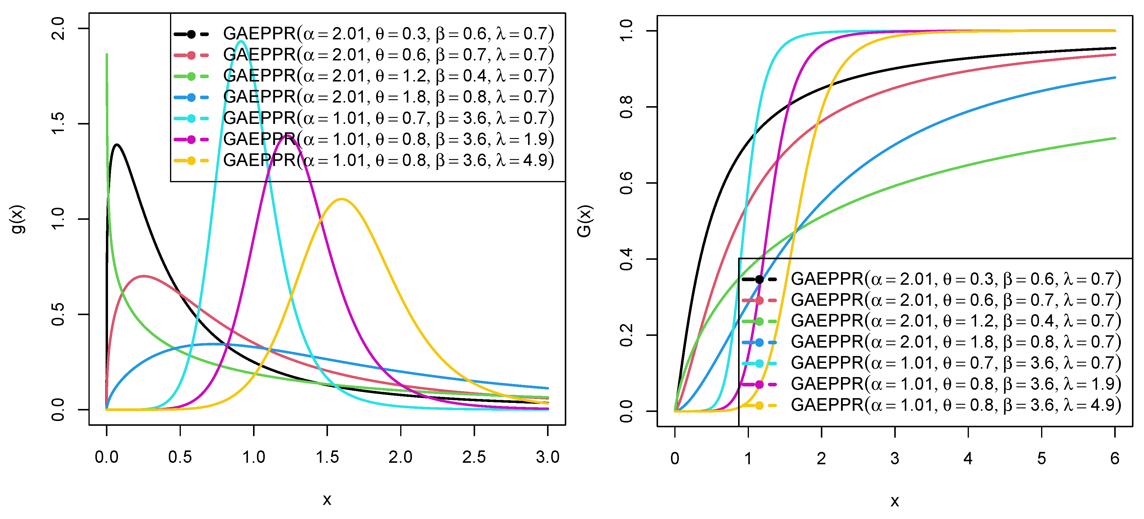
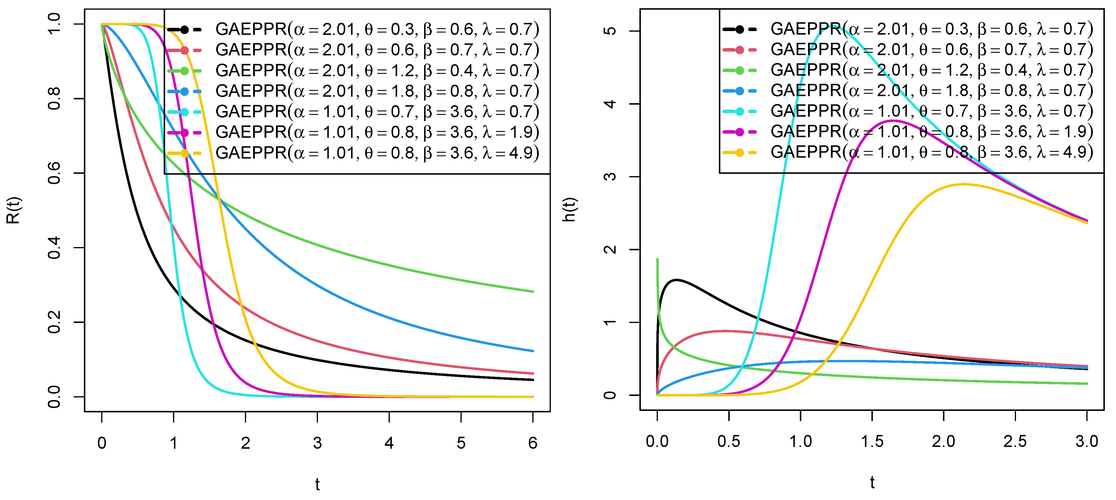
2. The Generalized Alpha Exponent Power Power Rayleigh Distribution (GAEPPRD)
3. Statistical Properties
3.1. Moments
3.2. Moment Generating Function (MGF)
3.3. Mode
3.4. Quantile Function (QF)
3.5. Skewness and Kurtosis Using Quantile Approach
3.6. The Mean Deviation (MD)
3.7. Rényi Entropy (RE)
3.8. The Probability Weighted Moments (PWMs)
3.9. Distribution of Order Statistic (OS)
4. Maximum Likelihood (ML) Estimation
Asymptotic Confidence Bounds (ACBs) of GAEPPRD
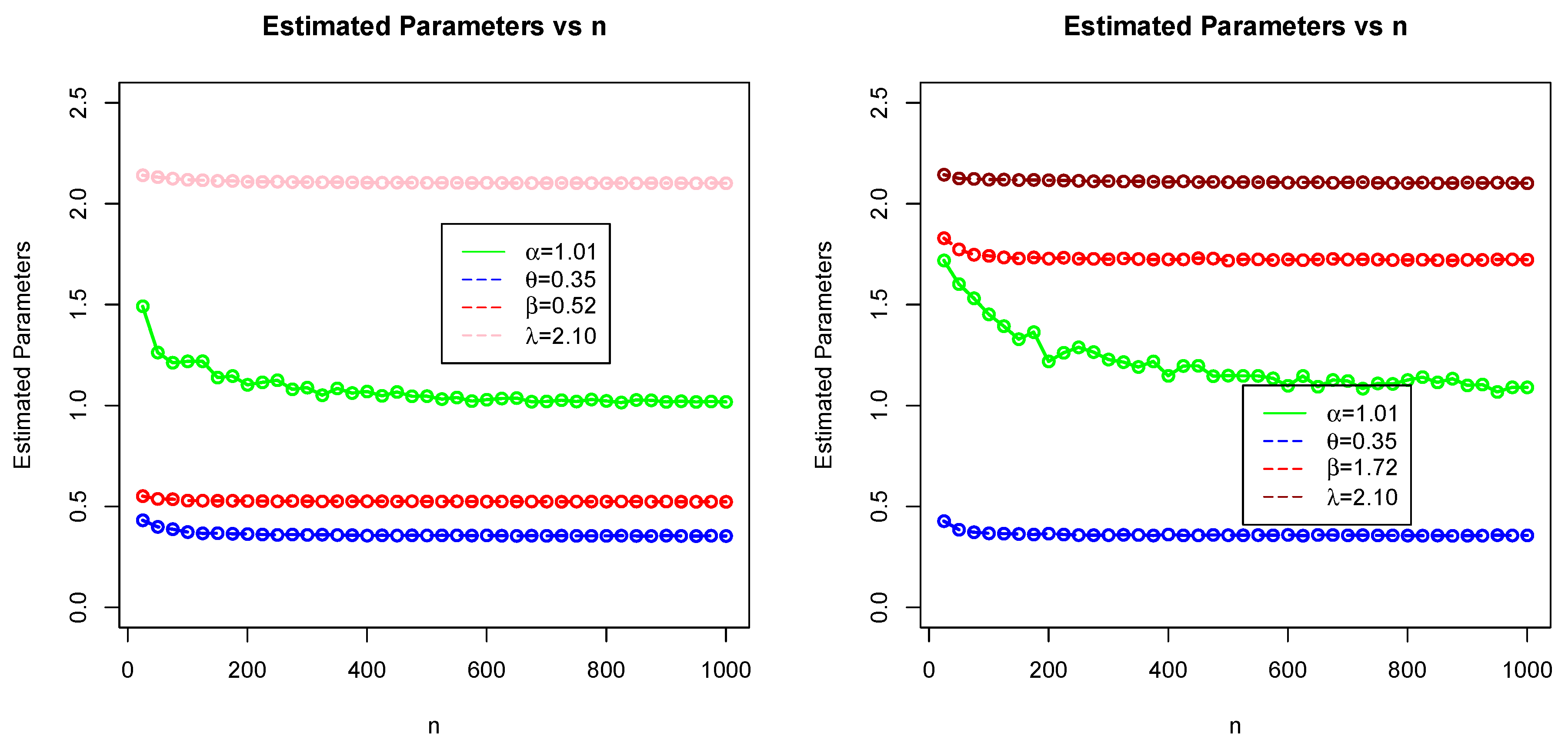
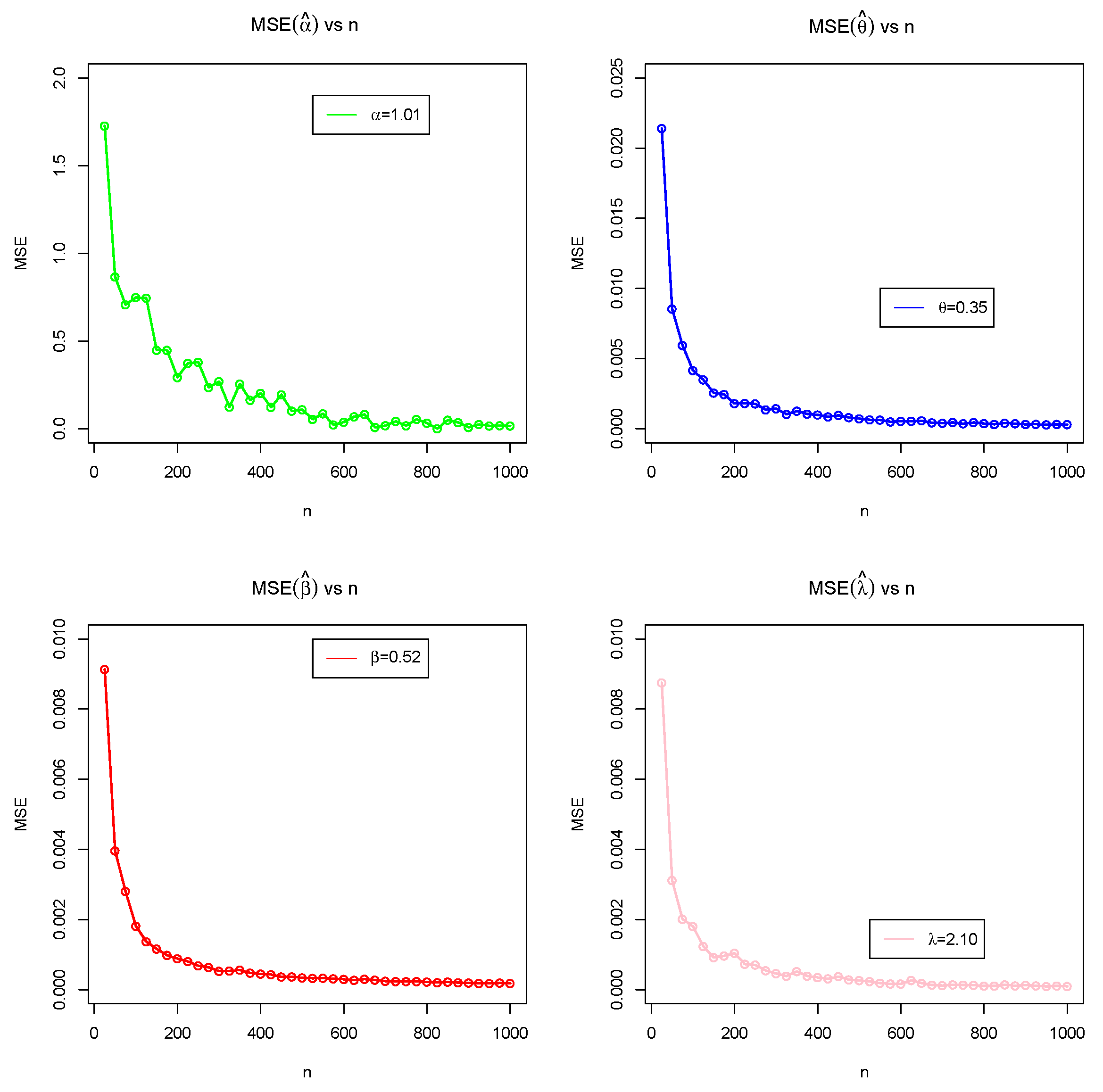
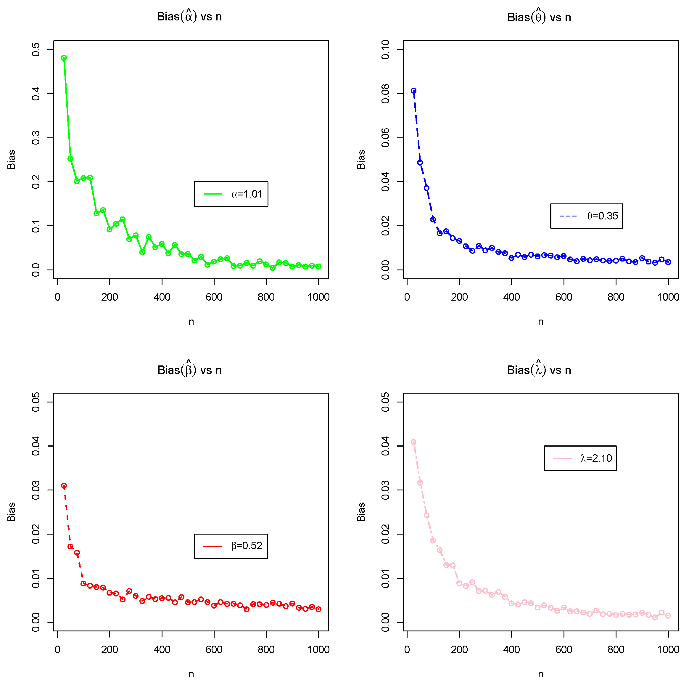
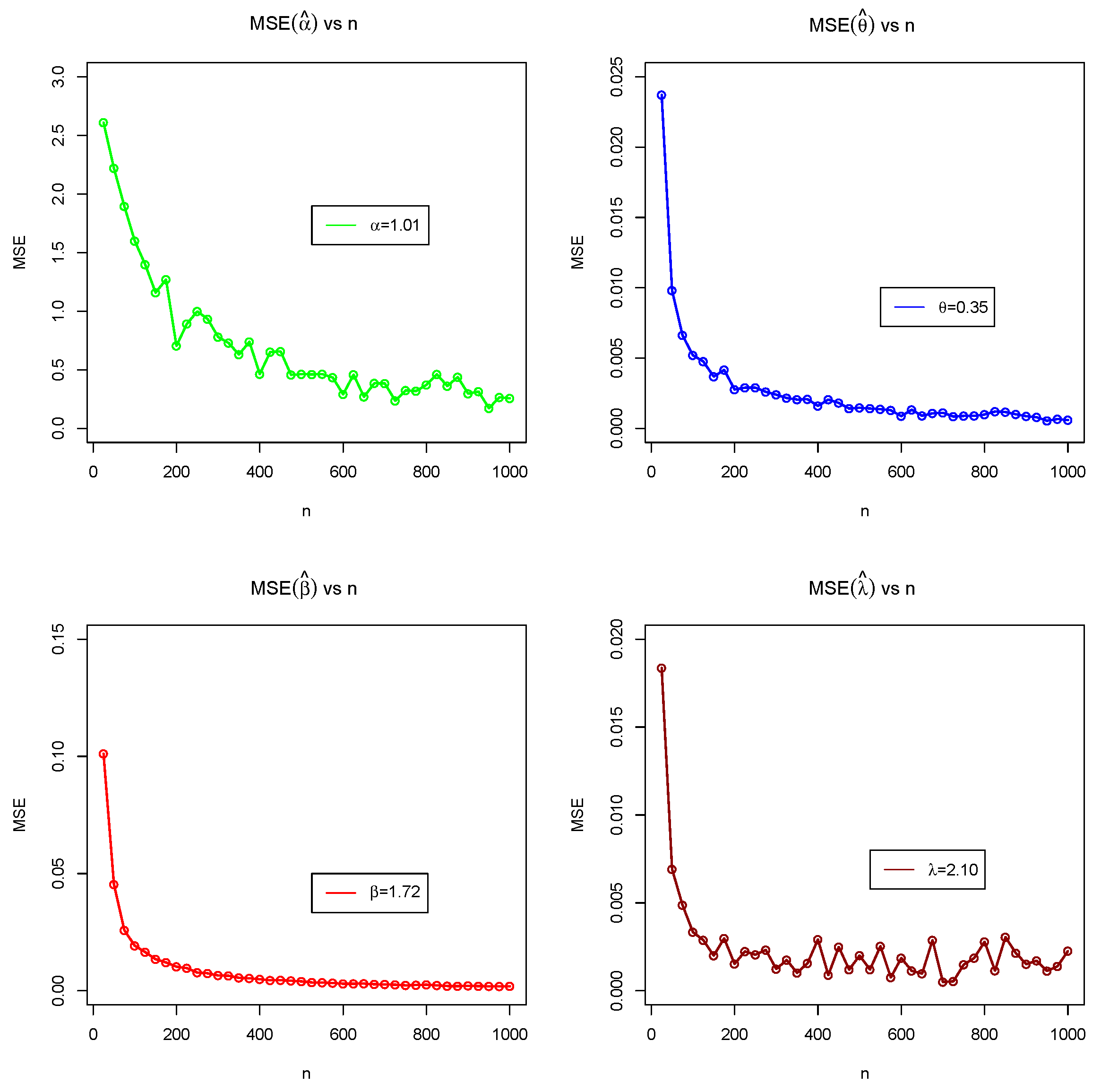
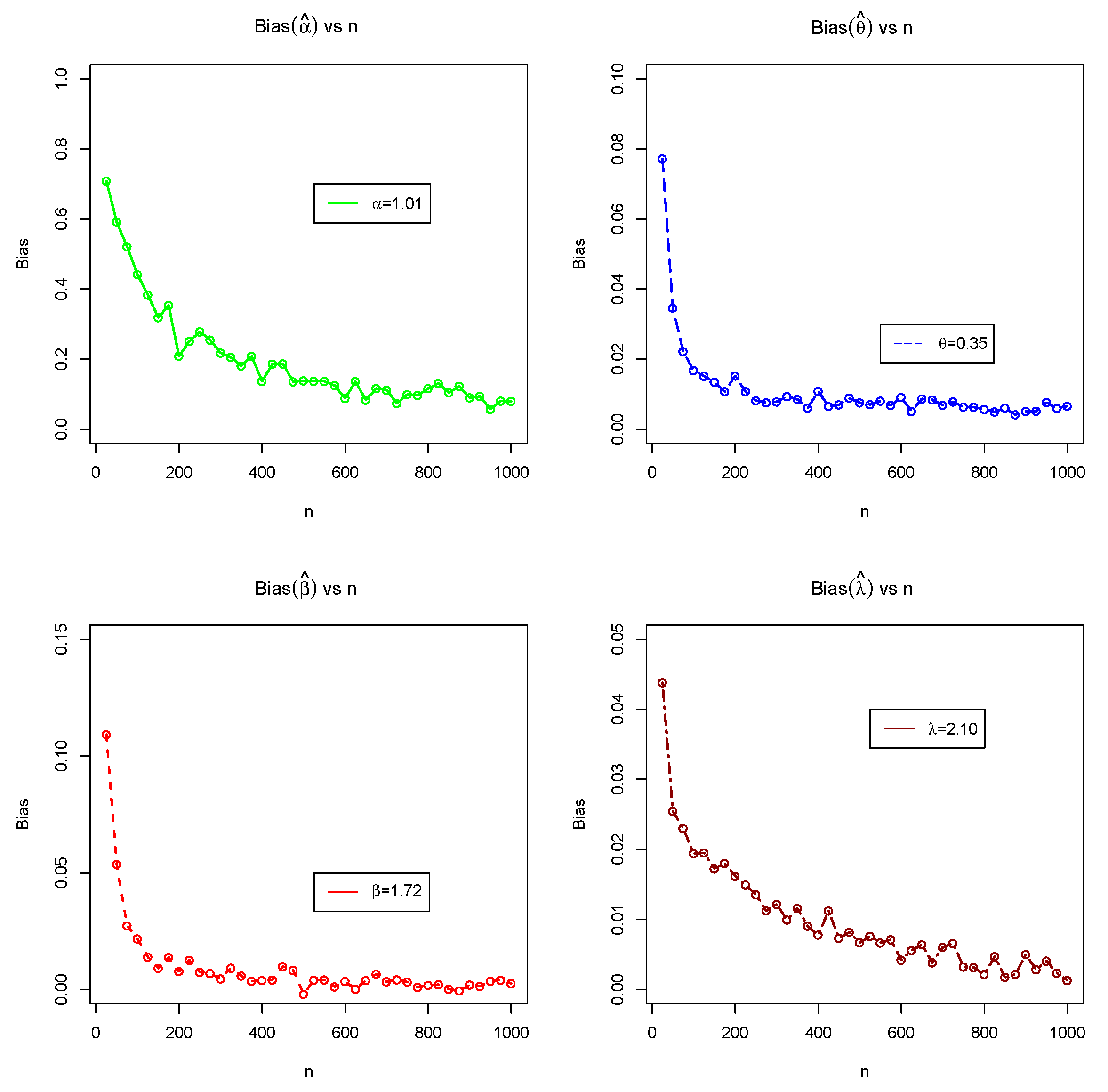
5. Monte Carlo Simulation Study (MCSS)
- MSE and biases decrease as n increases.
- Estimates of GAEPPRD are very steady and are nearer to the true value of parameters as n increases.
6. Applications
- Akaike information criterion (IC)
- Bayesian IC
- The Hannan–Quinn IC
- Consistent AIC
- Test statistics: Anderson–Darling (AD)
- Test statistics: Cramér–von Mises (CM)where is LLF at MLEs, q (no. of model parameters), n (sample size), and (calculated value at the position in the sample point according to ascending order).
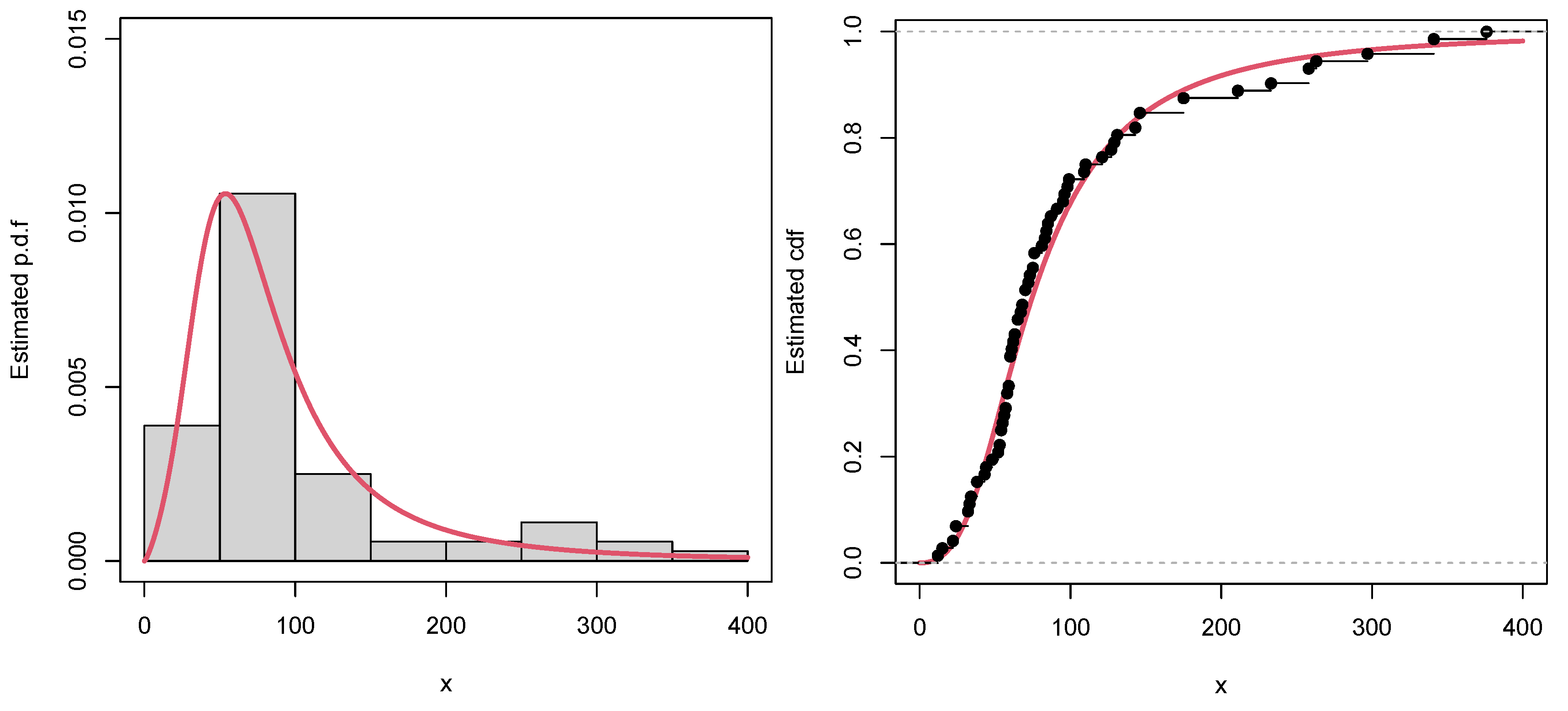
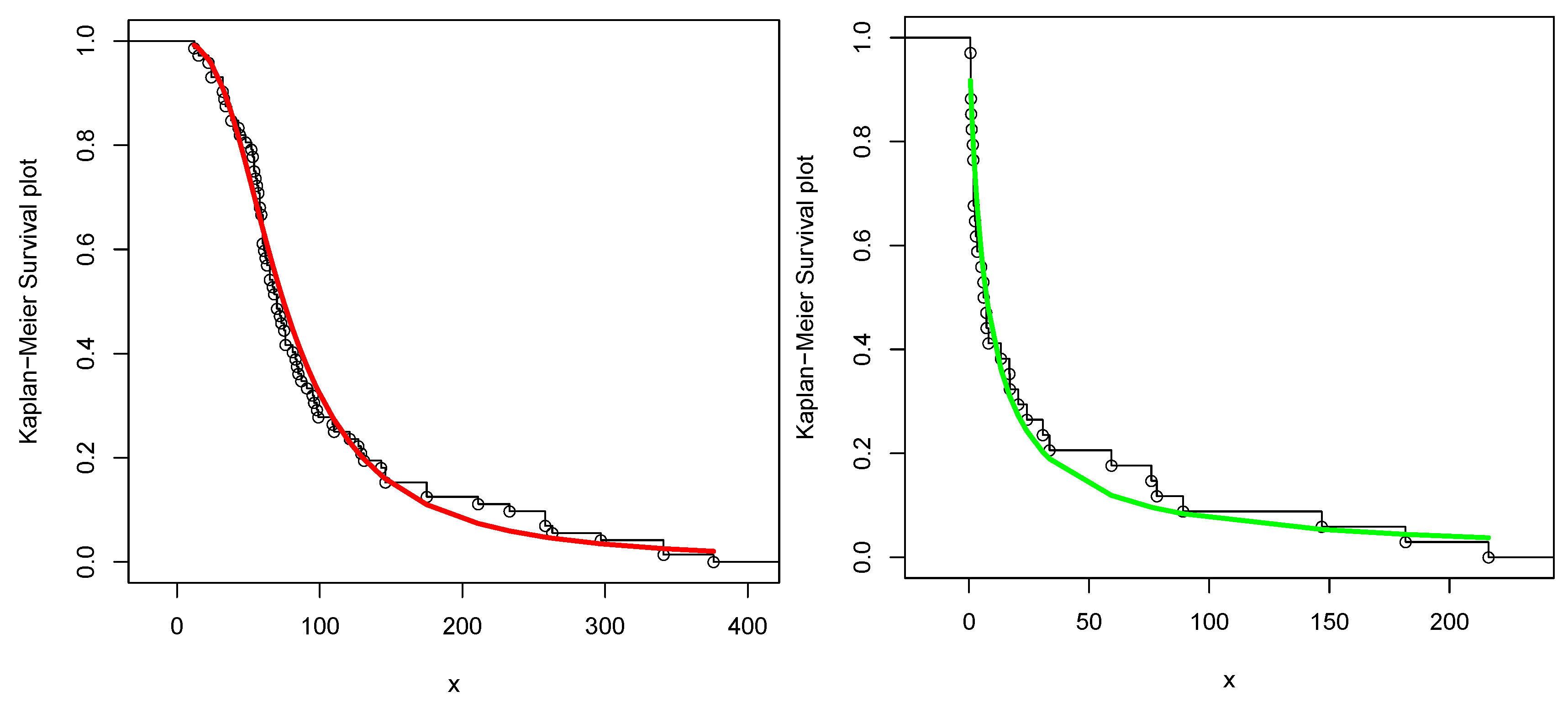
6.1. Dataset 1
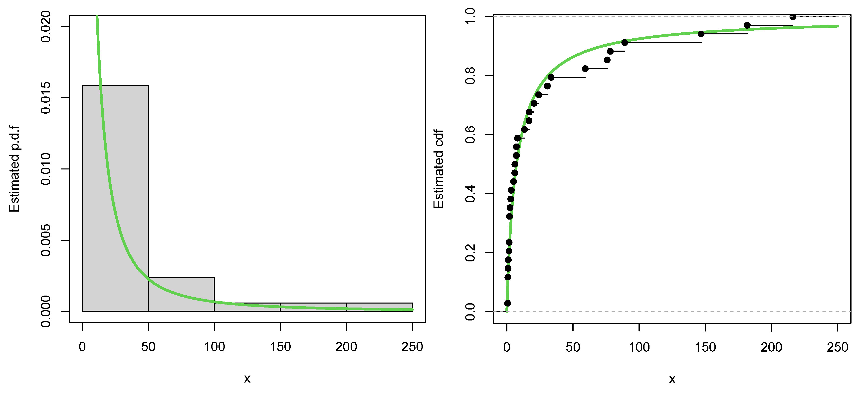
6.2. Dataset 2
- The RD
- The APR distribution
- The exponential distribution
- The APE distribution
- The EIR distribution
- The APEIR distribution
- The Gumbel distribution
- The APG distribution
6.3. Illustration
7. Conclusions
Author Contributions
Funding
Institutional Review Board Statement
Informed Consent Statement
Data Availability Statement
Acknowledgments
Conflicts of Interest
References
- Rayleigh, J. On the resultant of a large number of vibrations of the same pitch and of arbitrary phase. Philos. Mag. 1980, 10, 73–78. [Google Scholar] [CrossRef] [Green Version]
- Eugene, N.; Lee, C.; Famoye, F. Beta-normal distribution and its applications. Commun. Stat. Methods 2002, 31, 497–512. [Google Scholar] [CrossRef]
- Bourguignon, M.; Silva, R.B.; Cordeiro, G.M. The Weibull-G family of probability distributions. J. Data Sci. 2014, 12, 53–68. [Google Scholar] [CrossRef]
- Cordeiro, G.M.; de Castro, M. A new family of generalized distributions. J. Stat. Comput. Simul. 2011, 81, 883–898. [Google Scholar] [CrossRef]
- Alexander, C.; Cordeiro, G.M.; Ortega, E.M.M.; Sarabia, J.M. Generalized beta-generated distributions. Comput. Stat. Data Anal. 2012, 56, 1880–1897. [Google Scholar] [CrossRef]
- Gupta, R.C.; Gupta, P.I.; Gupta, R.D. Modeling failure time data by Lehmann alternatives. Commun. Stat. Theory Methods 1998, 27, 887–904. [Google Scholar] [CrossRef]
- Torabi, H.; Montazari, N.H. The gamma-uniform distribution and its application. Kybernetika 2012, 48, 16–30. [Google Scholar]
- Marshall, A.W.; Olkin, I. A new method for adding a parameter to a family of distributions with application to the exponential and Weibull families. Biometrika 1997, 84, 641–652. [Google Scholar] [CrossRef]
- Haq, M.A.; Handique, L.; Chakraborty, S. The odd moment exponential family of distributions: Its properties and applications. Int. J. Appl. Math. Stat. 2018, 57, 47–62. [Google Scholar]
- Cordeiro, G.M.; Ortega, E.M.M.; Popović, B.V.; Pescim, R.R. The Lomax generator of distributions: Properties, minification process and regression model. Appl. Math. Comput. 2014, 247, 465–486. [Google Scholar] [CrossRef]
- Tahir, M.H.; Cordeiro, G.M. Compounding of distributions: A survey and new generalized classes. J. Stat. Distrib. Appl. 2016, 3, 13. [Google Scholar] [CrossRef] [Green Version]
- Alzaatreh, A.; Lee, C.; Famoye, F. A new method for generating families of continuous distributions. Metron 2013, 71, 63–79. [Google Scholar] [CrossRef] [Green Version]
- Mahdavi, A.; Kundu, D. A new method for generating distributions with an application to exponential distribution. Commun. Stat.-Theory Methods 2017, 46, 6543–6557. [Google Scholar] [CrossRef]
- Hussein, M.; Elsayed, H.; Cordeiro, G.M. A New Family of Continuous Distributions: Properties and Estimation. Symmetry 2022, 14, 267. [Google Scholar] [CrossRef]
- Moors, J.J.A. A quantile alternative for kurtosis. Statistician 1998, 37, 25–32. [Google Scholar] [CrossRef] [Green Version]
- Kenney, J.; Keeping, E. Mathematices of Statistics, 3rd ed.; Von Nostrand: Princeton, NJ, USA, 1962; Volume 1. [Google Scholar]
- Rényi, A. On measures of entropy and information. Hung. Acad. Sci. 1961, 4, 547–561. [Google Scholar]
- Malik, A.S.; Ahmad, S.P. Alpha Power Rayleigh Distribution and Its Application to Life Time Data. Int. Conf. Recent Innov. Sci. Agric. Eng. Manag. 2017, 6, 212–219. [Google Scholar]
- Kang, M.S.; Goo, J.H.; Song, I.; Chun, J.A.; Her, Y.G.; Hwang, S.W.; Park, S.W. Estimating design floods based on the critical storm duration for small watersheeds. J. Hydro-Environ. Res. 2013, 7, 209–218. [Google Scholar] [CrossRef]
- Ali, M.; Khalil, A.; Ijaz, M.; Saeed, N. Alpha-Power Exponentiated Inverse Rayleigh distribution and its applications to real and simulated data. PLoS ONE 2021, 16, e0245253. [Google Scholar] [CrossRef] [PubMed]


| Set 1: | Set 2: | ||||||
|---|---|---|---|---|---|---|---|
| n | Parameter | MLE | MSE | Bias | MLE | MSE | Bias |
| 25 | 1.491538 | 1.726753 | 0.481538 | 1.718767 | 2.609741 | 0.708767 | |
| 0.431429 | 0.021406 | 0.081429 | 0.427190 | 0.023709 | 0.077190 | ||
| 0.551041 | 0.009131 | 0.031041 | 1.829149 | 0.101138 | 0.109149 | ||
| 2.140928 | 0.008750 | 0.040928 | 2.143801 | 0.018360 | 0.043801 | ||
| 50 | 1.262727 | 0.865884 | 0.252727 | 1.601448 | 2.219799 | 0.591448 | |
| 0.398809 | 0.008535 | 0.048809 | 0.384631 | 0.009805 | 0.034631 | ||
| 0.537213 | 0.003960 | 0.017213 | 1.773581 | 0.045368 | 0.053581 | ||
| 2.131701 | 0.003116 | 0.031701 | 2.125463 | 0.006916 | 0.025462 | ||
| 100 | 1.218750 | 0.748422 | 0.208749 | 1.451656 | 1.599158 | 0.441656 | |
| 0.372961 | 0.004158 | 0.022961 | 0.366762 | 0.005201 | 0.016762 | ||
| 0.528802 | 0.001813 | 0.008801 | 1.741680 | 0.019225 | 0.021679 | ||
| 2.118585 | 0.001805 | 0.018585 | 2.119403 | 0.003339 | 0.019403 | ||
| 300 | 1.088609 | 0.269229 | 0.078609 | 1.227820 | 0.780194 | 0.217819 | |
| 0.358947 | 0.001433 | 0.008947 | 0.357817 | 0.002398 | 0.007817 | ||
| 0.526016 | 0.000528 | 0.006016 | 1.724552 | 0.006559 | 0.004552 | ||
| 2.107153 | 0.000462 | 0.007153 | 2.112156 | 0.001238 | 0.012156 | ||
| 500 | 1.046439 | 0.108999 | 0.036439 | 1.148274 | 0.462359 | 0.138274 | |
| 0.356214 | 0.000715 | 0.006214 | 0.357542 | 0.001467 | 0.007541 | ||
| 0.524586 | 0.000339 | 0.004586 | 1.718011 | 0.004018 | -0.00198 | ||
| 2.103363 | 0.000264 | 0.003363 | 2.106691 | 0.002007 | 0.006690 | ||
| 700 | 1.020115 | 0.017619 | 0.010115 | 1.121509 | 0.383672 | 0.111508 | |
| 0.354464 | 0.000397 | 0.004464 | 0.356875 | 0.001113 | 0.006875 | ||
| 0.523886 | 0.000243 | 0.003886 | 1.723349 | 0.002748 | 0.003348 | ||
| 2.101910 | 0.000118 | 0.001910 | 2.106004 | 0.000502 | 0.006003 | ||
| 750 | 1.019648 | 0.017153 | 0.009648 | 1.109350 | 0.324241 | 0.099350 | |
| 0.354333 | 0.000361 | 0.004333 | 0.356346 | 0.000887 | 0.006346 | ||
| 0.524141 | 0.000234 | 0.004141 | 1.723205 | 0.002346 | 0.003205 | ||
| 2.101872 | 0.000135 | 0.001872 | 2.103226 | 0.001489 | 0.003226 | ||
| 1000 | 1.018177 | 0.016033 | 0.008176 | 1.089865 | 0.256770 | 0.079865 | |
| 0.353585 | 0.000300 | 0.003584 | 0.356587 | 0.000594 | 0.006587 | ||
| 0.522979 | 0.000179 | 0.002978 | 1.722570 | 0.001963 | 0.002570 | ||
| 2.101511 | 0.000095 | 0.001511 | 2.101308 | 0.002263 | 0.001308 | ||
| Dist. | ||||||
|---|---|---|---|---|---|---|
| GAEPPR | 25.50294 | 17.64514 | 1.14882 | 12.00927 | ||
| (48.30090) | (94.55587) | (0.15376) | (32.76318) | |||
| Rayleigh | 90.69159 | |||||
| (5.34339) | ||||||
| APR | 0.00203 | 189.42548 | ||||
| (0.00064) | (17.43809) | |||||
| Exponential | 0.01004 | |||||
| (0.00117) | ||||||
| APE | 24.52761 | 0.01894 | ||||
| (20.07510) | (0.00247) | |||||
| EIR | 11.29459 | 0.05081 | ||||
| (28.88565) | (0.06488) | |||||
| APEIR | 88.31763 | 68.05749 | 0.20623 | |||
| (93.91820) | (971.56445) | (1.47179) | ||||
| Gumbel | 67.92667 | 46.97277 | ||||
| (5.74111) | (4.76069) | |||||
| APG | 0.16026 | 90.72187 | 54.92586 | |||
| (0.13986) | (12.54540) | (7.55966) |
| Dist. | ||||||
|---|---|---|---|---|---|---|
| GAEPPR | 0.99980 | 0.27685 | 0.48003 | 3.50733 | ||
| (2.55687) | (14.65321) | (0.06680) | (92.85352) | |||
| APE | 0.04099 | 0.01802 | ||||
| (0.04519) | (0.00578) | |||||
| Exponential | 0.03190 | |||||
| (0.00547) | ||||||
| APR | 0.00458 | 53.49016 | ||||
| (0.00461) | (6.05064) | |||||
| Rayleigh | 43.51663 | |||||
| (3.73153) | ||||||
| APEIR | 37.21066 | 0.62533 | 0.40881 | |||
| (36.78043) | (22.80775) | (7.45487) | ||||
| EIR | 2.55497 | 0.65753 | ||||
| (128.46384) | (16.53021) | |||||
| Gumbel | 12.19433 | 25.18078 | ||||
| (4.42417) | (4.01849) | |||||
| APG | 0.08776 | 26.40804 | 29.37897 | |||
| (0.08896) | (7.44646) | (5.62504) |
| Dist. | AIC | BIC | CAIC | HQIC | KS | p-Value | CM | AD |
|---|---|---|---|---|---|---|---|---|
| GAEPPR | 786.972 | 796.078 | 787.569 | 790.597 | 0.081 | 0.726 | 0.08915 | 0.51688 |
| Rayleigh | 818.592 | 820.869 | 818.649 | 819.498 | 0.287 | 1.385 | 0.58751 | 3.24003 |
| APR | 799.508 | 804.061 | 799.682 | 801.321 | 0.202 | 0.005752 | 0.37931 | 2.10592 |
| Exponential | 808.885 | 811.161 | 808.942 | 809.791 | 0.212 | 0.003047 | 0.33759 | 1.84769 |
| APE | 797.160 | 801.714 | 797.334 | 798.973 | 0.138 | 0.1302 | 0.40927 | 2.27891 |
| EIR | 817.472 | 822.026 | 817.646 | 819.285 | 0.251 | 0.0002307 | 0.34022 | 2.01255 |
| APEIR | 790.212 | 797.042 | 790.565 | 792.931 | 0.115 | 0.2956 | 0.12764 | 0.77645 |
| Gumbel | 800.218 | 804.771 | 800.392 | 802.030 | 0.152 | 0.07017 | 0.41974 | 2.36386 |
| APG | 796.915 | 803.745 | 797.268 | 799.634 | 0.118 | 0.2672 | 0.31517 | 1.77364 |
| Dist. | AIC | BIC | CAIC | HQIC | KS | p-Value | CM | AD |
|---|---|---|---|---|---|---|---|---|
| GAEPPR | 285.802 | 291.908 | 287.181 | 287.884 | 0.101 | 0.876 | 0.08707 | 0.61138 |
| APE | 292.423 | 295.476 | 292.810 | 293.464 | 0.231 | 0.052 | 0.15166 | 0.97717 |
| Exponential | 304.287 | 305.814 | 304.412 | 304.808 | 0.361 | 0.000290 | 0.21225 | 1.31849 |
| APR | 400.414 | 403.466 | 400.801 | 401.455 | 0.528 | 1.135 | 0.26002 | 1.56803 |
| Rayleigh | 441.859 | 443.385 | 441.984 | 442.379 | 0.603 | 3.654 | 0.30521 | 1.83314 |
| APEIR | 355.477 | 360.056 | 356.277 | 357.039 | 0.387 | 7.614 | 0.08923 | 0.61259 |
| EIR | 375.059 | 378.113 | 375.447 | 376.101 | 0.481 | 2.97 | 0.09802 | 0.68447 |
| Gumbel | 343.123 | 346.175 | 343.509 | 344.164 | 0.279 | 0.00971 | 0.69361 | 3.76934 |
| APG | 339.477 | 344.056 | 340.277 | 341.039 | 0.244 | 0.03492 | 0.61374 | 3.38509 |
Publisher’s Note: MDPI stays neutral with regard to jurisdictional claims in published maps and institutional affiliations. |
© 2022 by the authors. Licensee MDPI, Basel, Switzerland. This article is an open access article distributed under the terms and conditions of the Creative Commons Attribution (CC BY) license (https://creativecommons.org/licenses/by/4.0/).
Share and Cite
Hussain, S.; Rashid, M.S.; Ul Hassan, M.; Ahmed, R. The Generalized Alpha Exponent Power Family of Distributions: Properties and Applications. Mathematics 2022, 10, 1421. https://doi.org/10.3390/math10091421
Hussain S, Rashid MS, Ul Hassan M, Ahmed R. The Generalized Alpha Exponent Power Family of Distributions: Properties and Applications. Mathematics. 2022; 10(9):1421. https://doi.org/10.3390/math10091421
Chicago/Turabian StyleHussain, Sajid, Muhammad Sajid Rashid, Mahmood Ul Hassan, and Rashid Ahmed. 2022. "The Generalized Alpha Exponent Power Family of Distributions: Properties and Applications" Mathematics 10, no. 9: 1421. https://doi.org/10.3390/math10091421
APA StyleHussain, S., Rashid, M. S., Ul Hassan, M., & Ahmed, R. (2022). The Generalized Alpha Exponent Power Family of Distributions: Properties and Applications. Mathematics, 10(9), 1421. https://doi.org/10.3390/math10091421