On the Efficiency of Staggered C-Grid Discretization for the Inviscid Shallow Water Equations from the Perspective of Nonstandard Calculus

Abstract

This paper provides a rationale for the commonly observed numerical efficiency of staggered C-grid discretizations for solving the inviscid shallow water equations. In particular, using the key concepts of nonstandard calculus, we aim to show that the grid staggering of the primitive variables (surface elevation and normal velocity components) is capable of dealing with flow discontinuities. After a brief introduction of hyperreals through the notion of infinitesimal increments, a nonstandard rendition of the governing equations is derived that essentially turns into a finite procedure and permits a convenient way of modeling the hydraulic jumps in open channel flow. A central result of this paper is that the discrete formulations thus obtained are distinguished by the topological structures of the solution fields and subsequently provide a natural framework for the staggered discretization of the governing equations. Another key of the present study is to demonstrate that the discretization naturally regularizes the solution of the inviscid flow passing through the hydraulic jump without the need of non-physical dissipation. The underlying justification is provided by analytically studying the distributions of the flow variables across an infinitesimal thin hydraulic jump along with the use of hyperreal Heaviside step functions. This main finding is shown to be useful to comprehend the importance of the application of staggered finite difference schemes to accurately predict rapidly varying free-surface flows. A numerical experiment is provided to confirm this result.

1. Introduction

The inviscid shallow water equations describe the behavior of a shallow incompressible and inviscid fluid layer and are suitable to model hydrodynamics in coastal seas, estuaries, lakes and rivers. They are derived from the depth-integrated Euler or Navier–Stokes equations under the hydrostatic pressure assumption. Since both these equations and the Euler equations of gas dynamics have a similar mathematical structure, reflecting the resemblance between the hydraulic jumps and shock waves in compressible flow, conventional high resolution schemes for treating shocks are likewise a commonplace tool in the numerical modeling of rapidly varying shallow water flows.

The theory of weak solutions is the traditional approach in the framework of numerical analysis of nonlinear hyperbolic partial differential equations [1,2]. This theory necessitates these equations to be expressed in conservation form, and has thus created a natural ground for the development of finite volume methods [3,4]. However, such methods often cannot prevent the obtained solutions from being unphysical when subjected to discontinuities (entropy-violating solutions), and heuristic attempts are then made to adequately recover the discontinuous behavior. Shock-capturing techniques, usually with an entropy fix [5,6], and well-balanced methods are particularly appealing in addressing such needs. They routinely regularize the governing equations by some degree of non-physical dissipation.

For example, applications of approximate Riemann solvers to shallow water equations are found in, e.g., [7,8,9]. They aim to exploit the hyperbolicity property of the conservation laws with source terms, which is, however, substantially problematic to master the development of numerical codes. The lack of well-balancing in the resulting numerical schemes is perhaps the most prominent one [10]. This imbalance typically leads to artificial flow transitions over discontinuous bed topography in water initially at rest. Although the design of well-balanced Riemann solvers has been frequently reported in the literature with varying degrees of success, one may still encounter the risk of approximating a non-physical solution, even though by refining the grid.

Alternative methods have been proposed that avoid the necessity to solve a Riemann problem, such as the central-upwind methods [11,12], the artificial viscosity approach [13,14,15,16], and the energy-stable schemes using numerical diffusion operators based on entropy variables [17], just to mention a few. Though this abundance of methods may have proven to be a reasonable means of predicting the evolution of shock waves, their mathematical theory does in general not constitute a conclusive approach, as it provides no clear-cut measures to regularize the inviscid flow equations in a physically consistent manner. It remains to be seen whether any of such discretizations will produce the physically realistic solution, especially when it is highly nonlinear and rapidly varying.

An example involves the introduction of artificial viscosity into a space-centered discretization. Although artificial viscosity has a direct analogy to physical dissipation, it poses a major problem for overall physical accuracy, as its generic forms have an explicit choice regarding shock layer thickness, while one has control over the amount of dissipation through the associated tuning parameters. It is not a trivial task to find suitable values for these parameters because they are typically problem and mesh dependent and, as such, their underlying methods are likely to fail to converge to physically based solutions [15,16].

Over the years, staggered C-grid methods have been developed for the modeling of rapidly varied flows, and have shown remarkable potential in predicting the formation of hydraulic jumps, bores and breaking waves; see, e.g., the papers of Stelling and Duinmeijer [18] and others [19,20,21,22]. The staggered spatial discretization schemes of the type proposed by Arakawa [23] are primarily designed for accurate and efficient computation of incompressible (often gradually varying) flows. The computational efficiency along with the physical accuracy is also the central theme in the above mentioned papers. Furthermore, staggered C-grid schemes exhibit distinguished properties such as the absence of spurious pressure modes and the local mass conservation. These attractive numerical properties are due to the staggering of the primary unknowns in a grid, with pressure at the cell center and the normal velocity components at the center of the cell faces. Yet, to the best of author’s knowledge, such methods are the only class of discretization methods that are capable of accurately resolving the hydrodynamic shocks under various flow regimes without recourse to any explicit solution regularization. See [22] for details.

The main contribution of this paper is to provide a rationale for this finding by using the language of nonstandard calculus. Here, we first give a brief background to this branch of modern mathematics and in particular its natural discrete representation of physical phenomena, which is then followed by an outline of the current work.

Historically, the Newtonian mechanics was closely connected with the early development of calculus that proceeded for centuries on heuristic arguments of infinitesimals [24,25]. The paradoxical difficulties raised by infinitesimals were thoroughly bypassed by employing the $\epsilon -\delta$ definitions of limit, as introduced in the nineteenth century. In the 1960s, a rigorous framework for dealing with infinitely small and infinitely large quantities as numbers has entered the area of pure mathematics. This new application of infinitesimals and infinite numbers (not to be confused with infinity ∞), termed nonstandard analysis, was invented as an alternative to the $\epsilon -\delta$ limit to put the means of calculus on a sound footing. Even more so, the use of infinitesimals is, to a greater extent, effective and insightful than the traditional analysis in terms of $\epsilon$ and $\delta$. Today, nonstandard analysis helps to reconcile the way infinitesimals are used in, e.g., applied mathematics, physics and engineering with some formalism.

Nonstandard analysis basically extends the real numbers to the hyperreal numbers that involve infinite and infinitesimal numbers [26,27]. Because of the existence of infinitesimals in the hyperreal number system, the process of limit is no longer an issue. The implication is that the interpretation of the derivative is viewed as a finite process rather than an infinite limiting procedure [27]. Specifically, either a derivative is utilized for finding the limit of a difference quotient of vanishing quantities, that is, measuring the instantaneous rate of change, or a derivative is considered as the ultimate limit of the ratio of small but finite quantities. While the former statement is related to the $\epsilon -\delta$ concept of calculus, the last assertion has a physical meaning, in the sense that no physical quantity can be measured to infinite precision. Yet, once the limit is performed, a continuum model is obtained that does no longer resolve features on the various length scales; they actually contracted to (zero-dimensional) points. Moreover, all physically relevant quantities must then be infinitely differentiable.

The extension to the hyperreals comes equipped with a hierarchical lattice-like structure on the Euclidean space. Such a structure shares many of the properties of topological spaces and is essentially simpler than the continuum. In particular, the presence of a non-vanishing length scale is distinctly defined. It thus provides a means for developing a discrete model to describe a physical system with very large degrees of freedom. As it will be demonstrated in the present study, this becomes particularly relevant for problems with discontinuities. In fact, as we will see, this approach inherently deals with the regularization of the discontinuity.

Viewed in this way, the discrete model is more rich in physics than the continuum model. This may seem counterintuitive, as it is deeply ingrained in our conceptual understanding of the differential equation that it provides a truer description of a physical problem than any discrete formulation that approximates the original equation in a way that it produces solution sufficiently close to the “exact” solution. Note that we have put the word exact in quotes to emphasize the difference with the actual, that is, physical-based solution to the problem in question.

That said, the crux of nonstandard calculus lies in the development of mathematical models with a degree of computability, which also have a meaningful physical sense. Even though the significance of this view has long been recognized in the field of nonstandard analysis, see, e.g., [28,29], it is still relatively unknown to applied mathematicians, physicists and engineers, given the fact that the large majority of mathematical models in physics and engineering are based on continuous partial differential equations.

The organization of the paper is as follows. In Section 2, first a basic understanding of the concepts of nonstandard analysis is presented. We address the natural extension of differentiation to the hyperreal numbers by means of infinitesimal increments. An important feature of this extension is that the derivative turns into a discrete process while handling the discontinuities adequately. Inspired by this key observation, a nonstandard rendition of the inviscid shallow water equations is formulated that expresses exactly the discrete conservation of mass and momentum across a hydraulic jump in an open channel with uniform bed. Such discrete formulations additionally advocate the use of the staggered C-grid arrangement and are amenable to be numerically solved. We then highlight that the continuous form of the traditional shallow water equations is the standard part of the obtained finite difference equations, while they have lost properties typically associated with hydrodynamic shocks. 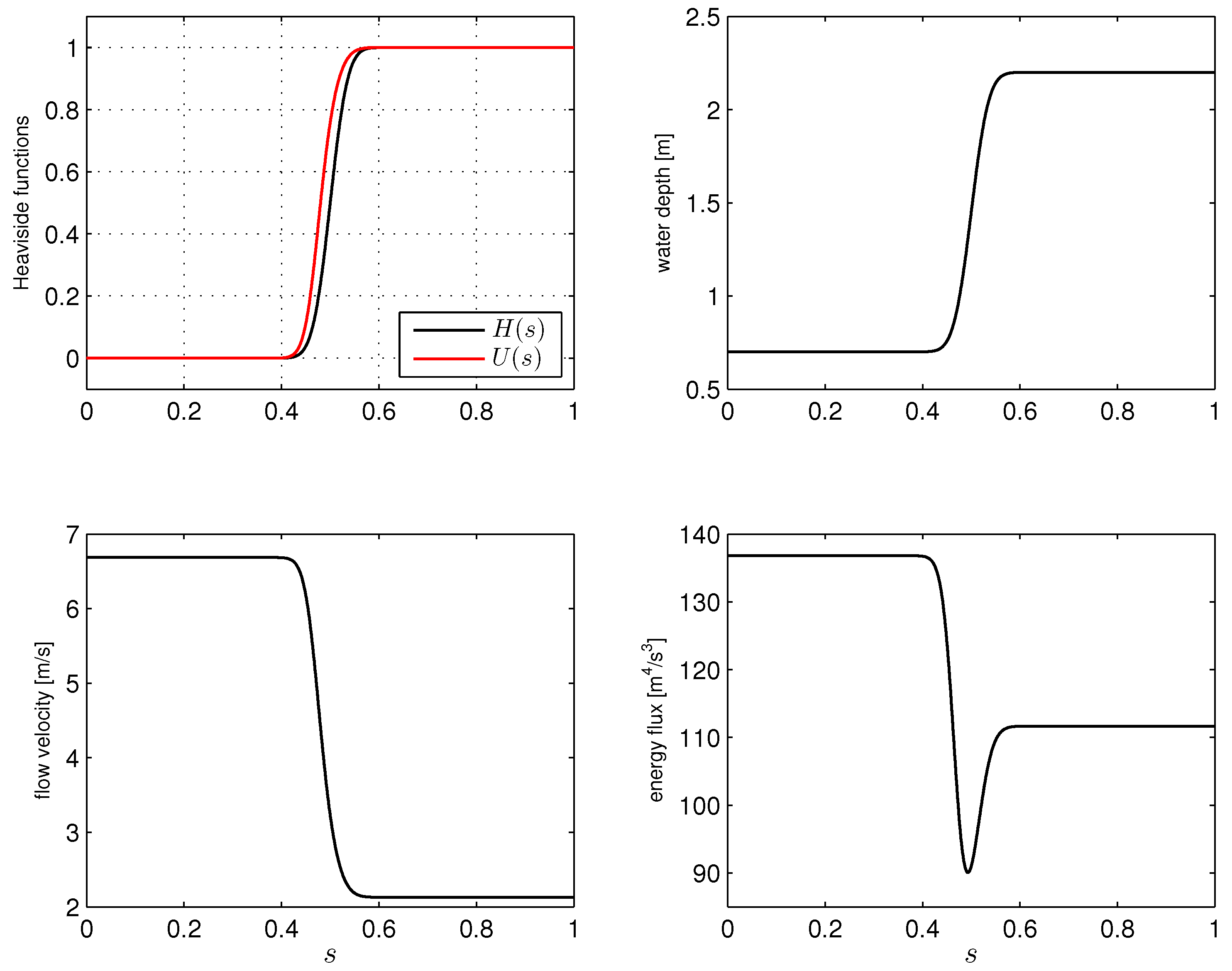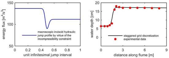To gain some insight on the solution regularization, Section 3 analyses the distribution of the flow field across the hydraulic jump, where the nonstandard Heaviside functions are employed to model smooth jump functions for the flow variables such as water depth, velocity and mechanical energy. A key result of this nonstandard analysis is that, unlike the primitive variables, the energy flux displays an undershoot in the hydraulic jump, suggesting that the viscosity does not play a crucial role, as similarly observed by Salas and Iollo [30], who demonstrated a local maximum of the entropy profile inside an inviscid gaseous shock. Numerical computations to study the formation of a hydraulic jump in a rectangular channel are performed as detailed in Section 4. Finally, conclusions are stated in Section 5.

2. Discretization of Shallow Water Equations from the Perspective of Nonstandard Calculus

2.1. Nonstandard Calculus

A complete introduction to nonstandard analysis can be found in the textbooks of Goldblatt [26] and Keisler [27]. In the following, the building blocks of nonstandard calculus, in particular, those used in this work, are briefly reviewed.

Basically, nonstandard analysis deals with an extension of the real number line $\mathbb{R}$ including nonzero infinitesimals and infinitely large numbers, along with the real numbers. This extended set is denoted by ${}^{*}\mathbb{R}$, and its elements are called hyperreals (or nonstandard reals). An infinitesimal is, in absolute value, a number that is smaller than every positive real number. Zero is the only real number that is an infinitesimal. The reciprocal of a nonzero infinitesimal is a hyperlarge number (or infinitely large or simply infinite), which is larger than any real number, though strictly smaller than infinity. If a number is not hyperlarge, it is called finite (or limited). Accordingly, every real number is finite. Finally, a number which is limited and not infinitesimal is called appreciable.

Neither nonzero infinitesimals nor infinitely large numbers exist on the real line. Yet, they can be treated in much the same way as standard numbers. This property is known as the transfer principle. As an example, the reals are an ordered field, and so are the hyperreals; infinitesimals differ in magnitude from other infinitesimals, and hyperlarge numbers from other hyperlarge numbers. For details on the construction of the nonstandard reals, we refer to Goldblatt [26].

Let $\epsilon$ be an infinitesimal and x and y be finite hyperreals. We define the relation $x\simeq y$ as $x-y$ is infinitesimal or zero. It immediately follows that $\epsilon \simeq 0$. This corollary essentially captures the idea of “arbitrary close” that lies at the heart of the well-known $\epsilon -\delta$ limit in calculus.

Furthermore, let a be a real number. The standard part of x, denoted by st(x), is a unique real a infinitely close to x, thus a = st(x). Consequently, $st\left(\epsilon \right)=0$. A hyperlarge number cannot have a standard part. The standard part function provides an essential link between the finite hyperreals and the real numbers.

Next to the hyperreal numbers, one also deals with hyperfunctions. Given a function f from $\mathbb{R}$ to $\mathbb{R}$, there is a unique function ${}^{*}f:{}^{*}\mathbb{R}\to {}^{*}\mathbb{R}$, called the *-transform of f, such that ${}^{*}f\left(x\right)=f\left(x\right)$ if and only if $x\in \mathbb{R}$. Thus, ${}^{*}f$ is a nonstandard extension of f.

Let $f:\mathbb{R}\to \mathbb{R}$, then the derivative of f at point x, denoted $f^{\prime }\left(x\right)$, is defined by

$$f^{\prime }\left(x\right)=st\left(\frac{{}^{*}f(x+\delta )-f\left(x\right)}{\delta }\right)$$

for every nonzero infinitesimal $\delta$, provided that $f^{\prime }\left(x\right)$ exists independent of $\delta$. Function f is said to be differentiable at point x. Notice that the derivative of f is not defined by a vanishing limit $\delta \to 0$, but as the standard part of a difference quotient; $f^{\prime }\left(x\right)$ is infinitesimally close to that quotient. As a basic example, we consider $f\left(x\right)=x^2$. Its derivative is calculated as follows:

$$f^{\prime }\left(x\right)=st\left(\frac{{(x+\delta )}^2-x^2}{\delta }\right)=st\left(2x+\delta \right)=st\left(2x\right)+st\left(\delta \right)=2x.$$

This example clearly demonstrates the effectiveness of using nonzero infinitesimals to determine the derivative without the need of an endless $\epsilon -\delta$ limiting process and, in turn, provides a rigorous basis for the calculus. For further illustrative examples, we refer to Keisler [27]. The transfer principle guarantees that all familiar rules involving derivatives, e.g., the product, quotient, and chain rules, also hold for hyperreal-valued functions.

Next, suppose that $f^{\prime }\left(x\right)$ exists at point x and let $\Delta x$ be a nonzero infinitesimal. Then, the increment of f, denoted $\Delta f$, due to change $\Delta x$ is given by

$$\Delta f={}^{*}f(x+\Delta x)-f\left(x\right)=f^{\prime }\left(x\right)\Delta x+\epsilon \Delta x$$

for some $\epsilon \simeq 0$. Consequently,

$$\frac{\Delta f}{\Delta x}=f^{\prime }\left(x\right)+\epsilon .$$

Thus, the standard part of the quotient $\Delta f/\Delta x$ equals the derivative $f^{\prime }\left(x\right)$. This result is known as the increment theorem. By virtue of the transfer principle, this property can be generalized to functions of multiple variables. Note that the infinitesimal $\epsilon$ can be viewed as an error term, which depends on $\Delta x$.

The use of infinitesimals in nonstandard analysis enables us to study topological spaces of reals induced by hyperfinite lattices. (Hyperfinite sets may be treated as finite sets, though they are generally infinite.) A halo (or a monad) of a point x on the hyperreal line is the interval of hyperreals that are infinitesimally close to x. Let $\mu \left(x\right)$ denote the halo of x, then $\mu \left(x\right)=\{y\in {}^{*}\mathbb{R}|y\simeq x\}$. While every point on the real line has zero dimensions, the size of each halo on the hyperreal line is infinitesimal. A halo is said to possess a microstructure. There exist infinitely large halos containing the point x. Furthermore, if x is finite, then $st\left(x\right)\in \mu \left(x\right)$, while not including other real numbers. Additionally, the halos of different real numbers do not overlap.

2.2. Discrete Formulations

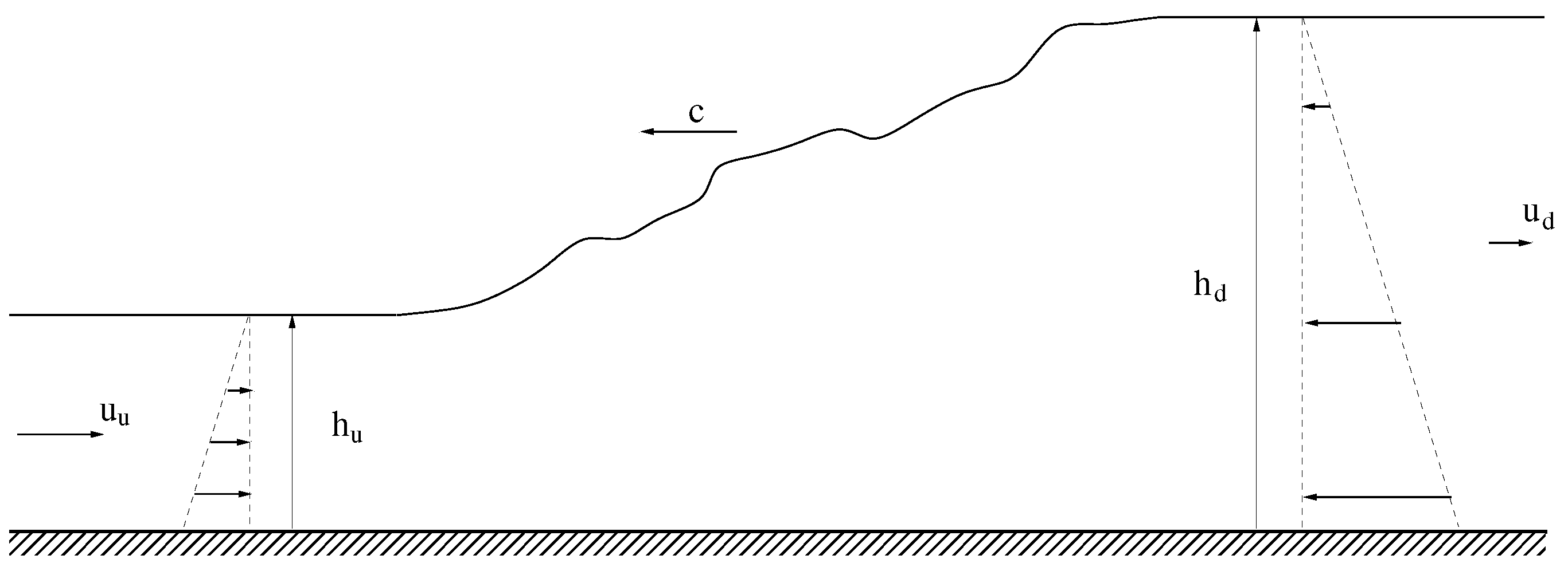
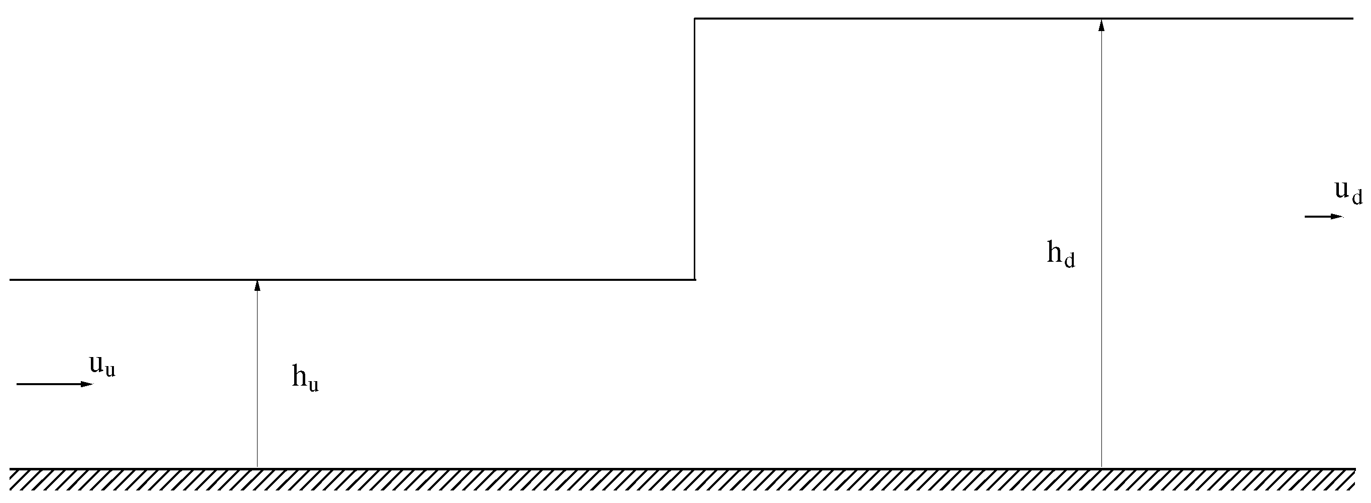
A hydraulic jump forms at the transition from the upstream supercritical flow to the downstream subcritical flow. A sudden rise subsequently occurs in the free surface while the flow is rapidly varied. Let us consider the hydraulic jump that moves at a constant speed c in an open channel with a uniform bed. The rate at which the flow changes between the upstream state and the downstream state is determined by the flow continuity and the momentum balance. Following Stoker [31], they can be written, respectively, in the following form

$$h_d\left(u_d-c\right)=h_u\left(u_u-c\right)$$

(1)

and

$$h_d\left(u_d-c\right)u_d-h_u\left(u_u-c\right)u_u=\frac{1}{2}g{h}_u^2-\frac{1}{2}g{h}_d^2.$$

(2)

Here, the variables h and u have their conventional meanings of water depth and flow velocity, whereas the subscripts u and d refer to the upstream and downstream states with respect to the jump; see Figure 1.

Furthermore, g is the acceleration of gravity. Note that the vertical pressure distribution away from the jump is hydrostatic.

Microscopically, due to viscous forces acting in the large flow gradients within the relatively thin jump layer, the flow is irreversible. Some of the kinetic energy is converted into an increase in potential energy and the remainder is lost through turbulence to heat. Consequently, the downstream state must have a higher entropy than the upstream state.

The rate of energy loss in flow expansion can be computed as follows (see [31]):

$$e_u-e_d=gq\frac{{\left(h_d-h_u\right)}^3}{4h_u{h}_d},$$

(3)

where $e_k=gq(h_k+{(u_k-c)}^2/2g)$ is the mechanical energy (flux) per unit mass (per unit width), with $k\in \{u,d\}$ labeling the position with respect to the jump, and $q=h_d(u_d-c)=h_u(u_u-c)$ is the mass flux through the jump.

The physical laws of mass conservation, momentum transport (Newton’s law of motion) and energy loss (the second law of thermodynamics) thus provide the macroscopic balance of flow changes across the hydraulic jump. In fact, this applies to any form of discontinuity that is intrinsically linked to an irreversible process. Yet, the resolution of Equations (1) and (2) adequately resolves the large-scale features of the flow field, while fluid motions that occur at length scales smaller than the width of the jump layer are not captured.

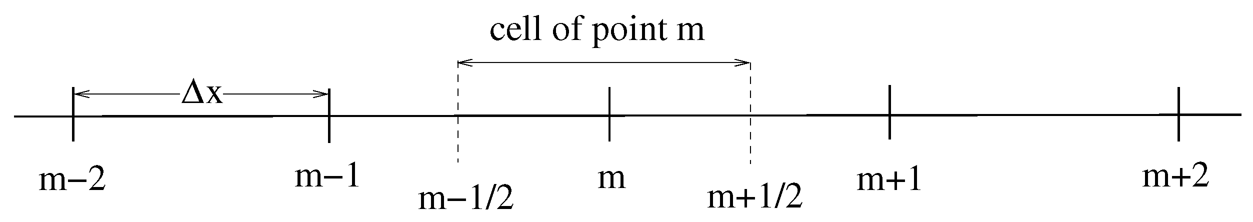
For the discussion below and in Section 3, and without loss of generality, we consider the channel with one dimension of space on the $x-$axis. The flow passes through the hydraulic jump in the positive $x-$direction. Accordingly, the traveling flow variables along a characteristic are a function of the similarity variable $s=x-ct$. By virtue of the increment theorem, we have

$$st\left(\frac{\Delta s}{\Delta x}\right)=\frac{\partial s}{\partial x}=1,st\left(\frac{\Delta s}{\Delta t}\right)=\frac{\partial s}{\partial t}=-c.$$

Let the jump be located at some point S on the characteristic. Now, the extension of the real number line to include nonzero infinitesimals naturally permits to deal with the set of all points separated from S by an infinitesimal distance. This halo of S, denoted $\mu \left(S\right)$, conceptually resolves the scale of the flow variables across the jump. The size of the halo is given by $\Delta s$, which is a nonzero infinitesimal.

Let the functions $h\left(s\right)$ and $u\left(s\right)$ be the water depth and flow velocity along the characteristic, respectively. These flow variables are constant on both sides of the infinitesimal jump. (Recall that the jump is uniformly moving with speed c.) Furthermore, the downstream state is distanced from the upstream one by $\Delta s$. Then, mass balance (1) with respect to the jump can be rewritten as

$$-c\left({}^{*}h(s+\frac{1}{2}\Delta s)-{}^{*}h(s-\frac{1}{2}\Delta s)\right)={}^{*}h(s-\frac{1}{2}\Delta s){}^{*}u(s-\frac{1}{2}\Delta s)-{}^{*}h(s+\frac{1}{2}\Delta s){}^{*}u(s+\frac{1}{2}\Delta s).$$

Using the variable transformation and a time shift of $+\frac{1}{2}\Delta t$, this equation is cast into

$$\begin{array}{ccc}& & \frac{{}^{*}h(x,t+\Delta t)\Delta x_a-h(x,t)\Delta x_a}{\Delta t}=\hfill \\ \hfill \\ & & {}^{*}h(x-\frac{1}{2}\Delta x,t+\frac{1}{2}\Delta t){}^{*}u(x-\frac{1}{2}\Delta x,t+\frac{1}{2}\Delta t)-{}^{*}h(x+\frac{1}{2}\Delta x,t+\frac{1}{2}\Delta t){}^{*}u(x+\frac{1}{2}\Delta x,t+\frac{1}{2}\Delta t)\hfill \end{array}$$

(4)

with $h(x,t)$ and $u(x,t)$ being the water depth and the flow velocity in the space-time domain, respectively. Note that point $(x,t)\in \mu \left(S\right)$ is finite. Furthermore, $\Delta t$ and $\Delta x$ are the nonzero infinitesimals associated with halo $\Delta s$. Finally, $\Delta x_a$ represents the infinitesimal area (per unit width) of the halo.

Physically, Equation (4) describes the volume balance with which the infinitesimal rate of change in the volume $h\Delta x_a$ of a halo is equated to the net mass flux $q=hu$ (inflow less outflow) through the boundaries of the halo. This naturally leads to the staggered positioning of the variables h and q in space and in time; the water depth is located at points intermediate between the mass fluxes. It should be noted that here the water depth (or the water level) undergoes a jump in the halo $\Delta x_a$.

The partial differential equation describing the conservation of volume can be inferred from the nonstandard Equation (4). Thus, noting that $\Delta x_a=\Delta x$, we have

$$\begin{array}{ccc}& & \frac{{}^{*}h(x,t+\Delta t)-h(x,t)}{\Delta t}+\hfill \\ \hfill \\ & & \frac{{}^{*}h(x+\frac{1}{2}\Delta x,t+\frac{1}{2}\Delta t){}^{*}u(x+\frac{1}{2}\Delta x,t+\frac{1}{2}\Delta t)-{}^{*}h(x-\frac{1}{2}\Delta x,t+\frac{1}{2}\Delta t){}^{*}u(x-\frac{1}{2}\Delta x,t+\frac{1}{2}\Delta t)}{\Delta x}=0\hfill \end{array}$$

and owing to the increment theorem, the standard part of this quotient yields

$$\frac{\partial h}{\partial t}+\frac{\partial hu}{\partial x}=0.$$

(5)

In the same way, we derive the momentum balance as follows. From Equation (2), we have

$$\begin{array}{ccc}& & -c\left({}^{*}h(s+\frac{1}{2}\Delta s){}^{*}u(s+\frac{1}{2}\Delta s)-{}^{*}h(s-\frac{1}{2}\Delta s){}^{*}u(s-\frac{1}{2}\Delta s)\right)+\hfill \\ \hfill \\ & & {}^{*}q(s+\frac{1}{2}\Delta s){}^{*}u(s+\frac{1}{2}\Delta s)-{}^{*}q(s-\frac{1}{2}\Delta s){}^{*}u(s-\frac{1}{2}\Delta s)=\frac{1}{2}g{}^{*}{h}^2(s-\frac{1}{2}\Delta s)-\frac{1}{2}g{}^{*}{h}^2(s+\frac{1}{2}\Delta s).\hfill \end{array}$$

This equation can be reshaped into space-time form as

$$\begin{array}{ccc}& & \frac{{}^{*}h(x+\frac{1}{2}\Delta x,t+\frac{1}{2}\Delta t){}^{*}u(x+\frac{1}{2}\Delta x,t+\frac{1}{2}\Delta t)\Delta x_l-{}^{*}h(x+\frac{1}{2}\Delta x,t-\frac{1}{2}\Delta t){}^{*}u(x+\frac{1}{2}\Delta x,t-\frac{1}{2}\Delta t)\Delta x_l}{\Delta t}\hfill \\ \hfill \\ & & +{}^{*}q(x+\Delta x,t){}^{*}u(x+\Delta x,t)-q(x,t)u(x,t)=\frac{1}{2}g{h}^2(x,t)-\frac{1}{2}g{}^{*}{h}^2(x+\Delta x,t)\hfill \end{array}$$

(6)

(note the space shift of $+\frac{1}{2}\Delta x$) or, with $\Delta x_l=\Delta x$, one obtains

$$\begin{array}{ccc}& & \frac{{}^{*}h(x+\frac{1}{2}\Delta x,t+\frac{1}{2}\Delta t){}^{*}u(x+\frac{1}{2}\Delta x,t+\frac{1}{2}\Delta t)-{}^{*}h(x+\frac{1}{2}\Delta x,t-\frac{1}{2}\Delta t){}^{*}u(x+\frac{1}{2}\Delta x,t-\frac{1}{2}\Delta t)}{\Delta t}+\hfill \\ \hfill \\ & & \frac{{}^{*}q(x+\Delta x,t){}^{*}u(x+\Delta x,t)-q(x,t)u(x,t)}{\Delta x}+\frac{\frac{1}{2}g{}^{*}{h}^2(x+\Delta x,t)-\frac{1}{2}g{h}^2(x,t)}{\Delta x}=0\hfill \end{array}$$

and its standard part is then given by

$$\frac{\partial hu}{\partial t}+\frac{\partial qu}{\partial x}+\frac{\partial \frac{1}{2}g{h}^2}{\partial x}=0.$$

(7)

Equation (6) describes the infinitesimal rate of change of the total momentum $hu\Delta x_l$ for an inviscid fluid within a halo $\Delta x_l$ through which the fluid flows. The first term on the left hand side is the local rate of change in momentum. Furthermore, the second and and the third term express the advective transfer of momentum with the mass flux q as the transporting velocity. This advective acceleration causes a nonlinear spatial change in the flow velocity u.

Now, the rate of change in momentum of the fluid is due to the action of hydrostatic pressure on the fluid on both sides of the halo as given by the right hand side of Equation (6). Again, the momentum and the pressure are carried at alternate spatial locations. Moreover, the direction of the flow acceleration is aligned with that of the net streamwise force. Accordingly, $\Delta x_l$ must be understood as the infinitesimal length of the path within the halo along which the momentum $hu$ (or depth-integrated velocity) is being transported. Thus, this momentum experiences a jump inside halo $\Delta x_l$.

A key feature of the discussed approach is the close association between the primary unknowns and the topology of the halo. In principle, the unknowns are the integrals over the points, lines, surfaces, and volumes, and are referred to as discrete forms of degree 0, 1, 2, and 3, respectively. Furthermore, they constitute a discrete representation for the primitive variables on a primal-dual pair of space lattices, which naturally induces staggering of the variables. For a more extensive survey of this topic, see Tonti [32] and Ferretti [29]. In the current depth-integrated framework, the area integral of h over $\Delta x_a$ (designated as the primal surface lattice of the halo) and the line integral of $hu$ along $\Delta x_l$ (i.e., the dual of the edge lattice of the halo $\Delta x_a$) are the discrete 2-form and 1-form, respectively.

2.3. Discussion

Equations (5) and (7) are the one-dimensional nonlinear shallow water equations with the unknowns h and $hu$, suitable for cases with horizontal frictionless beds. (A physically consistent extension to the case of flows over varying bottom topography with bed friction is dealt with in, e.g., [18,22]) Such continuous differential equations are routinely viewed as a mathematical model for describing the dynamics of a physical system while its number of degrees of freedom is infinity; their main merit resides precisely in their uniqueness and universality, that is, they uniquely describe physics at all scales.

The mathematical model for the inviscid shallow water equations is typically presented as a hyperbolic system of conservation laws (e.g., [8,11,16]). In one dimension, this system is of the form

$$\frac{\partial \mathbf{W}}{\partial t}+\frac{\partial \mathbf{F}}{\partial x}=\mathbf{S}(x,\mathbf{W}),\mathbf{W}(x,t)=\left(\begin{array}{c}h\\ hu\end{array}\right),\mathbf{F}\left(\mathbf{W}\right)=\left(\begin{array}{c}uh\\ u^{2}h+\frac{1}{2}g{h}^2\end{array}\right),$$

where $\mathbf{W}$ is the vector of conserved variables, $\mathbf{F}$ is the vector function of inviscid flux, and $\mathbf{S}$ is a source vector. Note that such vectors are expressed as field functions at a given point $(x,t)$ in the continuum. The mathematical structure of the hyperbolic system provides a good basis for the theory of weak solutions involving shock waves [3]. Nevertheless, this mathematical framework is general and does not take into account the physical nature of the variation of hydraulic jumps. In fact, the system may also admit non-physical discontinuous solutions.

Within the framework of (usually non-staggered) finite volume methods, a stable high-resolution scheme can be adopted with the aim of constructing the numerical flux vector. Then, the residual of the resulting algebraic equations (as computed by substituting the exact solution) acts as the principal source of discretization error. Provided that the solution is continuous and smooth, this error will be infinitesimally small.

However, the situation becomes different when the flow variables are discontinuous so that the solution error is no longer infinitesimal. If a hydraulic jump is located in $\mu \left(S\right)$, so that irreversible processes intervene, the solution of the difference equations is rather different from the solution of the differential equations. This divergence persists in the limit of vanishing size of $\mu \left(S\right)$. Obviously, the effect of discontinuity leaves no trace on the solution of differential equations. As explained above, this effect is basically discarded by an application of the standard part function, which in turn implies that the spatial features of the halo (here $\Delta x_a$ and $\Delta x_l$) are lost. This loss should be restored afterward by the discretization process. This generally calls for measures, often proposed heuristically, to ensure the entropy consistency of the discretization. Examples of such measures have been discussed in the introduction section of this paper.

By contrast, the nonstandard Equations (4) and (6) are principally considered to describe mathematically a physical system with a hyperlarge number of degrees of freedom [28]. This sole principle is built on the existence of nonzero infinitesimals. The resulting discrete equations establish the flow distribution within each infinitesimally small halo exhibiting a geometric structure, which may or may not contain a discontinuity. Furthermore, as it will be revealed in the next section, these equations have a built-in regularization effect on the solution.

The enrichment with a nonvanishing halo size is an essential feature because it paves the way towards grid partitioning of a flow domain. This feature provides a paradigm for constructing discretizations of the nonstandard equations that are naturally adapted for any type of grid system (Cartesian, curvilinear, and unstructured grids) and that behave correctly in a physical sense. By making the size of both $\Delta t$ and $\Delta x$ appreciable, the above system is translated into a finite but underdetermined system of equations. Its closure is commonly obtained by the addition of a number of constitutive (locally dependent) relations between the different solution fields, which involve the various interpolation (central and upwind) techniques. An example of this process of approximation can be found in Appendix A.

The development of mixed finite volume-finite difference methods that use C-grid staggering on two-dimensional structured and unstructured (triangular) meshes for the modeling of rapidly varied flows in coastal waters is documented in, e.g., [33,34,35,36,37].

3. Nonstandard Flow Profiles across Hydraulic Jump

3.1. Introduction

The aim of this section is to analyze one-dimensional jump distributions for an unsteady, incompressible, inviscid flow across an infinitesimal hydraulic jump on a horizontal bed by utilizing the nonstandard Heaviside functions. We adopt the methodology of Baty et al. [38], who advocate a rigorous approach based on nonstandard analysis to study the one-dimensional shock waves in a compressible, inviscid, perfect gas. However, to the best of our knowledge, no study has been reported for an inviscid hydrodynamic shock.

The significance of the present analysis is that it not only provides valuable insight into the jump solutions of water depth, flow velocity and mechanical energy, but also sheds light on the embedded regularization capability of the governing equations of motion. This is evident by the fact that the analysis deals with continuous hyperreal-valued functions mapped onto the set of hyperreal numbers instead of discontinuous real-valued functions that are mapped to real numbers. This is highly convenient, since it provides a rigorous justification for nonlinear problems that cannot be adequately addressed by the theory of distributions [39,40]. In particular, multiplications of differentiable nonstandard functions in the form of the Dirac delta function or the Heaviside step function are thus straightforward [38].

3.2. Nonstandard Heaviside Functions

The initial step of the analysis to be presented here is the introduction of nonstandard Heaviside step functions to properly represent the distribution of the flow field across the jump contained in a halo. Such functions belong to the class of infinitely differentiable functions.

A nonstandard Heaviside function is defined as follows:

$${}^{*}H\left(s\right)=\left\{\begin{array}{c}0,if\hspace{1em}s\le 0\hfill \\ \\ {}^{*}h\left(s\right),if\hspace{1em}0<s<\epsilon \hfill \\ \\ 1,if\hspace{1em}s\ge \epsilon \hfill \end{array}\right.$$

where $\epsilon$ is an infinitely small number, $s=x-ct$ is a characteristic with c a constant jump celerity, and ${}^{*}h\left(s\right)\in C^{\infty }(0,\epsilon )$ is a strictly increasing hyperreal-valued function representing an infinitesimal jump with thickness $\epsilon$ and

$${}^{*}h\left(0\right)=0,{}^{*}h\left(\epsilon \right)=1.$$

This function defines the microstructure (or the microscopic profile) of the flow field inside a shock layer [38,40]. The standard part of ${}^{*}H$ is unique and is given by

$$H\left(s\right)=st\left({}^{*}H\right)=\left\{\begin{array}{c}0,if\hspace{1em}s<0\hfill \\ 1,if\hspace{1em}s>0\hfill \end{array}\right..$$

In contrast to step function H, any function ${}^{*}H$ will support all of the operations in calculus required to derive solutions of the governing equations, in particular when dealing with nonlinear terms, e.g., the products of Heaviside functions. Indeed, by virtue of the definition of the standard Heaviside function, we have, for instance, $H^2\left(s\right)=H\left(s\right)$, but also $H^3\left(s\right)=H\left(s\right)$. Taking the derivative in both cases implies $2H{H}^{\prime }=H^{\prime }$ and $3H^2{H}^{\prime }=3H{H}^{\prime }=H^{\prime }$ with $H^{\prime }$ the Dirac delta function. Combining the last two equations yields $\frac{1}{2}{H}^{\prime }=\frac{1}{3}{H}^{\prime }$, which is false. By contrast, ${}^{*}{H}^k\left(s\right)\ne {}^{*}H\left(s\right)$ for all $k>1$, thus preventing this inconsistency.

Following Baty et al. [38] and Salas and Iollo [30], each flow variable is assumed to have a different microstructure. Thus, we look for solutions to h and u of the form

$$h\left(s\right)=h_u+\left[h\right]H\left(s\right),u\left(s\right)=u_u+\left[u\right]U\left(s\right),$$

(8)

where $\left[\varphi \right]\equiv {\varphi }_d-{\varphi }_u$ denotes the jump in variable $\varphi$. Recall that on both sides of the jump, the flow variables are constant. Since we are only dealing with nonstandard functions, we have omitted the superscript * for convenience. Furthermore, the Heaviside functions $H\left(s\right)$ and $U\left(s\right)$ are taken to have their jumps contained on the same interval $(0,\epsilon )$. In addition, they must satisfy the conditions at the endpoints of the halo, that is

$$H\left(0\right)=U\left(0\right)=0$$

and

$$H\left(\epsilon \right)=U\left(\epsilon \right)=1.$$

3.3. Jump Profiles for Flow Variables

To ease the process of deriving smooth functions of h and u from Equations (4) and (6), we adopt their standard parts expressed in nonconservative form. Note that the use of this form poses no problem for the present analysis since the Heaviside functions are differentiable [38]. (By contrast, the theories of weak solutions and distributions require the notion of conservation form.) Hence, we continue our analysis with the following nonlinear equations

$$\frac{\partial h}{\partial t}+u\frac{\partial h}{\partial x}+h\frac{\partial u}{\partial x}=0$$

(9)

and

$$\frac{\partial u}{\partial t}+u\frac{\partial u}{\partial x}+g\frac{\partial h}{\partial x}=0.$$

(10)

It is worth noting that the governing equations are strictly model equations based on two ideal, controlled conditions: the water is inviscid and incompressible. The latter implies no thermodynamic equation of state. Accordingly, the model equations do not contain enough physical information and consequently the microscopic flow profiles inside a shock layer cannot be deduced (see also [41]).

Another key issue is the local invalidity of the hydrostatic pressure assumption; the pressure cannot be hydrostatic inside the jump. This suggests that Equations (9) and (10) cannot be satisfied by the solutions as given in Equation (8). We verify this by direct substituting and subsequently arranging the resulting equations in matrix form. We then find

$$\left[\begin{array}{cc}(u-c)\left[h\right]& h\left[u\right]\\ g\left[h\right]& (u-c)\left[u\right]\end{array}\right]\left[\begin{array}{c}{H}^{\prime }\\ U^{\prime }\end{array}\right]=\left[\begin{array}{c}0\\ 0\end{array}\right],$$

where the prime denotes differentiation with respect to s. A non-trivial solution $[H^{\prime },U^{\prime }]$ exists if the matrix is singular. This is the case if

$$u-c=\sqrt{gh}$$

which corresponds to the critical flow condition that must be valid on the whole interval $(0,\epsilon )$. This would imply no jump. Thus, it is plausible to assert that Equation (10) does not describe the complete physics. Along with this finding, we will pursue the analysis by considering the continuity Equation (9) for which we will show below that regularization of the jump discontinuity is accomplished through this particular equation.

Since a distinct jump profile for each flow variable cannot be determined, we instead derive a relationship between the jump functions H and U. To this end, we substitute the jump solutions (8) into the continuity equation and subsequently rewrite the resulting equation by means of separation of H and U, as follows:

$$\frac{\left[u\right]U^{\prime }}{u_u-c+\left[u\right]U}=-\frac{\left[h\right]H^{\prime }}{h_u+\left[h\right]H}.$$

Integration gives

$$\alpha \left(u_u-c+\left[u\right]U\right)\left(h_u+\left[h\right]H\right)=1.$$

Upon making use of boundary conditions $H\left(0\right)=U\left(0\right)=0$, we obtain the integration constant

$$\alpha =\frac{1}{\left(u_u-c\right)h_u}$$

and, hence,

$$\left(u_u-c+\left[u\right]U\right)\left(h_u+\left[h\right]H\right)=\left(u_u-c\right)h_u.$$

(11)

We observe that the mass flux is constant inside the jump $(0,\epsilon )$ and is equal to q. Hence, no mass can be created nor destroyed within the hydrodynamic shock [42]. This is particularly important because it discloses the incompressibility constraint of the shallow water equations, which can be dealt with effectively by the use of staggered grids [22]. We further note that boundary conditions $H\left(\epsilon \right)=U\left(\epsilon \right)=1$ yield the Rankine–Hugoniot relation expressing the continuity of mass flux across the jump

$$\left(u_d-c\right)h_d=\left(u_u-c\right)h_u.$$

Finally, the sought relation follows from Equation (11)

$$U\left(s\right)=\frac{q}{\left[u\right]}\left[\frac{1}{h_u+\left[h\right]H\left(s\right)}-\frac{1}{h_u}\right].$$

(12)

This central result implies that the microstructure of the flow velocity differs from the microstructure of the water depth. Recall that these microstructures remain undetermined.

Note that besides the above jump condition of mass flux, another jump condition related to the conservation of momentum flux can be found. For this purpose, the momentum equation is written in the following form:

$$(u-c)h\left[u\right]U^{\prime }+gh\left[h\right]H^{\prime }=0$$

Recalling that $h=h_u+\left[h\right]H$ and the constant mass flux q, we obtain

$$g{\left[h\right]}^{2}H{H}^{\prime }+g{h}_u\left[h\right]H^{\prime }=-q\left[u\right]U^{\prime }$$

which is a nonlinear ordinary differential equation. Integrating both sides of this equation then yields

$$\frac{1}{2}g{\left[h\right]}^2{H}^2+g{h}_u\left[h\right]H=-q\left[u\right]U+\beta$$

with $\beta$ the constant of integration. With $H=U=0$ for $s=0$, the value of this constant is $\beta =0$. However, for $s=\epsilon$, we have $H=U=1$ and obtain the following Rankine–Hugoniot jump condition in the case of uniform bed (cf. Equation (2))

$$q\left[u\right]+\frac{1}{2}g\left[h^2\right]=0.$$

In view of the staggered grid discretization, the non-smooth transition across a hydraulic jump, as manifested by finite changes in the primitive variables u and h on either side of the jump in line with the above jump conditions, is effectively residing in one grid cell. The cellwise continuity of both mass and momentum flux is thus enforced by the staggered spatial placement of the unknowns and remains effective regardless of the grid size. By contrast, central finite volume schemes on non-staggered (or colocated) grids necessarily spread the discontinuity over two grid cells and also allow us to provoke the decoupling between odd and even grid cells. As a result, the constancy of mass and momentum fluxes across an abrupt change cannot be guaranteed. The importance of the Rankine–Hugoniot jump relations in the suppression of odd–even grid oscillations is elaborated in [22].

The remainder of the present section provides an analysis of a direct corollary of the above key result. In particular, we examine the jump distribution for mechanical energy per unit mass, which is given by

$$e\left(s\right)=gq\left(h\left(s\right)+\frac{{\left(u\left(s\right)-c\right)}^2}{2g}\right).$$

(13)

Like the other flow variables, function $e\left(s\right)$ is assumed to have its jump on the interval $(0,\epsilon )$. However, since it is a composite variable, we do not adopt the following solution form:

$$e\left(s\right)=e_u+\left[e\right]E\left(s\right),$$

where $E\left(s\right)$ is a nonstandard step function. Instead, we will show that function $e\left(s\right)$ exhibits a local extremum inside the hydraulic jump, considering that H is strictly increasing on $(0,\epsilon )$. Let the derivative $de/ds$ vanish at point ${\sigma }_p\in (0,\epsilon )$. Then,

$$0=\frac{de}{ds}=gq\left(\left[h\right]H^{\prime }\left({\sigma }_p\right)+\frac{u\left({\sigma }_p\right)-c}{g}\left[u\right]U^{\prime }\left({\sigma }_p\right)\right)$$

which implies

$$g\left[h\right]H^{\prime }\left({\sigma }_p\right)=-\left(u\left({\sigma }_p\right)-c\right)\left[u\right]U^{\prime }\left({\sigma }_p\right).$$

Recall Equation (12). Differentiation yields

$$U^{\prime }=-\frac{q}{\left[u\right]}\frac{\left[h\right]}{h^2}{H}^{\prime }.$$

Combining the last two equations and then using the fact that $H^{\prime }\left({\sigma }_p\right)>0$, we obtain

$${\left(u\left({\sigma }_p\right)-c\right)}^2=gh\left({\sigma }_p\right)$$

which is precisely the critical flow condition, corresponding to a Froude number of unity. Hence, the energy jump $e\left(s\right)$ is a non-decreasing function. Since energy is lost when the flow passes through the hydraulic jump, this function must take a minimum value at the critical flow.

As support for this finding, we consider the energy distribution across the jump at the microscopic scale. Within the shock layer, viscosity is then responsible for the redistribution and dissipation of mechanical energy. To show this, we first consider the following momentum equation including the viscous stress term

$$\frac{\partial hu}{\partial t}+\frac{\partial qu}{\partial x}+\frac{\partial \frac{1}{2}g{h}^2}{\partial x}=\frac{\partial }{\partial x}\left(\nu h\frac{\partial u}{\partial x}\right)$$

with $\nu$ the viscosity of water. Next, we derive the transport equation for the total energy (the sum of the kinetic energy and the potential energy but without bottom topography) by combining the momentum equation and continuity Equation (5). This equation reads

$$\frac{\partial \eta }{\partial t}+\frac{\partial G}{\partial x}=\frac{\partial }{\partial x}\left(\nu q\frac{\partial u}{\partial x}\right)-\nu h{\left(\frac{\partial u}{\partial x}\right)}^2,$$

(14)

where $\eta =\frac{1}{2}h{u}^2+\frac{1}{2}g{h}^2$ is the total energy (also termed entropy, see, e.g., [17]) and $G=q(\frac{1}{2}{u}^2+gh)$ is the entropy flux. The last term on the right hand side of Equation (14) results in a net loss of energy across the jump, while the first term redistributes the energy inside the hydraulic jump. In particular, the velocity upstream of the jump decreases rapidly, which in turn creates a sharp trough in the energy at the critical flow location, and then recovers towards the downstream side of the jump, which thus causes a rise in the energy level.

A similar phenomenon has been previously reported by Salas and Iollo [30], who have demonstrated the existence of an entropy overshoot inside an inviscid aerodynamic shock using the algebra of nonlinear generalized functions of Colombeau et al. [40]. Their finding has also been justified by the work of Baty and Margolin [41] using nonstandard analysis.

The conclusions that can be drawn from the present analysis are that despite being characterized by the complete absence of viscosity, the nonstandard Equations (4) and (6) do comply with the second law of thermodynamics, and the flow distribution inside the hydraulic jump is effectively regularized by the continuity equation. In particular, incompressibility is an essential component of the solution regularization.

The present analysis also offers support for the ability of the staggered grid approach to reproduce the macroscopic features of hydraulic jumps and bores such as the energy loss and the jump location. This will be further discussed in Section 4.

Yet, the numerical techniques for the solution of shallow water equations by which regularization is based on the addition of artificial dissipation, either explicitly (see, e.g., [14,16]) or implicitly (see, e.g., [8]), do not directly invoke the incompressibility constraint. Indeed, these methods are originally designed for the numerical solution of compressible Euler equations. (An in-depth study of the dissipative regularization of the compressible Euler (and Navier–Stokes) equations based on physical grounds is described in [43].)

3.4. An Illustrative Example

For the purpose of exploring the relation between the different microstructures of the flow field across an infinitesimal hydraulic jump, we introduce the nondimensional Heaviside function to model the microstructure for water depth h as defined by

$$H\left(s\right)=\frac{1}{2}+\frac{1}{2}erf\left[m\left(s-\frac{1}{2}\right)\right],$$

where s lies in the halo $\mathcal{I}=[0,1]$ (normalized by the jump thickness $\epsilon$) and $m\in {}^{*}\mathbb{N}$ is a fixed hyperinteger, either appreciable or infinitely large, that determines the actual thickness. It should be noted that the proposed error function is one way to represent a jump. Other examples of Heaviside functions to model the jump can be found in [41]. Also note that function H is monotone increasing on $\mathcal{I}$. The water depth profile is then given by

$$h\left(s\right)=h_u+\left(h_d-h_u\right)H\left(s\right).$$

The other variables are determined from this jump function, specifically flow velocity $u\left(s\right)$ and energy $e\left(s\right)$, by use of Equations (12) and (13), respectively. The nonstandard function $U\left(s\right)$ is likewise a monotone increasing function on $\mathcal{I}$.

We consider the case of a standing hydraulic jump ($c=0$) in a steady state, over a frictionless horizontal bed, as illustrated in Figure 2.

The corresponding flow is described by a depth $h_u$ and velocity $u_u$ upstream of the jump, and a depth $h_d$ and velocity $u_d$ downstream of the jump. The following values have been chosen for the present case: $h_u=0.7$ m, $u_u=6.7$ m/s, $h_d=2.2$ m and $u_d=2.1$ m/s. Note that these values satisfy Equations (1) and (2). Also note that $g=9.81$ m/s${}^2$. The upstream and downstream Froude numbers are found to be 2.55 and 0.46, respectively. The rate of energy loss in the jump is calculated from Equation (3)

$$e_u-e_d=25.2\frac{m^4}{s^3}.$$

(15)

The depth, velocity and energy jump profiles have been computed by setting $m=25$ and are presented in Figure 3.

It can be observed that the water depth and the flow velocity are monotonically increasing and decreasing, respectively, whereas the energy flux displays a sharp trough inside the jump. Furthermore, this undershoot does not affect the overall energy loss across the jump (cf. Equation (15)). The Froude number at the location of this undershoot ($s=0.5$) turns out to be exactly 1.

Overall, the present observations confirmed the results from the analysis of Section 3.3 and demonstrated that the undershoot observed in the energy profile inside the hydraulic jump is rooted in the continuity of mass flux across the shock because the microstructure associated with the water depth and the flow velocity is distinct, viz. Equation (12). Under the assumption of a strictly increasing function for the water depth in the microstructure $(0,\epsilon )$, this guarantees the existence of the entropy-consistent minimum value of energy in the shock.

4. Numerical Experiment

Gharangik and Chaudhry [14] reported both laboratory and numerical experiments to investigate the formation of a hydraulic jump in a rectangular flume with metal walls and bed. These include six test conditions with the upstream Froude number $F_u=u_u/\sqrt{g{h}_u}$ ranging from 2.3 to 7.0, and thus provide a useful benchmark solution for validating numerical methods. The objective of this test case is to assess the numerical efficiency of the staggered C-grid discretization as outlined in Section 2.2. Its complete description and implementation is given in Appendix A.

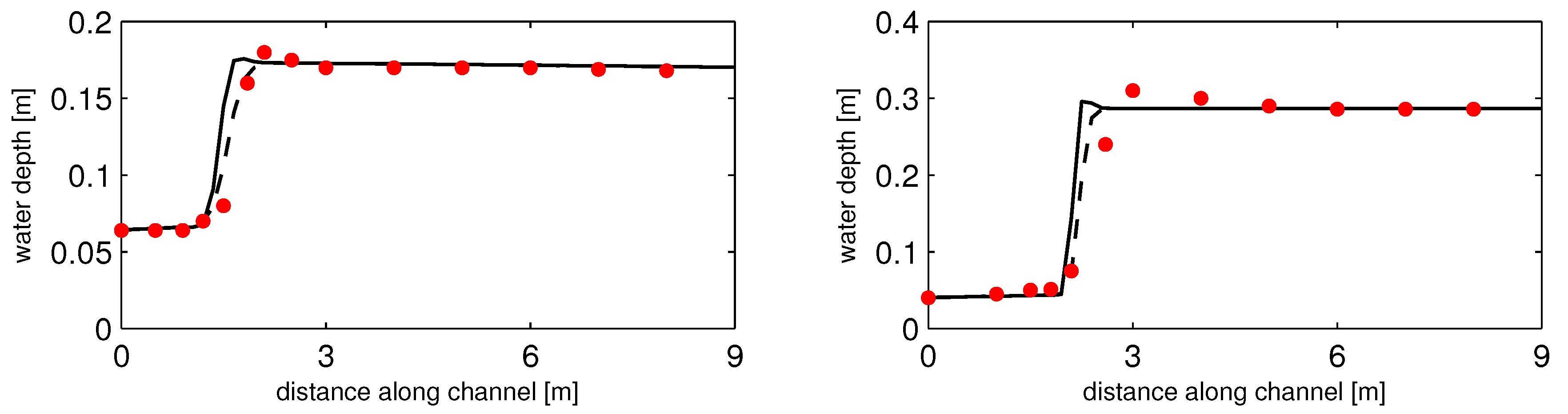
Numerical results of the current method are presented for two conditions: $F_u$ = 2.30 (test no. 6 of [14]) and $F_u$ = 5.74 (test no. 3). The flume dimensions and flow parameters for these cases are identical to those used by Gharangik and Chaudhry [14].

The computational grid was uniform and the grid size was set to 0.15 m. At the upstream boundary, an in-going Riemann invariant, defined as $u_u+2\sqrt{g{h}_u}$, was imposed, whereas at the downstream end the water depth $h_d$ was fixed. The time step was initially taken as 0.01 s and the Courant number was set equal to 0.5 (see Appendix A). The simulation time was set to 90 s, which was long enough to get a stabilized jump. Following Gharangik and Chaudhry [14], a Manning’s bed roughness coefficient of $k=0.008$ was adopted. No artificial viscosity nor flux limiting was applied in the course of simulations.

Numerical predictions and comparisons with the experimental data are depicted in Figure 4.

Here, the momentum advection is approximated by means of two upwind schemes: the first order upwind scheme (see Appendix A) and the second order Fromm’s scheme [44]. The latter scheme is designed for low numerical dispersion and dissipation.

Obviously, model-predicted jump profiles agree very well with the measurements. The location of the steady-state jump is adequately captured by the numerical approach. Additionally, the steepness of the jump profile is hardly affected by the amount of numerical diffusion induced by an advection scheme. This suggests that the role of this diffusion in the formation of the jump is less relevant than commonly believed. This finding is in line with the conclusion of Section 3.3.

To verify the correctness of the simulations the well-known Bélanger formula is employed and is given by

$$\frac{h_d}{h_u}=\frac{-1+\sqrt{1+8{F_u}^2}}{2}.$$

(16)

Based on the numerical outcomes, we observed a 5% lower ratio $h_d/h_u$ in comparison with Equation (16), which is acceptable.

It is further observed that there are virtually no spatial oscillations, albeit a small overshoot produced by the Fromm’s scheme. It should be noted that the numerical methods employed by Gharangik and Chaudhry [14] necessarily involve some amount of artificial viscosity to suppress these oscillations, and possibly numerical instability. The same conclusion is also found in [16]. The main cause of such oscillations is due to the non-staggered arrangement of the unknowns, which induces a checkerboard pattern. In turn, this can lead to a loss of continuity of the mass flux. Lastly, the study of Ginting [16] has also demonstrated the influence of the tuning of artificial viscosity on the jump location.

5. Conclusions

This paper provided an explanation of the ability of staggered C-grid discretizations to produce physically realistic results for rapidly varying free-surface flows by leveraging the concepts of nonstandard calculus. It was further argued that the physically consistent nonstandard equations governing the conservation of water volume and the streamwise transport of momentum can be established as a numerical methodology for solving the inviscid shallow water equations on staggered grids. The resulting discretization is characterized by the topological structures embedded in the nonstandard equations and the primary unknowns.

Nonstandard analysis also opens the door to adequately analyze nonlinear problems in the presence of discontinuities. The distributions of the water depth, flow velocity and mechanical energy across a one-dimensional infinitesimal thin inviscid hydraulic jump were analyzed by means of nonstandard Heaviside functions. The analysis presented in this work demonstrated that the modeled microstructure of the energy profile displays an undershoot inside the hydraulic jump, which is the result of the incompressibility constraint while the viscosity, either physical or artificial, plays no role. This principal result concludes that the staggered finite difference equations derived in this paper are effective for regularizing the entropy-consistent solution to the nonlinear shallow water equations.

The numerical results reported in this paper serve to illustrate that the numerical approach based on C-grid staggering indeed provides a superior representation of hydraulic jumps to that returned by the methods using artificial viscosity.

References

1. Lax, P.D. Weak solutions of nonlinear hyperbolic equations and their numerical computation. Comm. Pure Appl. Math. 1954, 7, 159–193. [Google Scholar] [CrossRef]
2. Lax, P.D.; Wendroff, B. Systems of conservation laws. Comm. Pure Appl. Math. 1960, 13, 217–237. [Google Scholar] [CrossRef] [Green Version]
3. LeVeque, R.J. Finite Volume Methods for Hyperbolic Problems; Cambridge University Press: Cambridge, UK, 2004. [Google Scholar]
4. Toro, E.F. Riemann Solvers and Numerical Methods for Fluid Dynamics: A Practical Introduction, 3rd ed.; Springer: Berlin, Germany, 2009. [Google Scholar]
5. Lax, P.D. Hyperbolic Systems of Conservation Laws and the Mathematical Theory of Shock Waves; SIAM: Philadelphia, PA, USA, 1973. [Google Scholar]
6. Harten, A.; Hyman, J.M. Self adjusting grid methods for one-dimensional hyperbolic conservation laws. J. Comput. Phys. 1983, 50, 235–269. [Google Scholar] [CrossRef]
7. Glaister, P. Approximate Riemann solutions of the shallow-water equations. J. Hydraul. Res. 1988, 26, 293–306. [Google Scholar] [CrossRef]
8. Alcrudo, F.; Garcia-Navarro, P. A high-resolution Godunov-type scheme in finite volumes for the 2D shallow-water equations. Int. J. Numer. Meth. Fluids 1993, 16, 489–505. [Google Scholar] [CrossRef]
9. Rogers, B.D.; Borthwick, A.G.L.; Taylor, P.H. Mathematical balancing of flux gradient and source terms prior to using Roe’s approximate Riemann solver. J. Comput. Phys. 2003, 192, 422–451. [Google Scholar] [CrossRef]
10. Audusse, E.; Bouchut, F.; Bristeau, M.O.; Klein, R.; Perthame, B. A fast and stable well-balanced scheme with hydrostatic reconstruction for shallow water flows. SIAM J. Sci. Comput. 2004, 25, 2050–2065. [Google Scholar] [CrossRef]
11. Kurganov, A.; Noelle, S.; Petrova, G. Semi-discrete central-upwind scheme for hyperbolic conservation laws and Hamilton-Jacobi equations. SIAM J. Sci. Comput. 2001, 23, 707–740. [Google Scholar] [CrossRef] [Green Version]
12. Kurganov, A.; Levy, D. Central-upwind schemes for the Saint-Venant system. M2AN Math. Model. Numer. Anal. 2002, 36, 397–425. [Google Scholar] [CrossRef] [Green Version]
13. Fennema, R.J.; Chaudhry, M.H. Explicit numerical schemes for unsteady free-surface flows with shocks. Water Resour. Res. 1986, 22, 1923–1930. [Google Scholar] [CrossRef]
14. Gharangik, A.M.; Chaudhry, M.H. Numerical simulation of hydraulic jump. J. Hydraul. Eng. 1991, 117, 1195–1211. [Google Scholar] [CrossRef]
15. Molls, T.R.; Zhao, G. Depth-averaged simulation of supercritical flow in channel with wavy sidewall. J. Hydraul. Eng. 2000, 126, 437–445. [Google Scholar] [CrossRef]
16. Ginting, B.M. A two-dimensional artificial viscosity technique for modelling discontinuity in shallow water flows. Appl. Math. Model. 2017, 45, 653–683. [Google Scholar] [CrossRef]
17. Fjordholm, U.S.; Mishra, S.; Tadmor, E. Well-balanced and energy stable schemes for the shallow water equations with discontinuous topography. J. Comput. Phys. 2011, 230, 5587–5609. [Google Scholar] [CrossRef] [Green Version]
18. Stelling, G.S.; Duinmeijer, S.P.A. A staggered conservative scheme for every Froude number in rapidly varied shallow water flows. Int. J. Numer. Meth. Fluids 2003, 43, 1329–1354. [Google Scholar] [CrossRef]
19. Kramer, S.C.; Stelling, G.S. A conservative unstructured scheme for rapidly varied flows. Int. J. Numer. Meth. Fluids 2008, 58, 183–212. [Google Scholar] [CrossRef]
20. Yamazaki, Y.; Kowalik, Z.; Cheung, K.F. Depth-integrated, non-hydrostatic model for wave breaking and run-up. Int. J. Numer. Meth. Fluids 2009, 61, 473–497. [Google Scholar] [CrossRef]
21. Doyen, D.; Gunawan, P.H. An explicit staggered finite volume scheme for the shallow water equations. In Finite Volumes for Complex Applications VII—Methods and Theoretical Aspects; Fuhrmann, J., Ohlberger, M., Rohde, C., Eds.; Springer: Cham, Switzerland, 2014; pp. 227–235. [Google Scholar]
22. Zijlema, M. The role of the Rankine-Hugoniot relations in staggered finite difference schemes for the shallow water equations. Comput. Fluids 2019, 192, 104274. [Google Scholar] [CrossRef]
23. Arakawa, A. Computational design for long-term numerical integration of the equations of fluid motion: Two-dimensional incompressible flow. Part I. J. Comput. Phys. 1966, 1, 119–143. [Google Scholar] [CrossRef]
24. Kleiner, I. History of the infinitely small and the infinitely large in calculus. Educ. Stud. Math. 2001, 48, 137–174. [Google Scholar] [CrossRef]
25. Lolli, G. Infinitesimals and infinites in the history of mathematics: A brief survey. Appl. Math. Comput. 2012, 218, 7979–7988. [Google Scholar] [CrossRef]
26. Goldblatt, R. Lectures on the Hyperreals: An Introduction to Nonstandard Analysis; Graduate Texts in Mathematics, 188; Springer: New York, NY, USA, 1998. [Google Scholar]
27. Keisler, H.J. Elementary Calculus: An Infinitesimal Approach, 2nd ed.; Dover: Kent, UK, 2002; Available online: http://www.math.wisc.edu/~keisler/calc.html (accessed on 16 May 2021).
28. Delfini, P.; Lobry, C. The vibrating string. In Nonstandard Analysis in Practice; Diener, F., Diener, M., Eds.; Springer: Berlin, Germany, 1995; Chapter 3; pp. 51–70. [Google Scholar]
29. Ferretti, E. The algebraic formulation: Why and how to use it. Curved Layer. Struct. 2015, 2, 106–149. [Google Scholar] [CrossRef]
30. Salas, M.D.; Iollo, A. Entropy jump across an inviscid shock wave. Theoret. Comput. Fluid Dyn. 1996, 8, 365–375. [Google Scholar] [CrossRef]
31. Stoker, J.J. Water Waves: The Mathematical Theory with Applications; Interscience Publishers: New York, NY, USA, 1957. [Google Scholar]
32. Tonti, E. Why starting from differential equations for computational physics? J. Comput. Phys. 2014, 257, 1260–1290. [Google Scholar] [CrossRef]
33. Yamazaki, Y.; Cheung, K.F.; Kowalik, Z. Depth-integrated, non-hydrostatic model with grid nesting for tsunami generation, propagation, and run up. Int. J. Numer. Meth. Fluids 2011, 67, 2081–2107. [Google Scholar] [CrossRef]
34. Zijlema, M.; Stelling, G.S.; Smit, P.B. SWASH: An operational public domain code for simulating wave fields and rapidly varied flows in coastal waters. Coast. Eng. 2011, 58, 992–1012. [Google Scholar] [CrossRef]
35. Kernkamp, H.W.J.; van Dam, A.; Stelling, G.S.; de Goede, E.D. Efficient scheme for the shallow water equations on unstructured grids with application to the Continental Shelf. Ocean Dyn. 2011, 61, 1175–1188. [Google Scholar] [CrossRef]
36. Kleptsova, O.; Pietrzak, J.D.; Stelling, G.S. On a momentum conservative z-layer unstructured C-grid ocean model with flooding. Ocean Modell. 2012, 54–55, 18–36. [Google Scholar] [CrossRef]
37. Zijlema, M. Computation of free surface waves in coastal waters with SWASH on unstructured grids. Comput. Fluids 2020, 213. [Google Scholar] [CrossRef]
38. Baty, R.S.; Farassat, F.; Tucker, D.H. Nonstandard analysis and shock wave jump conditions for converging shock waves. J. Math. Phys. 2008, 49, 063101. [Google Scholar] [CrossRef] [Green Version]
39. Colombeau, J.F.; Le Roux, A.Y. Multiplications of distributions in elasticity and hydrodynamics. J. Math. Phys. 1988, 29, 315–319. [Google Scholar] [CrossRef]
40. Colombeau, J.F.; Le Roux, A.Y.; Noussair, A.; Perrot, B. Microscopic profiles of shock waves and ambiguities in multiplications of distributions. SIAM J. Numer. Anal. 1989, 26, 871–883. [Google Scholar] [CrossRef]
41. Baty, R.S.; Margolin, L.G. Modern infinitesimals and the entropy jump across an inviscid shock wave. Int. J. Aeroacoust. 2018, 17, 502–520. [Google Scholar] [CrossRef]
42. Battjes, J.A.; Labeur, R.J. Unsteady Flow in Open Channels; Cambridge University Press: Cambridge, UK, 2017. [Google Scholar]
43. Margolin, L.G.; Baty, R.S. Conservation laws in discrete geometry. J. Geom. Mech. 2019, 11, 187–203. [Google Scholar] [CrossRef] [Green Version]
44. Fromm, J.E. A method for reducing dispersion in convective difference schemes. J. Comput. Phys. 1968, 3, 176–189. [Google Scholar] [CrossRef]
Figure 1. The hydraulic jump. The flow velocities are relative to the bed. The distribution of hydrostatic pressure is shown upstream and downstream of the jump. Definitions of the variables are provided in the text.
Mathematics 10 01387 g001
Figure 2. Schematic view of the hydraulic jump. The meaning of the variables is described in the text.
Mathematics 10 01387 g002
Figure 3. Heaviside functions and flow profiles across infinitesimal hydraulic jump with thickness of unity for m = 25 . Function H is based on the error function, while function U is computed with Equation (12).
Mathematics 10 01387 g003
Figure 4. Computed and recorded jump profiles for F u = 2.30 (left panel) and F u = 5.74 (right panel). Black solid line: present method using Fromm’s scheme; black dash line: present method using first order upwind scheme; red dots: experimental data of Gharangik and Chaudhry [14].
Mathematics 10 01387 g004
Publisher’s Note: MDPI stays neutral with regard to jurisdictional claims in published maps and institutional affiliations.