Zeroing Neural Network for Pseudoinversion of an Arbitrary Time-Varying Matrix Based on Singular Value Decomposition

Abstract

Many researchers have investigated the time-varying (TV) matrix pseudoinverse problem in recent years, for its importance in addressing TV problems in science and engineering. In this paper, the problem of calculating the inverse or pseudoinverse of an arbitrary TV real matrix is considered and addressed using the singular value decomposition (SVD) and the zeroing neural network (ZNN) approaches. Since SVD is frequently used to compute the inverse or pseudoinverse of a matrix, this research proposes a new ZNN model based on the SVD method as well as the technique of Tikhonov regularization, for solving the problem in continuous time. Numerical experiments, involving the pseudoinversion of square, rectangular, singular, and nonsingular input matrices, indicate that the proposed models are effective for solving the problem of the inversion or pseudoinversion of time varying matrices.

1. Introduction and Preliminaries

In this paper, the zeroing neural network (ZNN) approach is used to address the problem of calculating the inverse or pseudoinverse of an arbitrary time-varying (TV) real matrix. On the one hand, the pseudoinverse, or Moore–Penrose inverse, of $A\in {\mathbb{R}}^{m\times n}$ is the unique matrix $A^{†}$, such that the system of Penrose equations holds for $X:=A^{†}$ [1,2,3]:

$$A=AXA,X=XAX,{\left(XA\right)}^{\mathrm{T}}=XA,{\left(AX\right)}^{\mathrm{T}}=AX,$$

(1)

where $A^{\mathrm{T}}$ denotes the transpose of A. Note that, if A is a nonsingular square matrix, $A^{†}$ becomes the usual inverse $A^{-1}$. On the other hand, the singular value decomposition (SVD) of $A\in {\mathbb{R}}^{m\times n}$ is a factorization of the form [4]:

$$A=US{V}^{\mathrm{T}},$$

(2)

where $U\in {\mathbb{R}}^{m\times m}$ and $V\in {\mathbb{R}}^{n\times n}$ are orthogonal matrices, i.e., $U^{\mathrm{T}}=U^{-1}$ and $V^{\mathrm{T}}=V^{-1}$, while $S\in {\mathbb{R}}^{m\times n}$ is a rectangular (or square, in the case $m=n$) diagonal matrix with the singular values of A on its main diagonal. SVD is frequently used to compute the inverse or pseudoinverse of a matrix, while commonly existing in fields of scientific research, such as medical treatment and industrial applications, lattice computing [5], automatic classification of electromyograms [6], and face recognition [7]. In a recent work [8], the authors provided a zeroing neural network for computing the singular value decomposition of an arbitrary matrix. This work move things one step further, by designing a new ZNN model for calculating the inverse or pseudoinverse of an arbitrary TV matrix based on the singular value decomposition. For comparison purposes, we build another model based on direct pseudoinversion in accordance with the paper [9], and the experiments section demonstrates the efficacy of the proposed SVD model.

Zhang et al. in [10], developed a ZNN design for generating online solutions to TV problems. It is worth noting that most ZNN based dynamical systems fall under the category of recurrent neural networks (RNN) that are designed to find equation zeros. As a consequence, numerous valuable research findings have been presented in the literature. Addressing generalized inversion problems [11,12], tensor and matrix inversion problems [13], systems of linear equations [14,15], systems of matrix equations [14,16], quadratic optimization problems [17], and diverse matrix functions approximation [18,19] are the main applications of ZNNs. The first stage in developing ZNN dynamics is to design an error function $E\left(t\right)$ that is tailored to the underlying problem, commonly known as the Zhang function [20]. The second stage takes advantage of the proper dynamical evolution that follows:

$$\dot{E}\left(t\right)=\frac{\mathrm{d}E\left(t\right)}{\mathrm{d}t}=-\lambda \mathcal{F}\left(E\left(t\right)\right),$$

(3)

where $\dot{E}\left(t\right)\in {\mathbb{R}}^{m\times n}$ is the time derivative of $E\left(t\right)\in {\mathbb{R}}^{m\times n}$, $\lambda >0$ is the design parameter that is used for scaling the convergence, while $\mathcal{F}(·):{\mathbb{R}}^{m\times n}\to {\mathbb{R}}^{m\times n}$ means elementwise utilization of an odd and increasing activation function on $E\left(t\right)$. In our research, we will consider the ZNN evolution (3) under the linear activation function. That is,

$$\dot{E}\left(t\right)=\frac{\mathrm{d}E\left(t\right)}{\mathrm{d}t}=-\lambda E\left(t\right).$$

(4)

This work’s key points may be summarized as below:

• A novel ZNN approach, which is based on SVD, is employed for solving the problem of calculating the pseudoinverse of an arbitrary TV real matrix.
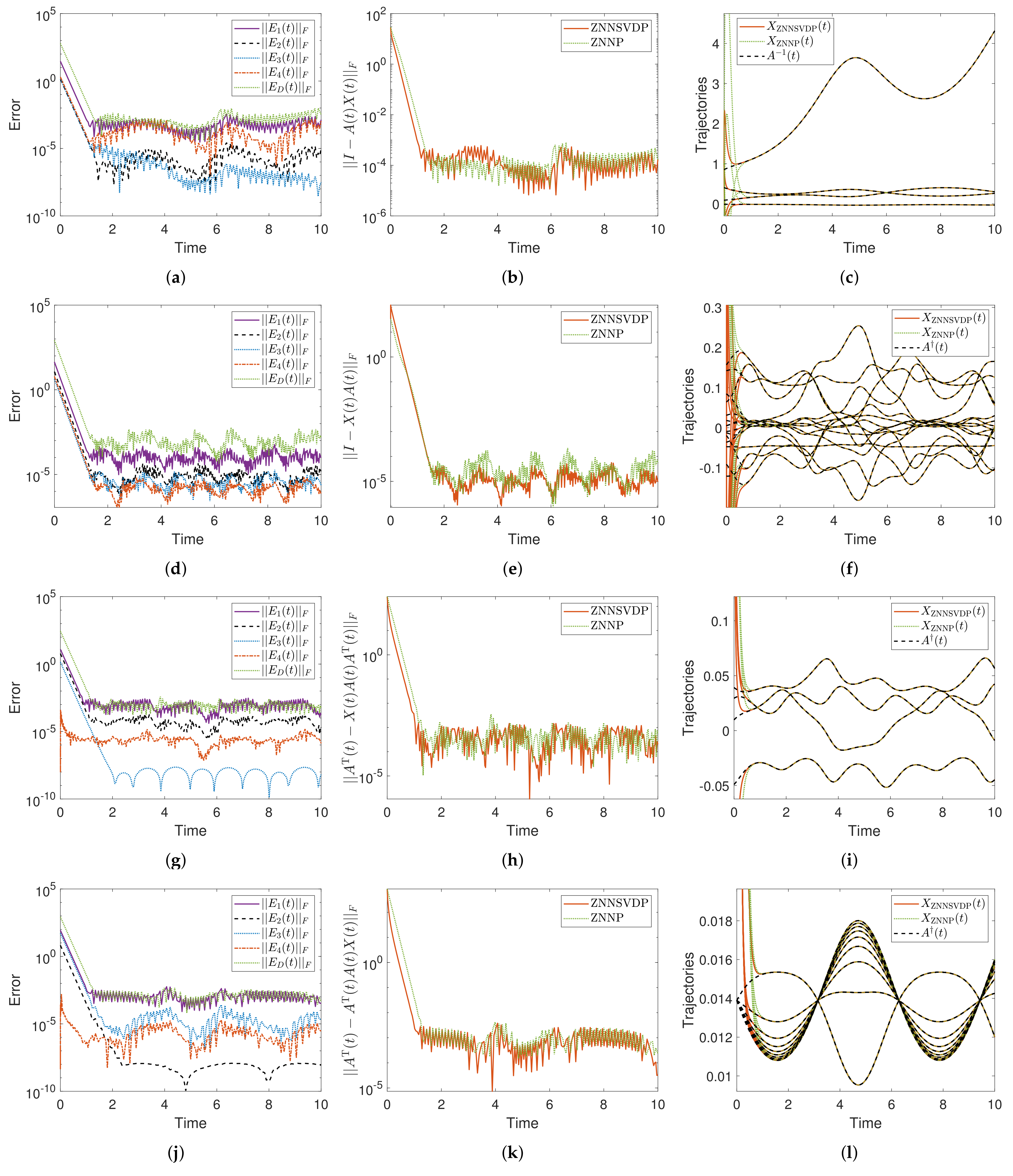
• Two ZNN models for calculating the pseudoinverse of an arbitrary TV matrix are offered: one called ZNNSVDP, which is based on SVD, and the other called ZNNP, which is based on a more direct approach to the problem and is offered for comparison purposes.
• Four numerical experiments, involving the pseudoinversion of square, rectangular, singular, and nonsingular input matrices, indicate that both models are effective for solving the problem and that the ZNNSVDP model converges to the problem’s solution faster than the ZNNP model.

Additionally, it is worth mentioning some of the paper’s general notations: the symbols ${\mathbf{1}}_n,{\mathbf{0}}_n$ denote a vector in ${\mathbb{R}}^n$ consisting of ones and zeros, respectively; ${\mathbf{O}}_{n\times n}\in {\mathbb{R}}^{n\times n}$ denotes a zero matrix of $n\times n$ dimensions; $I_n\in {\mathbb{R}}^{n\times n}$ denotes the identity $n\times n$ matrix; ⊗ denotes Kronecker product; $\mathrm{vec}(·)$ denotes the vectorization technique; ⊙ denotes the Hadamard (or element wise) product; and ${∥·∥}_F$ denotes the matrix Frobenius norm.

The paper is constituted as follows. Section 2 and Section 3, respectively, define and analyse the ZNNSVDP and ZNNP models. Section 4 presents and discusses the results of four numerical experiments employing the pseudoinversion of square, rectangular, singular, and nonsingular input matrices. Lastly, the final remarks and conclusions are offered in Section 5.

2. Time-Varying Pseudoinverse Computation Based on SVD

This section presents and analyses the ZNNSVDP model for calculating the pseudoinverse of an arbitrary TV real matrix. Considering a smooth TV matrix $A\left(t\right)\in {\mathbb{R}}^{m\times n}$, the inverse or pseudoinverse of $A\left(t\right)$ based on SVD (2) is the following:

$$\left\{\begin{array}{cc}{A}^{-1}\left(t\right)=V\left(t\right)S^{-1}\left(t\right)U^{\mathrm{T}}\left(t\right),\hfill & m=n=\mathrm{rank}\left(A\left(t\right)\right)\hfill \\ A^{†}\left(t\right)=V\left(t\right)S^{†}\left(t\right)U^{\mathrm{T}}\left(t\right),\hfill & \mathrm{otherwise},\hfill \end{array}\right.$$

(5)

where $U\left(t\right)\in {\mathbb{R}}^{m\times m}$ and $V\left(t\right)\in {\mathbb{R}}^{n\times n}$ are TV orthogonal matrices, and $S\left(t\right)\in {\mathbb{R}}^{m\times n}$ is a rectangular (or square, in the case $m=n$) diagonal matrix with the singular values of $A\left(t\right)$ on its main diagonal. Here, we consider decomposition so that the singular values of $A\left(t\right)$ are in descending order on the main diagonal of $S\left(t\right)$. Based on (2) and (5), the ZNNSVDP model considers the following group of error functions for calculating the inverse or pseudoinverse of $A\left(t\right)$:

$$\left\{\begin{array}{cc}{E}_1\left(t\right)=\hfill & A\left(t\right)V\left(t\right)-U\left(t\right)S\left(t\right)\hfill \\ E_2\left(t\right)=\hfill & U^{\mathrm{T}}\left(t\right)U\left(t\right)-I_m\hfill \\ E_3\left(t\right)=\hfill & V^{\mathrm{T}}\left(t\right)V\left(t\right)-I_n\hfill \\ E_4\left(t\right)=\hfill & X\left(t\right)-V\left(t\right)Y\left(t\right)U^{\mathrm{T}}\left(t\right),\hfill \end{array}\right.$$

(6)

where $X\left(t\right)$ is the desired solution of the problem, i.e., the inverse or pseudoinverse of $A\left(t\right)$, and

$$Y\left(t\right)=\left\{\begin{array}{cc}{S}^{-1}\left(t\right),\hfill & m=n=\mathrm{rank}\left(A\left(t\right)\right)\hfill \\ S^{†}\left(t\right),\hfill & \mathrm{otherwise}.\hfill \end{array}\right.$$

(7)

The following proposition about the structure and construction of the pseudoinverse of a diagonal matrix is offered, whereas [21] provides a full examination of this proposition.

Proposition 1.

For a rectangular (or a square singular) diagonal matrix $B\in {\mathbb{R}}^{m\times n}$, let $b_1,b_2\cdots ,b_w$ with $w=\mathrm{rank}\left(B\right)$ signify the elements of the main diagonal of B. Then, the pseudoinverse matrix of B is the following:

$$B^{†}=\left[\begin{array}{cc}{\overline{B}}^{-1}& {\mathbf{O}}_{w\times (n-w)}\\ {\mathbf{O}}_{(m-w)\times w}& {\mathbf{O}}_{(m-w)\times (n-w)}\end{array}\right],\mathrm{with}{\overline{B}}^{-1}=\left[\begin{array}{cccc}\frac{1}{b_1}& 0& \cdots & 0\\ 0& \frac{1}{b_2}& \cdots & 0\\ ⋮& ⋮& \ddots & ⋮\\ 0& 0& \cdots & \frac{1}{b_w}\end{array}\right].$$

(8)

In addition, the first time derivative of (6) is the following:

$$\left\{\begin{array}{cc}{\dot{E}}_1\left(t\right)=\hfill & \dot{A}\left(t\right)V\left(t\right)+A\left(t\right)\dot{V}\left(t\right)-\dot{U}\left(t\right)S\left(t\right)-U\left(t\right)\dot{S}\left(t\right)\hfill \\ {\dot{E}}_2\left(t\right)=\hfill & {\dot{U}}^{\mathrm{T}}\left(t\right)U\left(t\right)+U^{\mathrm{T}}\left(t\right)\dot{U}\left(t\right)\hfill \\ {\dot{E}}_3\left(t\right)=\hfill & {\dot{V}}^{\mathrm{T}}\left(t\right)V\left(t\right)+V^{\mathrm{T}}\left(t\right)\dot{V}\left(t\right)\hfill \\ {\dot{E}}_4\left(t\right)=\hfill & \dot{X}\left(t\right)-\dot{V}\left(t\right)Y\left(t\right)U^{\mathrm{T}}\left(t\right)-V\left(t\right)\dot{Y}\left(t\right)U^{\mathrm{T}}\left(t\right)-V\left(t\right)Y\left(t\right){\dot{U}}^{\mathrm{T}}\left(t\right),\hfill \end{array}\right.$$

(9)

where the first time derivative of $Y\left(t\right)$ is the following [22]:

$$\dot{Y}\left(t\right)=\left\{\begin{array}{cc}{\dot{S}}^{-1}\left(t\right)=\hfill & -S^{-1}\left(t\right)\dot{S}\left(t\right)S^{-1}\left(t\right),m=n=\mathrm{rank}\left(A\left(t\right)\right)\hfill \\ {\dot{S}}^{†}\left(t\right)=\hfill & -S^{†}\left(t\right)\dot{S}\left(t\right)S^{†}\left(t\right)+(S^{†}\left(t\right){(S^{†}\left(t\right))}^{\mathrm{T}}){\dot{S}}^{\mathrm{T}}\left(t\right)(I_m-S\left(t\right)S^{†}\left(t\right))\hfill \\ & +(I_n-S^{†}\left(t\right)S\left(t\right)){\dot{S}}^{\mathrm{T}}\left(t\right)({(S^{†}\left(t\right))}^{\mathrm{T}}{S}^{†}\left(t\right)),\mathrm{otherwise},\hfill \end{array}\right.$$

(10)

or equivalent

$$\begin{gathered} \dot{Y}\left(t\right)=-Y\left(t\right)\dot{S}\left(t\right)Y\left(t\right)+\left(Y\left(t\right)Y^{\mathrm{T}}\left(t\right)\right){\dot{S}}^{\mathrm{T}}\left(t\right)(I_m-S\left(t\right)Y\left(t\right)) \\ +(I_n-Y\left(t\right)S\left(t\right)){\dot{S}}^{\mathrm{T}}\left(t\right)\left(Y^{\mathrm{T}}\left(t\right)Y\left(t\right)\right). \end{gathered}$$

(11)

Notice that (11) is simplified to $\dot{Y}\left(t\right)=-Y\left(t\right)\dot{S}\left(t\right)Y\left(t\right)$ for $m=n=\mathrm{rank}\left(A\left(t\right)\right)$. Then, combining (6), (9) and (11) with the ZNN design under the linear activation function (4), the following may be acquired:

$$\left\{\begin{array}{cc}\dot{A}\left(t\right)V\hfill & \left(t\right)+A\left(t\right)\dot{V}\left(t\right)-\dot{U}\left(t\right)S\left(t\right)-U\left(t\right)\dot{S}\left(t\right)=-\lambda E_1(t)\hspace{1em}\hspace{1em}\hspace{1em}\hspace{1em}\hspace{1em}\hspace{1em}\hspace{1em}\hfill \\ {\dot{U}}^{\mathrm{T}}\left(t\right)\hfill & U\left(t\right)+U^{\mathrm{T}}\left(t\right)\dot{U}\left(t\right)=-\lambda E_2(t)\hspace{1em}\hspace{1em}\hspace{1em}\hspace{1em}\hspace{1em}\hspace{1em}\hspace{1em}\hfill \\ {\dot{V}}^{\mathrm{T}}\left(t\right)\hfill & V\left(t\right)+V^{\mathrm{T}}\left(t\right)\dot{V}\left(t\right)=-\lambda E_3(t)\hspace{1em}\hspace{1em}\hspace{1em}\hspace{1em}\hspace{1em}\hspace{1em}\hspace{1em}\hfill \\ \dot{X}\left(t\right)-\hfill & \dot{V}\left(t\right)Y\left(t\right)U^{\mathrm{T}}\left(t\right)-V\left(t\right)(-Y\left(t\right)\dot{S}\left(t\right)Y\left(t\right)+\left(Y\left(t\right)Y^{\mathrm{T}}\left(t\right)\right){\dot{S}}^{\mathrm{T}}\left(t\right)(I_m-S\left(t\right)Y\left(t\right))\hspace{1em}\hspace{1em}\hspace{1em}\hspace{1em}\hspace{1em}\hspace{1em}\hspace{1em}\hfill \\ & +(I_n-Y\left(t\right)S\left(t\right)){\dot{S}}^{\mathrm{T}}\left(t\right)\left(Y^{\mathrm{T}}\left(t\right)Y\left(t\right)\right))U^{\mathrm{T}}\left(t\right)-V\left(t\right)Y\left(t\right){\dot{U}}^{\mathrm{T}}\left(t\right)=-\lambda E_4\left(t\right).\hspace{1em}\hspace{1em}\hspace{1em}\hspace{1em}\hspace{1em}\hfill \end{array}\right.$$

(12)

Using vectorization and the Kronecker product, the dynamics of (12) are modified as follows:

$$\left\{\begin{array}{c}-(S^{\mathrm{T}}\left(t\right)\otimes I_m)\mathrm{vec}\left(\dot{U}\left(t\right)\right)+(I_n\otimes A\left(t\right))\mathrm{vec}\left(\dot{V}\left(t\right)\right)-(I_n\otimes U\left(t\right))\mathrm{vec}\left(\dot{S}\left(t\right)\right)\hfill \\ =\mathrm{vec}(-\lambda E_1\left(t\right)-\dot{A}\left(t\right)V\left(t\right))\hfill \\ (U^{\mathrm{T}}\left(t\right)\otimes I_m)\mathrm{vec}\left({\dot{U}}^{\mathrm{T}}\left(t\right)\right)+(I_m\otimes U^{\mathrm{T}}\left(t\right))\mathrm{vec}\left(\dot{U}\left(t\right)\right)=\mathrm{vec}(-\lambda E_2\left(t\right))\hfill \\ (V^{\mathrm{T}}\left(t\right)\otimes I_n)\mathrm{vec}\left({\dot{V}}^{\mathrm{T}}\left(t\right)\right)+(I_n\otimes V^{\mathrm{T}}\left(t\right))\mathrm{vec}\left(\dot{V}\left(t\right)\right)=\mathrm{vec}(-\lambda E_3\left(t\right))\hfill \\ -(I_m\otimes V\left(t\right)Y\left(t\right))\mathrm{vec}\left({\dot{U}}^{\mathrm{T}}\left(t\right)\right)-(U\left(t\right)Y^{\mathrm{T}}\left(t\right)\otimes I_n)\mathrm{vec}\left(\dot{V}\left(t\right)\right)-{\mathbf{K}}_1\left(t\right)+I_{mn}\mathrm{vec}\left(\dot{X}\left(t\right)\right)\hfill \\ =\mathrm{vec}(-\lambda E_4\left(t\right)),\hfill \end{array}\right.$$

(13)

where

$$\begin{gathered} {\mathbf{K}}_1\left(t\right)=-\left(U\left(t\right)Y^{\mathrm{T}}\left(t\right)\otimes V\left(t\right)Y\left(t\right)\right)\mathrm{vec}\left(\dot{S}\left(t\right)\right) \\ +\left(U\left(t\right){(I_m-S\left(t\right)Y\left(t\right))}^{\mathrm{T}}\otimes V\left(t\right)Y\left(t\right)Y^{\mathrm{T}}\left(t\right)\right)\mathrm{vec}\left({\dot{S}}^{\mathrm{T}}\left(t\right)\right) \\ +\left(U\left(t\right)Y^{\mathrm{T}}\left(t\right)Y\left(t\right)\otimes V\left(t\right)(I_n-Y\left(t\right)S\left(t\right))\right)\mathrm{vec}\left({\dot{S}}^{\mathrm{T}}\left(t\right)\right) \end{gathered}$$

(14)

Note that (13) must be simplified in order to produce a simple and explicit dynamical model that may easily calculate $U\left(t\right)$, $V\left(t\right)$, $S\left(t\right)$, and $X\left(t\right)$. As a result, the following lemmas about vectorization and the Kronecker product are offered, whereas [23] provides a full examination of Lemmas’ 1 and 2 content.

Lemma 1.

$$(L^{\mathrm{T}}\otimes A)\mathrm{vec}\left(X\right)=\mathrm{vec}\left(Y\right).$$

Lemma 2.

For $B\in {\mathbb{R}}^{m\times m}$, let $\mathrm{vec}\left(B\right)\in {\mathbb{R}}^{m^2}$ signify the matrix B vectorization. The following occurs:

$$\mathrm{vec}\left(B^{\mathrm{T}}\right)=Q_m\mathrm{vec}\left(B\right),$$

(15)

where $Q_m\in {\mathbb{R}}^{m^2\times m^2}$ is a constant permutation matrix defined exclusively by m.

The following, Algorithm 1, presents an algorithmic process for obtaining the permutation matrix $Q_m$ in (15), which corresponds to a matrix of $m\times m$ dimensions. Note that the notations eye(.) and reshape(.) in Algorithm 1 have the typical notion of the related MATLAB functions [24].

Algorithm 1 Permutation matrix calculation

Require: The rows or columns number m of a square matrix $B\in {\mathbb{R}}^{m\times m}$.

1: procedurePermutation_Matrix(m)

2:      Set $a=$ eye$\left(m^2\right)$ and $b=$ reshape$(1:m^2,m,m)$

3:      return $Q=a(:,$ reshape$(b^{\prime },1,m^2))$

4: end procedure

Ensure:$Q_m$, i.e., the permutation matrix.

Furthermore, because $S\left(t\right)$ and $S^{\mathrm{T}}\left(t\right)$ are rectangular (or square, in the case $m=n$) diagonal matrices, just the nonzero elements of $\dot{S}\left(t\right)$ and ${\dot{S}}^{\mathrm{T}}\left(t\right)$ that are placed in their main diagonal must be obtained. By doing so, we may confine $S\left(t\right)$ to being a diagonal matrix, while also reducing the dimensions of (13). Hence, employing the nonzero elements on the main diagonal of $S\left(t\right)$ and $S^{\mathrm{T}}\left(t\right)$, whose number is $w=\mathrm{rank}\left(A\left(t\right)\right)$, we utilize the equations $\mathrm{vec}\left(\dot{S}\left(t\right)\right)=G_1\dot{\mathbf{s}}\left(t\right)$ and $\mathrm{vec}\left({\dot{S}}^{\mathrm{T}}\left(t\right)\right)=G_2\dot{\mathbf{s}}\left(t\right)$, respectively, to replace $\dot{S}\left(t\right)$ and ${\dot{S}}^{\mathrm{T}}\left(t\right)$ in (14), where the matrices $G_1,G_2\in {\mathbb{R}}^{mn\times w}$ are operational matrices that can be calculated using the algorithmic procedure presented Algorithm 2. Additionally, the notation sum(.), min(.), zeros(.), mod(.) and floor(.) in Algorithm 2 have the typical notion of the related MATLAB functions [24].

Algorithm 2 Operational matrix calculation

Require: The number of the rows and columns, respectively, m and n of a matrix $B\in {\mathbb{R}}^{m\times n}$,

and $w=\mathrm{rank}\left(B\right)$.

1:  procedureOperational_Matrix($m,n,w$)

2:     if $w<min(m,n)$ then

3:        Set $h=w$

4:    else

5:        Set $h=m$

6:    end if

7:    Set $G=$ zeros$(mn,w)$

8:    for $k=1:mn$ do

9:        Set $c=$ mod$(k-1,h)+1$ and $d=$ floor$\left(\frac{k-1}{h}\right)+1$

10:        if $d==c$ then

11:           Set $G(k,c)=1$

12:        end if

13:    end for

14:    return G

15: end procedure

Ensure: The operational matrix G.

Based on the aforementioned discussion, (13) can be reformulated as follows:

$$\left\{\begin{array}{c}-(S^{\mathrm{T}}\left(t\right)\otimes I_m)\mathrm{vec}\left(\dot{U}\left(t\right)\right)+(I_n\otimes A\left(t\right))\mathrm{vec}\left(\dot{V}\left(t\right)\right)-(I_n\otimes U\left(t\right))G_1\dot{\mathbf{s}}\left(t\right)\hfill \\ =\mathrm{vec}(-\lambda E_1\left(t\right)-\dot{A}\left(t\right)V\left(t\right))\hfill \\ (U^{\mathrm{T}}\left(t\right)\otimes I_m)Q_m\mathrm{vec}\left(\dot{U}\left(t\right)\right)+(I_m\otimes U^{\mathrm{T}}\left(t\right))\mathrm{vec}\left(\dot{U}\left(t\right)\right)=\mathrm{vec}(-\lambda E_2\left(t\right))\hfill \\ (V^{\mathrm{T}}\left(t\right)\otimes I_n)Q_n\mathrm{vec}\left(\dot{V}\left(t\right)\right)+(I_n\otimes V^{\mathrm{T}}\left(t\right))\mathrm{vec}\left(\dot{V}\left(t\right)\right)=\mathrm{vec}(-\lambda E_3\left(t\right))\hfill \\ -(I_m\otimes V\left(t\right)Y\left(t\right))\mathrm{vec}\left({\dot{U}}^{\mathrm{T}}\left(t\right)\right)-(U\left(t\right)Y^{\mathrm{T}}\left(t\right)\otimes I_n)\mathrm{vec}\left(\dot{V}\left(t\right)\right)-{\mathbf{K}}_2\left(t\right)\dot{\mathbf{s}}\left(t\right)\hfill \\ +I_{mn}\mathrm{vec}\left(\dot{X}\left(t\right)\right)=\mathrm{vec}(-\lambda E_4\left(t\right)),\hfill \end{array}\right.$$

(16)

where

$$\begin{gathered} {\mathbf{K}}_2\left(t\right)=-\left(U\left(t\right)Y^{\mathrm{T}}\left(t\right)\otimes V\left(t\right)Y\left(t\right)\right)G_1 \\ +\left(U\left(t\right){(I_m-S\left(t\right)Y\left(t\right))}^{\mathrm{T}}\otimes V\left(t\right)Y\left(t\right)Y^{\mathrm{T}}\left(t\right)\right)G_2 \\ +\left(U\left(t\right)Y^{\mathrm{T}}\left(t\right)Y\left(t\right)\otimes V\left(t\right)(I_n-Y\left(t\right)S\left(t\right))\right)G_2 \end{gathered}$$

(17)

As a result, setting

$$\begin{gathered} Z_1\left(t\right)=\left[\begin{array}{c}-(S^{\mathrm{T}}\left(t\right)\otimes I_m)\\ (U^{\mathrm{T}}\left(t\right)\otimes I_m)Q_m+(I_m\otimes U^{\mathrm{T}}\left(t\right))\\ {\mathbf{0}}_{n^2\times m^2}\\ -(I_m\otimes V\left(t\right)Y\left(t\right))\end{array}\right],Z_3\left(t\right)=\left[\begin{array}{c}-(I_n\otimes U\left(t\right))G_1\\ {\mathbf{0}}_{m^2\times w}\\ {\mathbf{0}}_{n^2\times w}\\ -{\mathbf{K}}_2\left(t\right)\end{array}\right], \\ {Z}_2\left(t\right)=\left[\begin{array}{c}(I_n\otimes A\left(t\right))\\ {\mathbf{0}}_{m^2\times n^2}\\ (V^{\mathrm{T}}\left(t\right)\otimes I_n)Q_n+(I_n\otimes V^{\mathrm{T}}\left(t\right))\\ -(U\left(t\right)Y^{\mathrm{T}}\left(t\right)\otimes I_n)\end{array}\right],Z_4\left(t\right)=\left[\begin{array}{c}{\mathbf{0}}_{mn\times mn}\\ {\mathbf{0}}_{m^2\times mn}\\ {\mathbf{0}}_{n^2\times mn}\\ I_{mn}\end{array}\right],\hspace{1em}\hspace{1em}\hspace{1em}\hspace{1em} \\ Z\left(t\right)=\left[\begin{array}{cccc}{Z}_1\left(t\right)& Z_2\left(t\right)& Z_3\left(t\right)& Z_4\left(t\right)\end{array}\right],\hspace{1em}\hspace{1em}\hspace{1em}\hspace{1em}\hspace{1em}\hspace{1em}\hspace{1em}\hspace{1em}\hspace{1em}\hspace{1em}\hspace{1em}\hspace{1em}\hspace{1em}\hspace{1em}\hspace{1em}\hspace{1em}\hspace{1em}\hspace{1em} \end{gathered}$$

(18)

$$q\left(t\right)={\left[\begin{array}{c}\mathrm{vec}(-\lambda E_1\left(t\right)-\dot{A}\left(t\right)V\left(t\right))\\ \mathrm{vec}(-\lambda E_2\left(t\right))\\ \mathrm{vec}(-\lambda E_3\left(t\right))\\ \mathrm{vec}(-\lambda E_4\left(t\right))\end{array}\right]}^{\mathrm{T}},\dot{\mathbf{x}}=\left[\begin{array}{c}\mathrm{vec}\left(\dot{U}\left(t\right)\right)\\ \mathrm{vec}\left(\dot{V}\left(t\right)\right)\\ \mathrm{vec}\left(\dot{\mathbf{s}}\left(t\right)\right)\\ \mathrm{vec}\left(\dot{X}\left(t\right)\right)\end{array}\right],\mathbf{x}=\left[\begin{array}{c}\mathrm{vec}\left(U\right(t\left)\right)\\ \mathrm{vec}\left(V\right(t\left)\right)\\ \mathrm{vec}\left(\mathbf{s}\right(t\left)\right)\\ \mathrm{vec}\left(X\right(t\left)\right)\end{array}\right],$$

(19)

we propose the following ZNN model:

$$Z^{\mathrm{T}}\left(t\right)Z\left(t\right)\dot{\mathbf{x}}\left(t\right)=Z^{\mathrm{T}}\left(t\right)q\left(t\right),$$

(20)

where $Z^{\mathrm{T}}\left(t\right)Z\left(t\right)$ is a singular mass matrix. To solve the singularity problem, the Tikhonov regularization is used and (20) is converted into:

$$(Z^{\mathrm{T}}\left(t\right)Z\left(t\right)+\beta I_{m^2+n^2+w+mn})\dot{\mathbf{x}}\left(t\right)=Z^{\mathrm{T}}\left(t\right)q\left(t\right),$$

(21)

where $\beta \ge 0$ signifies the regularization parameter. The ZNN model (21) is termed as the ZNNSVDP model and can be solved efficiently with an appropriate ode Matlab solver. The exponential convergence of the ZNNSVDP model (21) to the theoretical TV inverse or pseudoinverse of the input matrix $A\left(t\right)$ is proven in Theorem 1.

Remark 1.

According to MATLAB’sodesolvers syntax [24], the mass matrix is a symmetric matrix M that expresses the connection between the time derivative $\dot{x}$ of the generalized coordinate vector x of a system, by the equation:

$$M\dot{x}=x.$$

Theorem 1.

Let $U\left(t\right)\in {\mathbb{R}}^{m\times m},V\left(t\right),\in {\mathbb{R}}^{n\times n},S\left(t\right)\in {\mathbb{R}}^{m\times n}$ be differentiable and $S\left(t\right)$ be a rectangular diagonal matrix. The ZNNSVDP model (21), starting from any initial value $\mathbf{x}\left(0\right)$, converges exponentially to the theoretical TV inverse or pseudoinverse of the input matrix $A\left(t\right)$.

Proof. 

In order to obtain the solution $\mathbf{x}\left(t\right)$, which corresponds to the TV inverse or pseudoinverse of the input matrix $A\left(t\right)$, the error matrix equation group is defined as in (9), inline with the ZNN design. Following that, by adopting the linear design formula for zeroing (9), the model (12) is obtained. From [Theorem 1] [10], each error matrix equation in the error matrix equation group (12) converges exponentially to the theoretical solution when $t\to \infty$. As a result, the solution of (12) converges exponentially to the theoretical TV inverse or pseudoinverse of the input matrix $A\left(t\right)$ when $t\to \infty$. Furthermore, from the derivation procedure of (21) from (12), the proof is completed.    □

3. Alternative Time-Varying Pseudoinverse Computation

This section presents and analyzes a ZNN model, namely, ZNNP, for calculating the pseudoinverse of any TV real matrix, based on a recent work [9] on ZNN pseudoinverse computation, and this new model will serve as a strong and fair competitor to the proposed ZNNSVDP model. Considering a smooth TV matrix $A\left(t\right)\in {\mathbb{R}}^{m\times n}$, then, if $\mathrm{rank}\left(A\right(t\left)\right)=n<m$, the MP inverse $A^{†}\left(t\right)$ becomes the left inverse $A^{†}\left(t\right)=A_L^{-1}\left(t\right)\equiv {\left(A^{\mathrm{T}}\left(t\right)A\left(t\right)\right)}^{-1}{A}^{\mathrm{T}}\left(t\right)$ of $A\left(t\right)$, where $A^{\mathrm{T}}\left(t\right)A\left(t\right)A^{†}\left(t\right)=A^{\mathrm{T}}\left(t\right)$. Otherwise, if $\mathrm{rank}\left(A\right(t\left)\right)=n>m$, the MP inverse $A^{†}\left(t\right)$ becomes the right inverse $A^{†}\left(t\right)=A_R^{-1}\left(t\right)\equiv A^{\mathrm{T}}\left(t\right){\left(A\left(t\right)A^{\mathrm{T}}\left(t\right)\right)}^{-1}$, where $A^{†}\left(t\right)A\left(t\right)A^{\mathrm{T}}\left(t\right)=A^{\mathrm{T}}\left(t\right)$. Therefore, we can design a ZNN model according to the following equations:

$$\left\{\begin{array}{cc}{A}^{\mathrm{T}}\left(t\right)A\left(t\right)A^{-1}\left(t\right)=A^{\mathrm{T}}\left(t\right),\hfill & m=n=\mathrm{rank}\left(A\left(t\right)\right)\hfill \\ A^{\mathrm{T}}\left(t\right)A\left(t\right)A^{†}\left(t\right)=A^{\mathrm{T}}\left(t\right),\hfill & \mathrm{rank}\left(A\left(t\right)\right)\le n<m\hfill \\ A^{†}\left(t\right)A\left(t\right)A^{\mathrm{T}}\left(t\right)=A^{\mathrm{T}}\left(t\right),\hfill & \mathrm{rank}\left(A\left(t\right)\right)\le m<n.\hfill \end{array}\right.$$

(22)

Based on (22), the ZNNP model considers the following error function for calculating the inverse or pseudoinverse of $A\left(t\right)$:

$$E_D\left(t\right)=\left\{\begin{array}{cc}{A}^{\mathrm{T}}\left(t\right)A\left(t\right)X\left(t\right)-A^{\mathrm{T}}\left(t\right),\hfill & \mathrm{rank}\left(A\left(t\right)\right)\le n\le m\hfill \\ X\left(t\right)A\left(t\right)A^{\mathrm{T}}\left(t\right)-A^{\mathrm{T}}\left(t\right),\hfill & \mathrm{rank}\left(A\left(t\right)\right)\le m<n.\hfill \end{array}\right.$$

(23)

where $X\left(t\right)$ is the desired solution of the problem, i.e., the inverse or pseudoinverse of $A\left(t\right)$. Furthermore, the first time derivative of (23) is the following:

$${\dot{E}}_D\left(t\right)=\left\{\begin{array}{cc}{\dot{A}}^{\mathrm{T}}\left(t\right)A\left(t\right)X\left(t\right)+A^{\mathrm{T}}\left(t\right)\dot{A}\left(t\right)X\left(t\right)+A^{\mathrm{T}}\left(t\right)A\left(t\right)\dot{X}\left(t\right)-{\dot{A}}^{\mathrm{T}}\left(t\right),\hfill & \mathrm{rank}\left(A\left(t\right)\right)\le n\le m\hfill \\ \dot{X}\left(t\right)A\left(t\right)A^{\mathrm{T}}\left(t\right)+X\left(t\right)\dot{A}\left(t\right)A^{\mathrm{T}}\left(t\right)+X\left(t\right)A\left(t\right){\dot{A}}^{\mathrm{T}}\left(t\right)-{\dot{A}}^{\mathrm{T}}\left(t\right),\hfill & \mathrm{rank}\left(A\left(t\right)\right)\le m<n.\hfill \end{array}\right.$$

(24)

Then, combining (23) and (24) with the ZNN design (4), under the linear activation function, the following can be obtained:

$$\left\{\begin{array}{cc}{\dot{A}}^{\mathrm{T}}\left(t\right)A\left(t\right)X\left(t\right)\hfill & +A^{\mathrm{T}}\left(t\right)\dot{A}\left(t\right)X\left(t\right)+A^{\mathrm{T}}\left(t\right)A\left(t\right)\dot{X}\left(t\right)-{\dot{A}}^{\mathrm{T}}\left(t\right)\hfill \\ & =-\lambda (A^{\mathrm{T}}\left(t\right)A\left(t\right)X\left(t\right)-A^{\mathrm{T}}\left(t\right)),\mathrm{rank}\left(A\left(t\right)\right)\le n\le m\hfill \\ \dot{X}\left(t\right)A\left(t\right)A^{\mathrm{T}}\left(t\right)\hfill & +X\left(t\right)\dot{A}\left(t\right)A^{\mathrm{T}}\left(t\right)+X\left(t\right)A\left(t\right){\dot{A}}^{\mathrm{T}}\left(t\right)-{\dot{A}}^{\mathrm{T}}\left(t\right)\hfill \\ & =-\lambda (X\left(t\right)A\left(t\right)A^{\mathrm{T}}\left(t\right)-A^{\mathrm{T}}\left(t\right)),\mathrm{rank}\left(A\left(t\right)\right)\le m<n.\hfill \end{array}\right.$$

(25)

Using vectorization and the Kronecker product, the dynamics of (25) are modified as follows:

$$\left\{\begin{array}{cc}(I_m\otimes A^{\mathrm{T}}\left(t\right)A\left(t\right))\mathrm{vec}\left(\dot{X}\left(t\right)\right)\hfill & =\mathrm{vec}(-\lambda (A^{\mathrm{T}}\left(t\right)A\left(t\right)X\left(t\right)-A^{\mathrm{T}}\left(t\right))-{\dot{A}}^{\mathrm{T}}\left(t\right)A\left(t\right)X\left(t\right)\hfill \\ & -A^{\mathrm{T}}\left(t\right)\dot{A}\left(t\right)X\left(t\right)+{\dot{A}}^{\mathrm{T}}\left(t\right)),\mathrm{rank}\left(A\left(t\right)\right)\le n\le m\hfill \\ (A\left(t\right)A^{\mathrm{T}}\left(t\right)\otimes I_n)\mathrm{vec}\left(\dot{X}\right)\left(t\right)\hfill & =\mathrm{vec}(-\lambda (X\left(t\right)A\left(t\right)A^{\mathrm{T}}\left(t\right)-A^{\mathrm{T}}\left(t\right))-X\left(t\right)\dot{A}\left(t\right)A^{\mathrm{T}}\left(t\right)\hfill \\ & -X\left(t\right)A\left(t\right){\dot{A}}^{\mathrm{T}}\left(t\right)+{\dot{A}}^{\mathrm{T}}\left(t\right)),\mathrm{rank}\left(A\left(t\right)\right)\le m<n.\hfill \end{array}\right.$$

(26)

As a result, setting

$$\begin{gathered} L\left(t\right)=\left\{\begin{array}{cc}{I}_m\otimes A^{\mathrm{T}}\left(t\right)A\left(t\right)+\beta I_{mn},\hfill & \mathrm{rank}\left(A\left(t\right)\right)<n\le m\hfill \\ I_m\otimes A^{\mathrm{T}}\left(t\right)A\left(t\right),\hfill & \mathrm{rank}\left(A\left(t\right)\right)=n\le m\hfill \\ A\left(t\right)A^{\mathrm{T}}\left(t\right)\otimes I_n+\beta I_{mn},\hfill & \mathrm{rank}\left(A\left(t\right)\right)<m<n\hfill \\ A\left(t\right)A^{\mathrm{T}}\left(t\right)\otimes I_n,\hfill & \mathrm{rank}\left(A\left(t\right)\right)=m<n,\hspace{1em}\hspace{1em}\hspace{1em}\hspace{1em}\hspace{1em}\hspace{1em}\hspace{1em}\hspace{1em}\hspace{1em}\hspace{1em}\hspace{1em}\hspace{1em}\hfill \end{array}\right. \\ r\left(t\right)=\left\{\begin{array}{cc}\mathrm{vec}(-\lambda \hfill & (A^{\mathrm{T}}\left(t\right)A\left(t\right)X\left(t\right)-A^{\mathrm{T}}\left(t\right))-{\dot{A}}^{\mathrm{T}}\left(t\right)A\left(t\right)X\left(t\right)-A^{\mathrm{T}}\left(t\right)\dot{A}\left(t\right)X\left(t\right)\hfill \\ & +{\dot{A}}^{\mathrm{T}}\left(t\right)),\mathrm{rank}\left(A\left(t\right)\right)\le n\le m\hfill \\ \mathrm{vec}(-\lambda \hfill & (X\left(t\right)A\left(t\right)A^{\mathrm{T}}\left(t\right)-A^{\mathrm{T}}\left(t\right))-X\left(t\right)\dot{A}\left(t\right)A^{\mathrm{T}}\left(t\right)-X\left(t\right)A\left(t\right){\dot{A}}^{\mathrm{T}}\left(t\right)\hfill \\ & +{\dot{A}}^{\mathrm{T}}\left(t\right)),\mathrm{rank}\left(A\left(t\right)\right)\le m<n.\hfill \end{array}\right. \\ \dot{\mathbf{x}}\left(t\right)=\mathrm{vec}(\dot{X}\left(t\right)),\mathbf{x}\left(t\right)=\mathrm{vec}\left(X\left(t\right)\right),\hspace{1em}\hspace{1em}\hspace{1em}\hspace{1em}\hspace{1em}\hspace{1em}\hspace{1em}\hspace{1em}\hspace{1em}\hspace{1em}\hspace{1em}\hspace{1em}\hspace{1em}\hspace{1em}\hspace{1em}\hspace{1em}\hspace{1em}\hspace{1em}\hspace{1em} \end{gathered}$$

(27)

where $\beta \ge 0$ signifies the Tikhonov regularization parameter, we have the next ZNN model:

$$L\left(t\right)\dot{\mathbf{x}}\left(t\right)=r\left(t\right),$$

(28)

where $L\left(t\right)$ is a mass matrix. Note that the Tikhonov regularization is used in $L\left(t\right)$ to solve the singularity problem of the cases $\mathrm{rank}\left(A\left(t\right)\right)<n\le m$ and $\mathrm{rank}\left(A\left(t\right)\right)<m<n$, respectively, because the products $A\left(t\right)A^{\mathrm{T}}\left(t\right)$ and $A^{\mathrm{T}}\left(t\right)A\left(t\right)$ result to singular matrices. The ZNN model (28) is termed as the ZNNP model and can be solved efficiently with an ode Matlab solver, while its exponential convergence to the theoretical TV inverse or pseudoinverse of the input matrix $A\left(t\right)$ is proven in Theorem 2.

Theorem 2.

The ZNNP model (28) starting form any initial value $\mathbf{x}\left(0\right)$, converges exponentially to the theoretical TV inverse or pseudoinverse of the input matrix $A\left(t\right)$.

Proof. 

In order to obtain the solution $\mathbf{x}\left(t\right)$, which corresponds to the TV inverse or pseudoinverse of the input matrix $A\left(t\right)$, the error matrix equation group is defined as in (23), inline with the ZNN design. Following that, by adopting the linear design formula for zeroing (23), the model (25) is obtained. From [Theorem 1] [10], each error matrix equation in the error matrix equation group (25) converges to the theoretical solution when $t\to \infty$. As a consequence, the solution of (25) converges to the theoretical TV inverse or pseudoinverse of the input matrix $A\left(t\right)$ when $t\to \infty$. Moreover, from the derivation procedure of (28), we know it is (25) in a different form. The proof is, thus, completed.    □

4. Numerical Experiments

This section compares and contrasts the performances of the ZNNSVDP model (21) with the ZNNP model (28) on four numerical experiments (NE), involving the pseudoinversion of square, rectangular, singular, and nonsingular input matrices. In all NE, the time interval is restricted to $[0,10]$ during the computation, which indicates that the starting time is $t_0=0$ and the ending time is $t{}_f=10$, while the ZNN design parameter has been set to $\lambda =10$ and the Tikhonov regularization parameter has been set to $\beta =1e-8$. It is worth mentioning that the notation $\mathrm{ZNNSVDP}$ and $\mathrm{ZNNP}$ in the legends of Figure 1, respectively, denote the solutions produced by the ZNNSVDP and ZNNP models. Lastly, the MATLAB solver ode45 has been used, while the initial value for both models has been set to $\mathbf{x}\left(0\right)=\mathrm{sign}\left({\mathbf{x}}^{*}\left(0\right)\right)$, where ${\mathbf{x}}^{*}\left(0\right)$ is the theoretical solution at $t=0$ and $\mathrm{sign}$ is the signum function.

4.1. Experiment 1

This NE deals with the inversion of the following square matrix:

$$A\left(t\right)=\left[\begin{array}{cc}4/(t+18)& sin\left(t\right)+2\\ (t+18)/(2t+2)& cos\left(t\right)-20\end{array}\right].$$

Note that $A\left(t\right)$ is a full rank matrix with dimensions $2\times 2$.

4.2. Experiment 2

This NE deals with the pseudoinversion of the following rectangular matrix:

$$A\left(t\right)=\left[\begin{array}{ccc}3sin\left(t\right)+7& 3+cos\left(t\right)& sin\left(2t\right)+4\\ 5-sin\left(t\right)& 4/(t+8)& 7-sin\left(t\right)\\ 7/2+sin\left(3t\right)& 4+cos\left(t\right)& 6+cos\left(3t\right)\\ 3sin\left(t\right)& cos\left(t\right)-20& 7/2+sin\left(5t\right)\\ 5-sin\left(t\right)& sin\left(t\right)+1& 3+cos\left(t\right)\end{array}\right].$$

Notice that $A\left(t\right)$ is a full column rank matrix with dimensions $5\times 3$.

4.3. Experiment 3

The pseudoinversion of the following rectangular matrix is the subject of this NE:

$$A\left(t\right)={\left[\begin{array}{cccc}5-cos\left(\pi t\right)& 3+sin\left(\pi t\right)& -4-cos\left(t\right)& 1+3sin\left(t\right)\end{array}\right]}^{\mathrm{T}}\odot {\mathbf{1}}_{4\times 2}.$$

The matrix $A\left(t\right)$ is rank deficient, with $\mathrm{rank}\left(A\left(t\right)\right)=1$, and its dimensions are $4\times 2$.

4.4. Experiment 4

This NE is related to the pseudoinversion of the rectangular matrix given below:

$$A\left(t\right)=\left[\begin{array}{cccc}2+sin\left(t\right)& 2+1/2sin\left(t\right)& \cdots & 2+1/nsin\left(t\right)\end{array}\right]\odot {\mathbf{1}}_{m\times n}.$$

With $\mathrm{rank}\left(A\left(t\right)\right)=1$, the matrix $A\left(t\right)$ is rank deficient, and its dimensions are $m\times n$, where $m=4$ and $n=9$.

4.5. Analysis of Numerical Experiments—Results and Comparison

The performance of the ZNNSVDP and ZNNP models for calculating the inverse or pseudoinverse of an arbitrary matrix $A\left(t\right)$ is investigated through the four NE defined in Section 4.1 Section 4.2, Section 4.3 and Section 4.4. For all the experiments, the results produced by the ZNNSVDP and ZNNP models are depicted in Figure 1. It is worth noting that Figure 1 has the following layout: the first column figures show the convergence of the error function, i.e., $∥E_i\left(t\right)∥,i=1,\cdots ,4$, of the ZNNSVDP model and $∥E_D\left(t\right)∥$ of the ZNNP model; the second column figures show the convergence of the models according to the appropriate error function, i.e., residual errors; the third column figures show the trajectories of the solutions generated by the models.

The following can be deduced from the NE of this section. Overall, the error functions of the ZNNSVDP model, i.e., $∥E_i\left(t\right)∥,i=1,\cdots ,4$, receive lower values than the error function of the ZNNP model, i.e., $∥E_D\left(t\right)∥$, in all NE, as depicted in Figure 1a,d,g,j. When $X\left(t\right)$ corresponds to the solution of the ZNNSVDP model rather than the solution of the ZNNP model, the convergence in Figure 1b,h,k is faster, while the convergence in Figure 1e is almost identical. It is worth noting that Figure 1b depicts the residual error ${∥I-A\left(t\right)X\left(t\right)∥}_{\mathrm{F}}$ in the case of NE Section 4.1, Figure 1e depicts the residual error ${∥I-X\left(t\right)A\left(t\right)∥}_{\mathrm{F}}$ in the case of NE Section 4.2, Figure 1h depicts the residual error ${∥A^{\mathrm{T}}\left(t\right)-X\left(t\right)A\left(t\right)A^{\mathrm{T}}\left(t\right)∥}_{\mathrm{F}}$ in the case of NE Section 4.3, and Figure 1b depicts the residual error ${∥A^{\mathrm{T}}\left(t\right)-A^{\mathrm{T}}\left(t\right)A\left(t\right)X\left(t\right)∥}_{\mathrm{F}}$ in the case of NE Section 4.4. Finally, Figure 1c,f,i,l show that both models’ solutions match the theoretical inverse in the case of NE Section 4.1, and the theoretical pseudoinverse in the cases of NE Section 4.2, Section 4.3 and Section 4.4.

According to the presented NE, the following are some general generalizations that can be drawn. The ZNNSVDP model presented in this paper, which is based on the SVD method, shows better performances than the ZNNP model, which is based on a more direct approach for calculating the inverse or pseudoinverse. In addition, the ZNNSVDP model generates the minimum amount for the Frobenius norm of both the error functions and the residual errors. It is also important to note that, for both models, the larger the value of the design parameter $\lambda$, the higher the degree of convergence.

5. Conclusions

The problem of calculating the inverse or pseudoinverse of an arbitrary TV real matrix is addressed using the ZNN approach in this paper. Two ZNN models for calculating the inverse or pseudoinverse of an arbitrary TV matrix, one called ZNNSVDP, which is based on SVD, and the other called ZNNP, which is based on a more direct approach to the problem, are defined, analysed and compared. Four numerical experiments, involving the pseudoinversion of square, rectangular, singular, and nonsingular input matrices, indicate that both models are effective for solving the problem and that the ZNNSVDP model converges to the problem’s solution faster than the ZNNP model.

Some potential study areas can be identified:

• It is possible to explore the streams of the ZNNSVDP and ZNNP models that are accelerated by a nonlinear activation function, as well as nonlinear ZNNSVDP and ZNNP model flows, with a terminal convergence in this direction.
• Another option is to use carefully chosen fuzzy parameters to define future ZNN dynamics upgrades.
• The presented ZNNSVDP and ZNNP models have the drawback of not being noise tolerant, because all types of noise have a substantial impact on the accuracy of the proposed ZNN approaches. As a consequence, future research could focus on adapting the ZNNSVDP and ZNNP models to an integration enhanced and noise-handling ZNN class of dynamical systems.

References

1. Penrose, R. A generalized inverse for matrices. Proc. Cambridge Philos. Soc. 1955, 51, 406–413. [Google Scholar] [CrossRef] [Green Version]
2. Sayevand, K.; Pourdarvish, A.; Machado, J.A.T.; Erfanifar, R. On the Calculation of the Moore-Penrose and Drazin Inverses: Application to Fractional Calculus. Mathematics 2021, 9, 2501. [Google Scholar] [CrossRef]
3. Chien, M.T. Numerical Range of Moore-Penrose Inverse Matrices. Mathematics 2020, 8, 830. [Google Scholar] [CrossRef]
4. Crane, D.K.; Gockenbach, M.S. The Singular Value Expansion for Arbitrary Bounded Linear Operators. Mathematics 2020, 8, 1346. [Google Scholar] [CrossRef]
5. Valverde-Albacete, F.J.; Peláez-Moreno, C. The Singular Value Decomposition over Completed Idempotent Semifields. Mathematics 2020, 8, 1577. [Google Scholar] [CrossRef]
6. Hazarika, A.; Barthakur, M.; Dutta, L.; Bhuyan, M. F-SVD based algorithm for variability and stability measurement of bio-signals, feature extraction and fusion for pattern recognition. Biomed. Signal Process. Control 2019, 47, 26–40. [Google Scholar] [CrossRef]
7. Wang, J.; Le, N.T.; Lee, J.; Wang, C. Illumination compensation for face recognition using adaptive singular value decomposition in the wavelet domain. Inf. Sci. 2018, 435, 69–93. [Google Scholar] [CrossRef]
8. Chen, J.; Zhang, Y. Online singular value decomposition of time-varying matrix via zeroing neural dynamics. Neurocomputing 2020, 383, 314–323. [Google Scholar] [CrossRef]
9. Katsikis, V.N.; Stanimirović, P.S.; Mourtas, S.D.; Xiao, L.; Karabasević, D.; Stanujkić, D. Zeroing Neural Network with Fuzzy Parameter for Computing Pseudoinverse of Arbitrary Matrix. IEEE Trans. Fuzzy Syst. 2021; Early Access. [Google Scholar] [CrossRef]
10. Zhang, Y.; Ge, S.S. Design and analysis of a general recurrent neural network model for time-varying matrix inversion. IEEE Trans. Neural Netw. 2005, 16, 1477–1490. [Google Scholar] [CrossRef] [PubMed] [Green Version]
11. Wang, X.; Che, M.; Wei, Y. Recurrent neural network for computation of generalized eigenvalue problem with real diagonalizable matrix pair and its applications. Neurocomputing 2016, 216, 230–241. [Google Scholar] [CrossRef]
12. Stanimirović, P.S.; Katsikis, V.N.; Zhang, Z.; Li, S.; Chen, J.; Zhou, M. Varying-parameter Zhang neural network for approximating some expressions involving outer inverses. Optim. Methods Softw. 2020, 35, 1304–1330. [Google Scholar] [CrossRef]
13. Ma, H.; Li, N.; Stanimirović, P.S.; Katsikis, V.N. Perturbation theory for Moore–Penrose inverse of tensor via Einstein product. Comput. Appl. Math. 2019, 38, 111. [Google Scholar] [CrossRef]
14. Katsikis, V.N.; Mourtas, S.D.; Stanimirović, P.S.; Zhang, Y. Solving Complex-Valued Time-Varying Linear Matrix Equations via QR Decomposition With Applications to Robotic Motion Tracking and on Angle-of-Arrival Localization. IEEE Trans. Neural Netw. Learn. Syst. 2021; Early Access. [Google Scholar] [CrossRef] [PubMed]
15. Stanimirović, P.S.; Katsikis, V.N.; Li, S. Hybrid GNN-ZNN models for solving linear matrix equations. Neurocomputing 2018, 316, 124–134. [Google Scholar] [CrossRef]
16. Stanimirović, P.S.; Katsikis, V.N.; Li, S. Integration enhanced and noise tolerant ZNN for computing various expressions involving outer inverses. Neurocomputing 2019, 329, 129–143. [Google Scholar] [CrossRef]
17. Zhang, Z.; Yang, S.; Zheng, L. A Penalty Strategy Combined Varying-Parameter Recurrent Neural Network for Solving Time-Varying Multi-Type Constrained Quadratic Programming Problems. IEEE Trans. Neural Netw. Learn. Syst. 2021, 32, 2993–3004. [Google Scholar] [CrossRef] [PubMed]
18. Katsikis, V.N.; Stanimirović, P.S.; Mourtas, S.D.; Li, S.; Cao, X. Chapter Towards Higher Order Dynamical Systems. In Generalized Inverses: Algorithms and Applications; Mathematics Research Developments, Nova Science Publishers, Inc.: Hauppauge, NY, USA, 2021; pp. 207–239. [Google Scholar]
19. Katsikis, V.N.; Mourtas, S.D.; Stanimirović, P.S.; Zhang, Y. Continuous-Time Varying Complex QR Decomposition via Zeroing Neural Dynamics. Neural Process. Lett. 2021, 53, 3573–3590. [Google Scholar] [CrossRef]
20. Zhang, Y.; Guo, D. Zhang Functions and Various Models; Springer: Berlin/Heidelberg, Germany, 2015. [Google Scholar] [CrossRef]
21. Ben-Israel, A.; Greville, T.N.E. Generalized Inverses: Theory and Applications, 2nd ed.; CMS Books in Mathematics; Springer: New York, NY, USA, 2003. [Google Scholar] [CrossRef]
22. Golub, G.H.; Pereyra, V. The Differentiation of Pseudo-Inverses and Nonlinear Least Squares Problems Whose Variables Separate. SIAM J. Numer. Anal. 1973, 10, 413–432. [Google Scholar] [CrossRef]
23. Graham, A. Kronecker Products and Matrix Calculus with Applications; Courier Dover Publications: Mineola, NY, USA, 2018. [Google Scholar]
24. Gupta, A.K. Numerical Methods Using MATLAB; MATLAB Solutions Series; Springer: New York, NY, USA, 2014. [Google Scholar]
Figure 1. The convergence of ZFs and the solutions’ convergence and trajectories in NEs Section 4.1, Section 4.2, Section 4.3 and Section 4.4. (a) NE Section 4.1: Convergence of ZFs. (b) NE Section 4.1: Solutions convergence. (c) NE Section 4.1: Solutions trajectories. (d) NE Section 4.2: Convergence of ZFs. (e) NE Section 4.2: Solutions convergence. (f) NE Section 4.2: Solutions trajectories. (g) NE Section 4.3: Convergence of ZFs. (h) NE Section 4.3: Solutions convergence. (i) NE Section 4.3: Solutions trajectories. (j) NE Section 4.4: Convergence of ZFs. (k) NE Section 4.4: Solutions convergence. (l) NE Section 4.4: Solutions trajectories.
Mathematics 10 01208 g001
Publisher’s Note: MDPI stays neutral with regard to jurisdictional claims in published maps and institutional affiliations.