COVID Asymmetric Impact on the Risk Premium of Developed and Emerging Countries’ Stock Markets

Abstract

We estimated the stock market risk premium during the COVID-19 pandemic with a GARCH-in-Mean (GARCH-M)(1,1) model. The analysis then explored the presence of regime changes using a two-regime Markov-Switching GARCH (MS GARCH)(1,1) model. The sample we used included the stock market indexes of nine countries from three geographical regions, including: North America (Canada, USA, and Mexico), South America (Brazil and Argentina), and Asia (Japan, South Korea, Hong Kong, and Singapore), over two periods: (a) pre-COVID (from 1 January 2015 to 31 December 2019); and (b) COVID (from 1 January 2020 to 31 December 2021). Our GARCH-M(1,1) estimation results indicate that the more developed countries’ stock markets experienced an important increase in their risk premium during the COVID period, likely explained by the massive government anticyclical policies. By contrast, developing countries’ stock markets, particularly in Latin America, experienced a reduction, and in some cases, even a total loss of the risk premium effect. From the perspective of investors and portfolio risk managers, the identification of high and low volatility periods and their estimated probability of occurrence is useful for the characterization of stress scenarios and the design of emerging strategies. For governments and central bankers, the implementation of different policies should respond to the more likely scenarios but should also be prepared to respond to other less likely scenarios. Institutional preparedness to respond to as many different scenarios as may be identified with the use of MS GARCH models can make their interventions more successful. This work presents an objective example of how the use of MS GARCH models may be of use to practitioners in both the financial industry and government. We confirmed that the results of a two-regime MS GARCH model are superior to those obtained from a single-regime model.

1. Introduction

The COVID-19 pandemic generated a great deal of uncertainty in all areas of human activity and brought about many serious social and economic effects. The latter included effects on employment, economic growth, physical investment, and, naturally, the stock and credit markets [1,2,3,4]. The pandemic environment shared some similarities with other historical market turmoil periods, but in contrast to recent global financial crises (the dot.com crisis in 2001 or the subprime mortgages crisis in 2008) or the economic recessions in recent decades, the recent crisis was detonated by the worst sanitary catastrophe in a century.

Its strong impact affected both the real economy and the financial markets [5,6]. Diseased and convalescent individuals, sanitary measures including quarantines, curfews, and others reduced the supply of labor and created serious bottlenecks and logistics problems in many industries. As the economy suffered the terrible consequences of the pandemic, turbulence surged across all the world’s financial markets. In numerous countries, important government and central bank initiatives were implemented, including financial support for large and small enterprises, employees and consumers, reduced taxes, exceptional monetary stimulus, and many more, although there were also exceptional omissions [7].

Risk in financial markets is usually measured in terms of asset price volatility. Its dynamic nature determines the existence of a time-changing risk premium in asset valuation, usually interpreted as an expected excess return paid by the market to those investors who are willing to include risky assets in their portfolio. The theoretical importance as well as its significant implications for practitioners have made the study of assets’ return volatility and risk premium a preferred topic in the literature. The remarkable seminal contribution to the modeling of risk premium by Engle, Lilien, and Robins [8] introduced the ARCH-M model that allows the conditional variance to be factored in as an explanatory variable of the mean return equation and its estimated coefficient to be a measure of an asset return risk premium. That work detonated a vast effort to understand and measure volatility (for a detailed exposition on the subject see, for example, Francq and Zakoian [9]. More recently, Yong et al. [10] studied volatility during the COVID-19 pandemic for two Asian stock markets, the Bursa Malaysia and the Singapore Exchange, for a period that went from 1 July 2019 to 31 August 2020. These authors split their observation period into a pre-COVID-19 and a COVID-19 subperiod and estimated five different models of the GARCH family to choose the one with the lowest Schwarz information criterion value under six different statistical distributions. The GARCH(1,1), GARCH-M(1,1), and EGARCH(1,1) models performed satisfactorily for both Asian market returns, and the latter also revealed the presence of a leverage effect (market returns that were negatively correlated to their volatility). Following a similar approach, Duttilo et al. [11] examined the impact of two waves of COVID-19 on the volatility of the stock market indexes of the euro area countries. They employed a Threshold GARCH(1,1)-in-Mean model with exogenous dummy variables and concluded that “euro-area members with small financial centers appear to be more resilient to COVID-19 compared to euro-area members with middle-large financial centers”. A key aspect of this work was its finding of a time-varying risk premium for several euro area main capital market indexes (AEX from the Netherlands, ATX from Austria, BEL 20 from Belgium, DAX from Germany, ISEQ 20 from Ireland, and OMXH 25 from Finland). The reported results suggest that these market investors “require a higher risk premium due to uncertainty surrounding the COVID-19 pandemic”.

The present study contributes to the same line of research initiated by Yong et al. [10] and Duttilo et al. [11], which is interested in studying market volatility and its association to the market’s risk premium during the COVID-19 pandemic period. Our main contribution consists of estimating market volatility and the market’s risk premium of a sample of nine countries from three different geographical regions and different degrees of economic development, thus increasing the representativeness of the sample with respect to the above references. Moreover, we further innovate by estimating an MS GARCH model that allows us to lean out into the sample microstructure workings of the stock markets and detect the existence of regime changes in the data. These two contributions do not compete among themselves to identify which approach is best for modeling the stock market volatility, but they are complementary as the GARCH-M model focuses on the estimation of conditional volatility, and its mean equation contains the parameter of our interest since it clearly measures risk premium, while the MS GARCH model, from a different perspective, reveals the existence of states of the data generating process and measures their respective probability.

Our investigation models volatility and its effects on the capital markets’ risk premium in the context of the COVID-19 pandemic with the GARCH-M(1,1) model of Engle, Lilien, and Robins [8]. We further delve into the market’s microstructure to investigate the presence of changing regimes in volatility, this time with an MS GARCH(1,1) model, capable of identifying the presence of two possible regimes for each market in the sample. The analysis performed with the GARCH-M(1,1) model was divided in two periods: the pre-COVID period from 1 January 2015 to 31 December 2019 and the COVID period from 1 January 2020 to 31 December 2021. The conditional mean estimated coefficient represented the market risk premium, and we used the Normal Inverse Gaussian (NIG) distribution as a strategy to deal with the problem of data distributions with heavy tails. The MS GARCH(1,1) estimation included the whole observation period.

The observation sample included nine national markets distributed in three geographical regions: the North American region (the IPC for Mexico; the S&P 500 for the USA; and, the TSX for Canada); the Asian region, (the KOSPI for South Korea; the NIKKEI for Japan; the HANG SENG for Hong Kong; and the STI for Singapore); and, the South American region (the IBOVESPA for Brazil; and the MERVAL for Argentina).

The rest of the paper is structured as follows: Section 2 presents a brief literature review; Section 3 explains the methodology; Section 4 presents the empirical results and their interpretation; and, finally, Section 5 contains the main conclusions of the study.

2. Literature Review

In a world with highly integrated financial markets, risk measures are an essential tool for market participants (investors, regulators, and managers); indeed, financial risk, usually measured in terms of asset return volatility, is one of the most important variables for decision makers. This section briefly reviews some seminal and recent works that frame the analysis offered by this paper in the context of volatility modeling, risk premium estimation, and regime-changing volatility estimation.

The most widely used models to study financial markets risk and to capture the clustering of financial data volatility are the Autoregressive Conditional Heteroskedasticity (ARCH) Model [12] and the Generalized Autoregressive Conditional Heteroskedasticity (GARCH) Model [13,14]. Refinements of the former model capture additional characteristics of the data, namely, asymmetry [15] and exponential trends [16]. An important development in volatility modeling was the introduction of component models of which some examples include Ding and Granger [17], Adrian and Rosenberg [18], and Engle and Rangel [19]. The influential paper of Engle, Ghysels, and Sohn [20] proposed several new component model specifications that incorporated direct links to economic variables and followed the Mixed Data Sampling (or MIDAS) approach to develop a new class of models that they called GARCH–MIDAS models. Their approach extracted two components of volatility, one corresponding to short-term returns and the other one to long-run returns, in order to study the relationship between stock market volatility and economic activity. Further developments of MIDAS-type models include the GARCH–MIDAS-X model that was tested in Amendola et al. [21] and Conrad et al. [22]. Both of these studies emphasized the forecasting ability and performance of their models and concluded that they compete with the MS GARCH specification in volatility forecasting.

The classical ARCH and GARCH models were developed to capture volatility clustering but cannot explain the data generation process when the variable return distribution has heavy tails. Alternative conditional distributions frequently used to deal with the heavy tails issue include the t-distribution [13], the General Error Distribution (GED) [16], the alpha stable distributions [23], and the Normal Inverse Gaussian Distribution (NIG) [24]. Another important model is the GARCH–NIG [25] based on a mix of distributions, i.e., returns are assumed normal with a latent stochastic variance; this is the one that we used to perform the risk premium estimation analysis of the present contribution, as detailed in the methodological section.

The dynamics of volatility in financial markets can change in a structural sense because of important events that affect financial markets. Consequently, the forecasting of volatility with classical GARCH models may be subject to a bias due to the assumption of a constant mean and variance (see, for example, Lamoureux and Lastrapes [26]). An effective proposal that deals with this problem is the Switching Regime Model introduced by Hamilton in his seminal paper [27]. Some years later, Cai [28] combined Hamilton’s model and the ARCH structure of Engle [12] to study the volatility persistence in monthly three-month treasury bill returns, and Hamilton and Susmel [29] combined the concept of structural changes and the GARCH structure. From that moment onward, many studies of stock market volatility with a direct application of Markov-Switching GARCH models has proliferated.

The robustness and versatility of the MS GARCH model has supported multiple studies developed in many different markets. A short list of examples includes, for example, Ataurima and Rodríguez [30], who illustrated the modeling of stock market volatility with an application of Markov-Switching GARCH models for the stock market and the foreign exchange market of several developed (Canada, the USA, Denmark, Norway, Australia, Switzerland, the UK, Japan, and Europe) and emerging Latin American countries (Argentina, Brazil, Chile, Colombia, Mexico, and Peru). Ataurima and Rodriguez used the algorithms proposed by Augustyniak [31] and Ardia et al. [32] to develop a multidimensional exhaustive analysis of their sample of developed and emerging market countries using specifications of the single regime GARCH(1,1) and contrasting them with MS GARCH(1,1) models (with normal, skewed normal, t-student, and skewed t-student distributions). The best adjustment model for the case of high-income country indexes, as well as for emerging market indexes, except in the cases of Colombia, Peru, and Chile, is the GJR model with a skewed t distribution. The best models are estimated using R and the program developed in Ardia et al. [32].

Not considering the skewness, asymmetry and the possible regime changes cause problems in the estimation of Value at Risk (VaR), as demonstrated in Sajjad et al. [33], where an empirical analysis on the FTSE and S&P indexes was developed for short and long positions. Using back testing to compare MS GARCH models with single-regime GARCH VaR estimations, they found that the former specification clearly outperforms other models in estimating the VaR for long and short FTSE positions (and performs very well for S&P positions). Su et al. [34] proved the usefulness of the MS GARCH model to predict the out of the sample VaR of stock and currency-stock portfolios’ returns. Braione et. al. [35] suggested that forecasts of Value-at-Risk (VaR) must account for non-normally distributed, fat-tailed, and often skewed financial asset returns, so they look at the effects that different distributional assumptions have on the accuracy of both univariate and multivariate GARCH models in out-of-sample VaR predictions. Their results indicate that allowing for heavy-tails and skewness in the distributional assumption is important, and they report that the skew-Student’s distribution outperforms the others across all tests and confidence levels. Al Rahahleh and Kao [36] evaluated the forecasting ability of linear and nonlinear generalized GARCH models forecasting accuracy using the TASI and TIPISI indexes of the Saudi market. Their finding was that the Asymmetric Power of ARCH (APARCH) model is the most accurate for forecasting the volatility of both indexes.

Another application of this type of model, this time to the returns from gold, platinum, palladium, and silver prices can be found in Naeem et al. [37]. The findings of these authors were that the in-sample estimations with MS GARCH models with two and three states were better than the single-regime GARCH’s findings. However, for prediction purposes (and, therefore, the estimation of the VaR), MS GARCH models dominate only in the case of gold and platinum. Similarly, Shiferaw [38] demonstrated that MS GARCH is better for forecasting VaR for the prices of agricultural products, oil, gas, coal, and the exchange rate of South Africa currency (USD/Rand). De la Torre-Torres [39], using weekly data for oil futures, demonstrated the ability of the MS GARCH Gaussian model for trading purposes. In a similar study, Xiao [40] demonstrated that the MS GARCH model is suitable for the prediction of risk in oil market (WTI) and concluded that a model with switching regimes better captures dynamic structures than the single-regime model. Lopez-Herrera and Mota-Aragón [41] reported that the asymmetric MS GARCH model is suitable for the estimation of volatility in the Mexican stock and exchange rate markets. In Zhang et al. [42], the modeling of in-sample volatility of the Brent and WTI oil prices was best performed with an MS GARCH model, using weekly data; however, for the out-of-sample forecasting, the single regime models were shown to be very solid for different time horizons, from one day to four weeks.

An increasing interest in cryptocurrency studies is manifested in Balcombe and Fraser [43], who found evidence of structural changes in the dynamics of bitcoin price volatility in the presence of bubbles, or Thies and Molnar [44], who also found structural changes in the average returns and volatility for the same market. Ardia et al. [45] studied the bitcoin market and compared GARCH versus MS GARCH model forecasting of VaR performance. In the one-day-ahead comparison, the MS GARCH was the best model, and again, for in-sample estimations a two-regime MS GARCH proved better than the single regime specification. Still another application of the MS GARCH to the analysis of cryptocurrencies market can be found in Caporale and Zekokh [46] who compare a two-regime model with a one-regime model using bitcoin, ethereum, ripple and litecoin and concluded that VaR forecasting with the MS–GARCH and back testing gave better than simpler models.

Some other studies that have used the MS GARCH to model market volatility have dealt with several markets simultaneously, with spillovers and with VaR projections. For example, Ghorbel and Jeribi [47] analyzed the volatilities of WTI oil prices, the Chinese stock exchange market index (SSE), bitcoin and gold prices, and the stock market indexes of the G7 countries and concluded that in bitcoin, gold, and all the indexes there is a change of volatility regime. Urom et al. [48] applied a dynamic CAPM based on MS GARCH to study 81 markets (commodities, energy, and financial) and demonstrated that a one-day forecasting of VaR is better performed when a change of regime is considered. Mohammadi et al. [49] used ARCH and GARCH models to find empirical evidence of unidirectional return spillovers from the US to the stock markets of Hong Kong and mainland China (Shanghai and Shenzhen) but no spillover in the opposite direction.

The COVID-19 pandemic motivated the elaboration of several studies on the impact of the uncertainty created by COVID-19 over securities returns of different stock markets. For example, Akhtaruzzaman et al. [50] analyzed how financial contagion occurred through financial and nonfinancial firms between China and G7 countries during the COVID emergency. The results reported suggest that both financial and nonfinancial firms experienced a significant increase in the conditional correlations of their stock returns, but the magnitude of increases is considerably higher for financial firms, confirming the importance of their role in financial contagion transmission. Demir et al. [51] acknowledged the volatility increase associated with COVID-19 and discussed the potential effect of the vaccine to recover the stability in the energy sector. This study documented that vaccination programs effectively decreased volatility, both in statistical and economic terms, for energy stocks at a global level (58 countries). Alexakis et al. [52] investigated the impact of government social distancing measures to reduce the COVID-19 spread, as reflected on 45 major stock market indexes. The authors reported evidence of negative direct and spillover effects during the containment measures period. Scherf et al. [53] analyzed how national stock market indexes reacted to the news of national lockdown restrictions (from January to May of 2020) and reported that lockdown restrictions produced different reactions in their sample of OECD and BRICS. The general effect at the onset was the outcome of rapidly increasing lockdown provisions. Relaxing the provisions had positive effects on stock markets during the second half of the period. Fernandez-Perez et al. [54] addressed the effect of national culture on stock market responses to a global health disaster such as the COVID-19 pandemic and found that in their sample ranging from emerging to highly industrialized economies, there were larger declines and greater volatility for stock markets in countries with lower individualism and higher uncertainty avoidance during the first three weeks after a country’s first COVID-19 case announcement. Haldar and Sethi [55] investigated whether the coronavirus (COVID-19) pandemic negatively affected the stock market through contagion. With data from the 10 most affected stock markets over the period from December 2019 to May 2020 and with the statistical support of an EGARCH model, they showed that “market speculations lead to negative stock returns and higher stock market volatility”. These authors reported that the stock market returns for most of the countries in their sample experienced “low to negative returns and higher volatility” during the first months of the pandemic. During the second phase, “returns improved but volatility remained high”, probably explained by a reduction in the uncertainty associated with the virus. Ozkan [56] studied the impact of the COVID-19 pandemic on stock market efficiency in six developed countries—the US, Spain, the United Kingdom (UK), Italy, France, and Germany from 29 July 2019 to 25 January 2021 using a wild bootstrap automatic variance ratio (WBAVR). According to the author, the WBAVR test was chosen because it offers robust and precise results in the presence of non-normality and conditional heteroskedasticity. Their tests suggest that the COVID-19 pandemic affected market efficiency of the stock markets in all of the countries in the sample for some time. Most deviations from market efficiency were observed in the US and UK stock markets. Szczygielski et al. [57] explored the impact of COVID-19 on the returns and volatility of the stock market of regional market groups using ARCH/GARCH models. The authors measured uncertainty by searches for information as reflected by Google search trends. They discovered that Asian and Latin American markets were the least and most affected in terms of volatility. With information obtained from wavelet coherence and phase difference, Nian et al. [58] described the response of China and the US stock market indexes to the COVID-19 outbreak in a long-term band roughly divided into three phases. During the first phase, the reason for the extreme volatility of the stock market was mainly attributed to the pessimistic expectations of investors; the Chinese and US stock markets had a strong negative correlation with the growing number of COVID-19 cases. During the second phase, the recovery of the stock market exhibited opposite responses; the former retained a significant negative correlation, while the latter turned to a positive correlation. During the third phase, vaccines and economic stimulus diminished both of the markets’ vulnerability to COVID-19, and investor sentiment indexes recovered.

Many studies have used GARCH models to study market volatility during the COVID-19 outbreak. Some examples include Duttilo et al. [11], who studied the way the first two waves of COVID-19 affected the return and volatility of the euro area country stock market indexes. Chiang [59] based on the estimation results of a Generalized Error Distribution GARCH, proved that the uncertainty present in the United States contributed strongly to the spillover on many financial markets. Setiawan et al. [60] used a GARCH(1,1) model to show that the impact of the COVID crisis was greater than the impact of the subprime mortgage crisis on the return and volatility of Indonesia and Hungary’s stock markets; complementing their analysis with a Threshold GARCH-M(1,1) for the eurozone’s 16 stock markets, they studied the impact on volatility of the two first waves of the COVID-19 contagion. Yousaf et al. [61] examined the hedging role of gold against 13 Asian stock markets during the COVID-19 outbreak using a DCC–GARCH model and reported that gold was a strong hedge for the stock market in China, Indonesia, Singapore, and Vietnam but only a weak safe haven for the Pakistan and Thailand markets. Manuj [62] studied whether gold is a good hedge in the US and Indian stock markets. Using a GARCH(1,1) model and linear regression with monthly data for the American (S&P 500) and Indian (BSE Sensex) stock market indexes, during the period from 1980 to 2020, they concluded that gold was not a satisfactory haven during that period.

The difficult environment created by the COVID-19 pandemic had severe consequences at many different levels of the world’s economy, and important research efforts were devoted to better understand its nature and implications. A subject of special interest in the analysis of the implications of the pandemic on the functioning of the financial markets is: how did country risk premiums evolved through the pandemic?

Our bibliographic search found only two papers that had aimed to answer that question. The first one was the work of Nieto and Rubio [63], whose focus was “to analyze the performance of systematic risk factors across international stock markets during the COVID-19 crisis”. These authors also made a detailed comparison of the risk factors present during the subprime mortgages crisis (2008–2009) with respect to those observed during the COVID-19 crisis and evaluated the expected market risk premium through the implied volatility of the one-month and 12-month maturity options on selected stock market indexes worldwide. The second was the work of Bizuneh and Geremew [64] who focused on the COVID-19 pandemic’s impact on 12 Emerging Market Countries’ sovereign bond risk premium and fiscal solvency. Their analysis was based on the results of a Dynamic Panel model, and they found that the pandemic impacted the sovereign risk premium mainly through GDP growth and political stability indicators; the real exchange rate and the ratio of net exports to GDP were also statistically significant determinants of sovereign bond risk premia.

3. Methodology

As mentioned, the objective of this paper is to determine whether the COVID crisis influenced the volatility of returns and the market risk premium of a sample of stock markets in developed and emerging countries.

We postulate that a GARCH-M(1,1) model is adequate to capture the risk premium of an asset, because in the model’s specification, an asset’s return is partially determined by the previous period’s volatility. The original idea came from Engle et al. [8] in which they present the ARCH-M model to capture the time-varying risk premium of the yields of holding a bond position. However, GARCH models have proven to produce better results, so under this specification, the variance is presented as the explanatory variable in the mean process. The traditional model to estimate is:

$$r_t=\mu +\delta {\sigma }_{t-1}+u_t$$

(1)

$${\sigma }_t^2={\alpha }_0+{\alpha }_1{u}_{t-1}^2+\beta {\sigma }_{t-1}^2$$

(2)

$$u\sim N\left(0,{\sigma }_t^2\right)$$

In Equation (1), $\delta$ represents the risk premium or excess return, given previous conditional volatility. If the value is positive and statistically significant, then the interpretation is that an increase in conditional variance leads to an increment in the expected return, i.e., the risk premium.

An issue with the traditional approaches is that the complete shape and dynamics of the mean and the volatility (proxied by the squared returns), although conditional with respect to time, are not fully captured under the normal distribution assumption.

More advanced models use distributions different from the normal to capture the dynamics that cause the skewness and excess kurtosis observed in empirical data (see, for example, Ngunyi et al. [65] and Cerqueti [66]). In such cases, the conditional behavior of the innovations may be described as a density function with parameters $\left({\mu }_t, {\sigma }_t, \omega \right)$, with the mean and standard deviation used to standardize the innovations:

$$z_t=\frac{y_t-{\mu }_t}{{\sigma }_t}$$

(3)

The $\omega$ denotes the remaining parameters of the distribution, which may include the shape and skewness parameters. One laudable property of the semi-heavy tail distribution discussed in Jensen and Lunde [67] is that they can be incorporated in the GARCH equation as the distribution explaining the residuals of the model. The Generalized Hyperbolic Family is a set of distributions; they are defined with five parameters, which, according to Cont [68], need at least four parameters that allow for enough flexibility to capture the stylized facts of asset returns. The NIG distribution was defined in the seminal paper of Barndorff-Nielsen [69], as follows:

$$f\left(x\right)=\frac{{\left(\frac{\gamma }{\delta }\right)}^{\lambda }{\alpha }^{\frac{1}{2}-\lambda }}{\sqrt{2\pi }{K}_{\lambda }\left(\delta \gamma \right)}{({\delta }^2+{\left(x-\mu \right)}^2)}^{\lambda -\frac{1}{2}}{K}_{\lambda -\frac{1}{2}}\left(\alpha \sqrt{{\delta }^2+{\left(x-\mu \right)}^2}\right)$$

(4)

where $K_v$ is the modified Bessel function of second kind, order $v$. For the domain $x\in ℝ$ and parameters $\mu , \lambda \in ℝ$ and $\delta ,\alpha >0$ and $0\le \left|\beta \right|\le \alpha$.

Extensions of this model are presented in Anderson [70] and Barndorff-Nielsen and Shepard [71], where the authors describe the incorporation of time-dependent equations to model return volatility (stochastic volatility modeling). In this case, the results have the property to capture skew and leptokurtic behavior, allowing for an estimation of the parameters. Further developments of NIG non-normal processes and the computational benefits are extensively discussed in Albrecher and Predota [72]. To compute the GARCH model, the conditional distribution of the process must be self-decomposable and possess the linear transformation property, in order to center the mean and obtain a unitary variance. For the moment, generating function of the Generalized Hyperbolic distribution, expected moments depend on all parameters [69]. Nevertheless, the existence of location and invariant parametrization helps to avoid this issue and construct a likelihood function to estimate the model. Namely, the parametrization to use is $\left(\zeta ,\rho \right)$ defined as:

$$\zeta =\delta \sqrt{{\alpha }^2-{\beta }^2}$$

(5)

$$\rho =\frac{\beta }{\alpha }$$

(6)

With this reparameterization, the interpretation is direct: $\zeta$ represents the shape and $\rho$ stands for the skewness. However, for the Generalized Hyperbolic distribution, there is another parameter to consider: $\lambda$, which helps control the shape of the distribution. From a computational perspective, this coefficient may cause several problems, as it is part of the Bessel function. To address this issue, the Normal Inverse Gaussian (NIG) distribution may be used instead, as is the case when the value of lambda is set $\lambda =-\frac{1}{2}$.

Deploying this model over the two data partitions, namely pre-COVID and COVID, it was possible to represent not only the stylized facts of the data but also a better estimation of the evolution of the risk premium. Given the model’s properties, changes in the coefficient, in the sign, or the loss of significance of the risk premium parameter, reflect the presence of a change of regime. These results are valuable by themselves as they describe the different market behavior during the pandemic; however, further analysis is required to elucidate the phenomenon behind.

To identify possible influences originated in the structure of the market (possible regime changes in the series), we ran a Markov-Switching GARCH (MS GARCH) model. As mentioned, traditional GARCH models tend to fail in the computation of volatility when a time series experiences regime changes. The specification of a more modern model is due to the work of Haas et al. [73], who presented a $K$ state GARCH model, with each regime transition following a Markov Chain.

With a continuous return series, it is possible to define the filtration up to $t-1$ with the traditional ${ℱ}_{t-1}$. Then the specification is:

$$r_t|\left(s_t=k,{ℱ}_{t-1}\right)\sim D\left(0,{\sigma }_{k,t},{\xi }_k\right)$$

(7)

where $D\left(0,{\sigma }_{k,t},{\xi }_k\right)$ is the continuous distribution with mean $0$, ${\sigma }_{k,t}$ is the conditional variance in time $t$ and state $k$, ${\xi }_k$ is a vector of additional parameters of the distribution, and $s_t$ is defined in the space $\left\{1,\dots , K\right\}$ of possible regimes. With these parameters, we can build a $K\times K$ Markov Chain transition probability matrix with $p_{i,j}$ denoting the probability of transition from $s_{t-1}=i$ to $s_t=j$. In the specification presented by Hass et al. (2004), the conditional variance becomes:

$${\sigma }_{k,t}\equiv h\left(r_{t-1},{\sigma }_{k,t-1},{\theta }_k\right)$$

(8)

that is, an ${ℱ}_{t-1}$ measurable function, dependent on past returns, variance, and additional parameters of the ${\theta }_k$ regime. For the current analysis, the simple GARCH specification was implemented and tested with a different number of regimes. The selection criteria of the best model were chosen to be the Akaike Information Criterion (AIC) and the Bayes Information Criterion (BIC) (see [74]). These models were run with the nine country stock market indexes to determine whether the MS GARCH models detect the state transition of the returns.

4. Data Analysis and Results

To measure the impact of the COVID-19 pandemic on stock markets around the world, the stock market index data for nine countries were retrieved from yahoofinance.com (accessed on 10 December 2021). For the North American geographical area, the sample included the IPC (Mexico), the S&P 500 (USA), and the TSX (Canada). For the Asian region, our sample included the KOSPI (South Korea), the NIKKEI (Japan), the HANG SENG (Hong Kong), and the STI (Singapore). Lastly, for the South American region, our sample included the IBOVESPA (Brazil), and the MERVAL (Argentina). We used daily observations from 1 January 2015 to 31 December 2019, for the pre-COVID period and from 1 January 2020 to 31 December 2021 for the COVID period. The descriptive statistics for the whole sample are reported in

Table A1. Descriptive Statistics for the Different National Market Returns’ Series.

National Market Index Returns	Mean	Standard Deviation	Skewness	Kurtosis
IPC (Mexico)	0.00010545	0.00994257	−0.5273874	7.32617493
S&P (United States)	0.00045367	0.01138491	−1.0477424	24.1198379
TSX (Canada)	0.00019299	0.01014479	−1.8863274	48.9111532
KOSPI (South Korea)	0.00025401	0.01024735	−0.2792135	12.6706695
NIKKEI (Japan)	0.00027837	0.01276302	−0.1747682	8.57471475
HS (Hong Kong)	1.12 × 10−6	0.0119303	−0.3912572	5.18325801
STI (Singapore)	−4.78 × 10−5	0.00906767	−0.7266277	13.4056493
IBOVESPA (Brazil)	0.00044957	0.01674151	−1.139162	18.160818
MERVAL (Argentina)	0.0013612	0.0265921	−3.7139534	66.5846912

Source: Prepared by the authors with information from yahoofinance.com (accessed on 10 December 2021).

at the end of this document. Our analytical proposal was in line with the work of Fiszeder and Perczak [75] who described the effect on volatility during turmoil periods. The output of our initial tests to detect the presence of unit roots and ARCH effects in levels and logarithmic differences is presented in

Table A2. Stationarity and ARCH effects p-values for the level and first logarithmic differences series.

Variable	n	ADF	PP	KPSS	ARCH-Effects
IPC Index	1760	0.6640388	0.68514484	0.01	0
IPC return	1759	0.01	0.01	0.1	1.24 × 10−21
S&P Index	1762	0.78038861	0.77410708	0.01	0
S&P return	1761	0.01	0.01	0.1	4.36 × 10−99
TSX Index	1756	0.39149283	0.44183557	0.01	0
TSX return	1755	0.01	0.01	0.1	7.22 × 10−73
KOSPI Index	1722	0.77712699	0.79691964	0.01	0
KOSPI return	1721	0.01	0.01	0.1	7.50 × 10−138
NIKKEI Index	1731	0.38675119	0.33880872	0.01	0
NIKKEI return	1730	0.01	0.01	0.1	2.92 × 10−36
HS Index	1727	0.65764702	0.54863009	0.01	0
HS return	1726	0.01	0.01	0.1	8.39 × 10−14
STI Index	1759	0.39649428	0.53774242	0.01	0
STI return	1758	0.01	0.01	0.1	1.25 × 10−50
IBOVESPA Index	1738	0.029599	0.08886589	0.01	0
IBOVESPA return	1737	0.01	0.01	0.1	6.05 × 10−111
MERVAL Index	1707	0.74362657	0.58881986	0.01	0
MERVAL return	1706	0.01	0.01	0.1	0.00730246

Source: Prepared by the authors with information from yahoofinance.com (accessed on 10 December 2021). “n” represents the number of observations in each series, the next elements are the p-values for: ADF is the Augmented Dickey Fuller test, PP is the Phillips–Perron test; both constructed under the null hypothesis of unit root. KPSS is the Kwiatkowski–Phillips–Schmidt–Shin test constructed under the null hypothesis of stationarity and the ARCH effects test.

. The different stationarity output from the tests suggests that first logarithmic differences are required to calibrate the models.

4.1. Risk Premium

4.1.1. North American Block

Table 1. Risk premium estimation, with a GARCH-M(1,1) model (NIG residuals), for the pre-COVID and COVID periods: North American Block.

	Pre-COVID Period			COVID Period
Coefficient	Mexico	USA	Canada	Mexico	USA	Canada
$\mu$	−0.0013	−0.0005	−0.0004	−0.0012	−0.0010 *	−0.0012 **
$\delta$	0.1900	0.1918 **	0.1451 *	0.1693	0.2548 ***	0.2885 ***
${\alpha }_0$	3.88 × 10−6 **	2.57 × 10−6	9.97 × 10−7	4.29 × 10−6	7.07 × 10−6 **	6.63 × 10−6 ***
${\alpha }_1$	0.1005 ***	0.1824 ***	0.1195 ***	0.1113 ***	0.2618 ***	0.3115 ***
$\beta$	0.8448 ***	0.7867 ***	0.8552 ***	0.8585 ***	0.7027 ***	0.6396 ***
$\rho$	−0.0934	−0.1439 *	−0.5051 ***	−0.3409	−0.4380 ***	−0.3837 ***
$\zeta$	2.6059 ***	1.3067 ***	7.0776 **	13.8885	2.4117 ***	1.5134 ***

Source: Authors’ own estimations with data retrieved from yahoofinance.com (accessed 10 December 2021). (*) Significant under 90% confidence level. (**) Significant under 95% confidence level. (***) Significant under 99% confidence level.

contains the estimated parameters of the GARCH-M(1,1) model for each of the three North American country sample. In a first instance, our attention was concentrated on the $\delta$ coefficient, which represents the sensitivity of the market index returns to the previous period’s conditional volatility.

The second and fifth columns refer to Mexico´s IPC index GARCH-M(1,1) model for the pre-COVID and COVID periods, respectively; the risk premium coefficient was not statistically significant neither for the first, nor for the second, implying that the Mexican market’s returns were not responsive to the previous day’s conditional volatility. Moreover, the coefficient’s value diminished from 0.19 during the pre-COVID period to 0.1693 during the COVID period that, while not large, suggests that the uncertainty that prevailed during the second period reduced its influence, a clearly counterintuitive result that raises questions about the degree of efficiency of that country’s market. In terms of skewness, it is remarkable that according to the estimations, the shape parameter lost statistical significance during the pandemic, another counterintuitive finding, as a higher volatility during the pandemic should have led to distinctive stylized facts, directly affecting the shape of the return´s distribution.

The estimation results of the United States model indicate that the there was a positive and significant risk premium parameter. That country’s stock market experienced a net increase in returns associated with risk during the COVID period meaning that, although volatility might have increased during the crisis, the recovery, especially in the last months of the sample, surpassed the initial effect. The outcome was that the market gave a greater return to investors who, willing to accept risk, took positions in the market under those conditions. These results might also be explained in terms of the effects of the fiscal and monetary stimulus, as well as by the technological integration of some firms that benefited from the pandemic environment, including e-commerce, software development, and pharmaceutical firms. Both shape and skewness parameters were significant for the two periods. During the COVID period, there was an increase in the negative skew, and the shape parameter showed an increment corroborating that the market’s risk had increased, and so had the risk premium.

Canada´s market estimation results in Table 1 show a different configuration of results. While the risk premium estimation of the pre-COVID period was not significant at a 5% significance level, the same parameter for the COVID period was significant. This can be interpreted as an indication that Canadian investors enjoyed a compensation from maintaining their risk positions during the pandemic period. The possible explanation of this evidence might be similar to that discussed for the USA, where fiscal measures and proactive health policies generated certainty among investors leading to a fast recovery of the market, despite greater than normal volatility. The interpretation of the results is essentially the same as for the US, but the coefficient almost duplicated its magnitude from one period to the next. One interesting fact when comparing Canada and the US is that the $\rho$ value negative value diminished in absolute magnitude for the former market, indicating there was a more symmetric distribution; the shape parameter also had a smaller value, indicating a reduction in the stylized facts, in favor of a closer to normal distribution.

For the North America block, the results show that the American and Canadian markets’ risk premium increased during the COVID period. The fiscal stimulus, as well as the progress achieved in the development of an effective vaccine against COVID in 2021, produced an increase in investor confidence and helped the economic recovery of several stock market segments, eventually changing the mood of investors and helping the market out of the crash and into a boom. Meanwhile, Mexico’s results show a nonsignificant risk premium parameter in both periods. Following a similar reasoning, it could be concluded that the very limited countercyclical economic policies and poor governmental response to the sanitary emergency by the Mexican government resulted in an insufficient rebound, resulting in an insignificant risk premium.

4.1.2. Asian Block

The GARCH-M(1,1) model results for the four Asian countries in this block are reported below as

Table 2. Risk premium estimation, with a GARCH-M(1,1) model (NIG residuals), for the pre-COVID and COVID periods: Asian Block.

	Pre-COVID Period				COVID Period
Coefficient	South Korea	Japan	Hong Kong	Singapore	South Korea	Japan	Hong Kong	Singapore
$\mu$	−0.001	−0.0013	0.0016	0.0004	−0.0025 *	−0.0029	−0.0059 ***	−0.001
$\delta$	0.2628	0.1853 **	−0.1287	−0.0542	0.2996 **	0.3153	0.4401 ***	0.1921
${\alpha }_0$	4.06 × 10−6 ***	7.06 × 10−6 ***	1.10 × 10−6	8.16 × 10−7	1.01 × 10−5 ***	1.94 × 10−5 **	1.75 × 10−5 ***	7.25 × 10−5 ***
${\alpha }_1$	0.0645 ***	0.1391 ***	0.0414 ***	0.0609 ***	0.2199 ***	0.1927 ***	0.1083 ***	0.2147 ***
$\beta$	0.8685 ***	0.8133 ***	0.9504 ***	0.9243 ***	0.7246 ***	0.7001 ***	0.7949 ***	0.7201 ***
$\rho$	−0.2179 ***	−0.1442 ***	−0.1492 ***	−0.0990	−0.4379 ***	−0.0911	−0.2763 ***	−0.1866 **
$\zeta$	1.2837 ***	0.8728 ***	1.6943 ***	2.8052 ***	7.0625	3.1814 *	2.5963 **	1.8605 ***

Source: Authors’ own estimations with data retrieved from yahoofinance.com (accessed on 10 December 2021). (*) Significant under 90% confidence level. (**) Significant under 95% confidence level. (***) Significant under 99% confidence level.

.

South Korea’s estimations are similar to Canada’s, where the risk premium coefficient was not significant during the pre-COVID period but turns positive and significant during the COVID period. Once more, the net effect suggests that the prices recovery more than compensated for increased volatility during the latter period, rewarding investors willing to take the risk. The skewness of the residuals distribution was negative, consistent with the expected behavior of returns during a crisis period. However, the shape parameter lost significance during the COVID period, suggesting that diminished heavy tails might have been the main driver for an increased risk premium.

In Japan’s market estimates, it is possible to see a different pattern. The risk premium is significant for the pre-COVID period, but loses significance for the COVID period. Although the p-value is in the 10% significance level limit, the result seems to indicate a less clear compensation for investors. When comparing the reaction of the pre-COVID and COVID periods, Japan’s market was apparently burdened by the Olympic Games postponement and the depressive effects of losing an important expected revenue from tourism. When comparing the additional parameters, it is also remarkable that estimations were not significant during the COVID period. Overall, this could mean that the Japanese market returns were more stable in time, but they do not compensate investors for additional volatility.

In the case of Hong Kong’s market estimates, the risk premium was not significant (it even had a negative sign) for the pre-COVID period, but became positive, large, and highly significant for the COVID period. This country’s market experienced a strong recovery, associated with a significant risk premium, and all the other parameters were statistically significant. The Hong Kong stock market remained relatively stable in terms of return characteristics but paid a notable risk premium during the COVID period.

The model’s estimates for the last country of the Asian block, Singapore, followed a pattern that was like Mexico’s. Both countries had a nonsignificant risk premium parameter for both periods, probably meaning that the sanitary measures and the fiscal and even the monetary policies that followed, failed by far to create the conditions for a full recovery. Regarding the rest of the parameters, it is notable that the negative skew became statistically significant, and there was a reduction in the shape parameter. This behavior might explain the lack of incentives for investors to bear higher risks.

For the Asian block, the results had some similarities with respect to the North American block. South Korea and Hong Kong were the best performers. The risk premium coefficients moved from nonsignificant to positive and significant. The rebound lived during the last period was more than enough to compensate for the market volatility. Japan is a good counter example, presenting a significant risk premium estimate during the pre-COVID period that became insignificant during the COVID period (although the estimate is in the limit of a 10% significance level). Finally, Singapore presented a pattern that was similar to Mexico’s, where the risk premium was insignificant for both periods, proving that the recovery was not enough to compensate for the increased volatility.

4.1.3. South American Block

Table 3. Risk premium estimation, with a GARCH-M(1,1) model (NIG residuals), for the pre-COVID and COVID periods: South American Block.

	Pre-COVID Period		COVID Period
Coefficient	Brazil	Argentina	Brazil	Argentina
$\mu$	0.0016	−0.0016	−0.0020	−0.0009
$\delta$	−0.0585	0.1792 *	0.1542	0.1053
${\alpha }_0$	4.54 × 10−6	3.52 × 10−5 **	1.41 × 10−5 ***	3.22 × 10−5 *
${\alpha }_1$	0.0492 ***	0.2080 ***	0.1249 ***	0.0943 **
$\beta$	0.9264 ***	0.7420 ***	0.8235 ***	0.8580 ***
$\rho$	−0.0609	−0.0968 *	−0.4637 ***	−0.1091
$\zeta$	2.5768 ***	1.4259 ***	4.9816 *	2.1531 **

Source: Authors’ own estimations with data retrieved from yahoofinance.com (accessed on 10 December 2021). (*) Significant under 90% confidence level. (**) Significant under 95% confidence level. (***) Significant under 99% confidence level.

presents the GARCH-M(1,1) model estimates for the South America block.

The risk premium parameter estimate for Brazil was remarkably similar to those of Singapore and Mexico. Neither of the values for the two periods were significant, and the parameter for the pre-COVID period even had a negative relationship. The skewness became negative and significant, while the shape parameter almost doubled from the first to the second period. This trend may be interpreted as an exacerbation of the presence of stylized facts that are not compensated for by market performance. Once, more, by looking at the way in which the pandemic impacted Brazil’s market, it may be argued that investors had lower expectations and that a lack of enthusiasm was enough to preclude the rebound.

In the case of the Argentinean market’s GARCH-M(1,1) estimation, there were similarities with Japan. Although the pre-COVID estimation was not significant at a 5% level, it could be argued that it was so at a 10% level, so it may be stated that the Argentinean market offered a significant risk premium to investors. However, the COVID effect eventually depleted any trace of it. The skewness remained insignificant for both periods, but there was an increment in the shape parameter.

Regarding South America’s block results, it may be concluded that the case of Brazil was similar to that of Mexico and Singapore in the sense that none of the three stock markets achieved a consistent recovery to compensate for the increased volatility detonated by the COVID-19 pandemic. However, Argentina resembles the Japanese case, with a significant pre-COVID period risk premium, which disappeared during the COVID period. In this case, the explanation might be related to local policies not directly linked to the behavior of the pandemic.

It may be said that every country followed different paths during the COVID period. Overall, an increase in volatility and some stylized facts could be expected, and the differences may be explained as a result of such factors as the government’s response (both sanitary and economic) and the degree of economic development of the country.

4.2. Markov-Switching

The second analysis to understand the behavior of global capital markets during recent years is based on the use of a Markov-Switching (MS) GARCH(1,1) model. The assumptions were that markets may be in either one of two states or regimes at any moment, and that the movement from one state to the other occurs with a certain probability. The analysis of the MS GARCH(1,1) model estimates can provide evidence of the transitions between regimes and even detect some characteristics in the behavior of returns during the pandemic.

4.2.1. North American Block

Table 4. Akaike and Bayes Information Criteria for different regimes in the MS GARCH(1,1) model: North American Block.

	Mexico		Canada		USA
Regimes	AIC	BIC	AIC	BIC	AIC	BIC
1	−11,619.9043	−11,603.4868	−12,598.2762	−12,581.8655	−11,888.0657	−11,871.6448
2	−11,658.0247	−11,614.2447	−12,647.1886	−12,603.4268	−12,026.2865	−11,982.4974
3	−11,650.2335	−11,568.146	N.A.	N.A.	−12,041.4616	−11,959.357

Source: Authors’ own estimations with data retrieved from yahoofinance.com (accessed on 10 December 2021). (N.A.) Not applicable.

presents the Information Criteria that led to the selection of a two-regime MS GARCH(1,1) for the North American block countries. The estimation of the information criteria for the case of Canada, assuming three regimes, did not converge, so the result was reported as N.A. (not available). As may be observed from the table, the number of regimes for which both the AIC and the BIC criteria attained a minimum value corresponds with the two-regime cells.

Table 5. Estimation of the two-regime MS GARCH(1,1) model: North American Block.

	COVID
Coefficient	Mexico	USA	Canada
${\alpha }_{0,1}$	2.79 × 10−7	1.15 × 10−6 ***	8.88 × 10−7 ***
${\alpha }_{1,1}$	0.0532 ***	0.0945 ***	0.0749 ***
${\beta }_1$	0.9188 ***	0.8506 ***	0.8764 ***
${\alpha }_{0,2}$	3.10 × 10−5 ***	4.50 × 10−5 **	2.32 × 10−5 **
${\alpha }_{1,2}$	0.4580 *	0.2619	0.3392
${\beta }_2$	0.5188 ***	0.7216 ***	0.6571 ***

Authors’ own estimations with data retrieved from yahoofinance.com (accessed on 10 December 2021). (*) Significant under 90% confidence level. (**) Significant under 95% confidence level. (***) Significant under 99% confidence level.

contains the coefficients for the GARCH(1,1) models in each state.

Table 6. Estimation of the Markov Chain transition probabilities: North American Block.

Mexico	t + 1|k = 1	t + 1|k = 2
$t|k=1$	0.6140	0.3859
$t|k=2$	0.8161	0.1838
Canada
$t|k=1$	0.9540	0.0459
$t|k=2$	0.2808	0.7191
USA
$t|k=1$	0.9514	0.0485
$t|k=2$	0.3429	0.6570

Source: Authors’ own estimations with data retrieved from yahoofinance.com (accessed on 10 December 2021).

shows the Markov Chain matrix of transition probabilities. In Mexico’s case, the probability to remain in the first state given that the previous step was the first state is barely over 60%. Alternatively, given that the process is in the second state, the probability to move to the first state is around 81%. These parameters suggest an unstable migration between states. In the case of the US and Canada, the probability to remain in state 1 when in state 1 is much larger (around 95%), suggesting a much more stable behavior for these two markets.

In

Table 7. Stable probabilities for the MS GARCH(1,1) transition model: North American Block.

	State 1	State 2
Mexico	0.679	0.321
Canada	0.8593	0.1407
United States	0.876	0.124

Source: Authors’ own estimations with data retrieved from yahoofinance.com (accessed on 10 December 2021).

, the stable probability of Mexico’s market to remain in state 1 is 0.68, compared to 0.86 and 0.89 for Canada and the US, respectively, once again making the Mexican market more unstable than the other two.

Table 8. Annualized unconditional volatility for different regimes: North American Block.

	State 1	State 2
Mexico	0.0500	0.4602
Canada	0.0674	0.6376
United States	0.0723	0.7414

Source: Authors’ own estimations with data retrieved from yahoofinance.com (accessed on 10 December 2021).

reports the unconditional annualized volatility for each regime and reveals that for the three countries, the second state was about nine times more volatile than the first state.

Figure 1 below presents the absolute value of the returns as a proxy of the unconditional volatility, while the black line is the estimation of the MS GARCH model. The behavior of the volatility clustering is captured by this model in a very satisfactory way.

Figure 2 presents the smoothed probabilities to be in state 2 (high volatility). In this plot, it is remarkable that there does not seem to be a significant variation between the pre-COVID and COVID areas. The transition between regimes is unstable all throughout the series.

Figure 3 presents the probability to be in state 2. The threshold value to determine whether an observation belongs to regime 1 or 2 is set at 50%, to make it as symmetric as possible.

Figure 4 depicts a period of high volatility corresponding to the beginning of the pandemic during March of 2020. These explosive episodes in volatility are modeled through the MS GARCH(1,1) model with great realism.

Figure 5 and Figure 6 show the representation of the observation belonging to state 2. In those, especially in Figure 6, it may be seen as a higher presence of peaks in probability, meaning a higher chance to be in regime 2 (that with higher volatility).

In Figure 7, the unconditional volatility shows the prevalence of the COVID effect during the year 2020.

In Figure 8 and Figure 9, the probability to belong to the second regime shows that such events were more frequent after 2020.

The results for the MS GARCH(1,1) show a clear difference between the countries of North America. The US and Canada have a more stable regime permanence. This may be noticed in the main diagonal of the Markov Chain, where the probability $p_{1,1}$ (the change to remain in the less volatile period) is above 95%. Mexico shows greater dynamism in the transition probabilities. The consequence is that the presence of the second regime (the one with a greater probability) has a greater impact over the series. With these results it seems clear that the overall behavior of the Mexican market is far riskier and more unstable.

4.2.2. Asian Block

Table 9. Akaike and Bayes Information Criteria for different regimes in the MS GARCH(1,1): Asian Block.

	South Korea		Japan		Hong Kong		Singapore
Regimes	AIC	BIC	AIC	BIC	AIC	BIC	AIC	BIC
1	−11,424.3058	−11,407.9538	−10,575.7383	−10,559.3707	−10,556.5833	−10,540.2226	−12,126.3609	−12,109.3451
2	−11,492.5797	−11,448.9744	−10,674.1502	−10,630.5032	−10,622.8489	−10,579.2204	−12,184.3415	−12,140.566

Source: Authors’ own estimations with data retrieved from yahoofinance.com (accessed on 10 December 2021).

presents the information criteria for different regimes for the four countries included in this block. The results show the two-regime model is best in all cases.

Table 10. Estimation of the two-regime MS GARCH(1,1) model: Asian Block.

	COVID
Coefficient	South Korea	Japan	Hong Kong	Singapore
${\alpha }_{0,1}$	1.12 × 10−7	2.41 × 10−6 **	7.08 × 10−7 ***	9.44 × 10−7 ***
${\alpha }_{1,1}$	0.0403 *	0.0191 *	0.0148 **	0.0266 **
${\beta }_1$	0.9071 ***	0.9407 ***	0.9726 ***	0.9389 ***
${\alpha }_{0,2}$	1.66 × 10−5 **	0.0004 ***	2.07 × 10−5	1.69 × 10−5 **
${\alpha }_{1,2}$	0.2616 *	0.2221 **	0.0496	0.1592
${\beta }_2$	0.7081 ***	0.0016	0.9252 ***	0.8251 ***

Authors’ own estimations with data retrieved from yahoofinance.com (accessed on 10 December 2021). (*) Significant under 90% confidence level. (**) Significant under 95% confidence level. (***) Significant under 99% confidence level.

contains the estimation of the MS GARCH(1,1) models and shows that most coefficients are highly statistically significant.

Table 11. Estimation of the Markov Chain transition probabilities: Asian Block.

South Korea	t + 1|k = 1	t + 1|k = 2
$t|k=1$	0.4318	0.5681
$t|k=2$	0.5860	0.4139
Japan
$t|k=1$	0.9706	0.0293
$t|k=2$	0.1663	0.8336
Hong Kong
$t|k=1$	0.9746	0.0253
$t|k=2$	0.1655	0.8344
Singapore
$t|k=1$	0.9602	0.0397
$t|k=2$	0.2102	0.7897

Source: Authors’ own estimations with data retrieved from yahoofinance.com (accessed on 10 December 2021).

shows the Markov Chain transition probabilities by country. There is much greater stability of Japan’s, Hong Kong’s and Singapore’s market, given the probability to remain in state 1 when in state 1 in the previous period is 96% or greater, and the probability to remain in state 2 when in state 2 is in the order of 79% to 83%. In contrast, the South Korean market had a much lower probability to remain in state 1 when in state 1, or to remain in state 2 when in state 2.

The results reported in

Table 12. Stable probabilities for the MS transition model: Asian Block.

	State 1	State 2
South Korea	0.5078	0.4922
Japan	0.8498	0.1502
Hong Kong	0.867	0.133
Singapore	0.8409	0.1591

Source: Authors’ own estimations with data retrieved from yahoofinance.com (accessed on 10 December 2021).

confirm the significantly greater stability of the markets of Japan, Hong Kong, and Singapore relative to the market of South Korea.

Table 13. Annualized unconditional volatility for different regimes: Asian Block.

	Sate 1	State 2
South Korea	0.0231	0.3542
Japan	0.1223	0.3886
Hong Kong	0.1188	0.4521
Singapore	0.0827	0.4985

Source: Authors’ own estimations with data retrieved from yahoofinance.com (accessed on 10 December 2021).

shows that the state 1 volatility for South Korea was much less than for its peers in the Asian block, while that country’s state 2 volatility was not as high as the rest of the block markets.

The third Asian country corresponds with Hong Kong. In this case, the coefficients for the Markov Chain were like the Japanese one. There is a preference for the regimes to remain in their own state than to transition to an alternative state. Table 13 has the unconditional volatilities for the regimes. The low volatility regime is almost four times smaller than the high one. In the case of Japan, the difference was three times.

Figure 10 reveals a great frequency of volatility clusters in the South Korean market through the estimation period.

Furthermore, Figure 11 and Figure 12 show that South Korea’s market case resembles Mexico’s market case in the sense that the shift from one state to another happened almost daily.

Figure 13 presents the volatility of the Japanese market. The volatility observed during 2016 had the same level as that experienced during the COVID-19 crisis. This is quite different from the stock indexes previously analyzed.

Figure 14 and Figure 15 represent the probability of being in state 2 for the Japanese market. A pattern of predominance of high volatility episodes during 2016, 2019, and 2020 may be identified. In combination with the results that suggest that Japan’s market recorded a reduction in its risk premium during the COVID period; it could be concluded that the slow recovery of the market was not accompanied by an attractive compensation for risk takers.

In Figure 16, the volatility behavior of the Hong Kong market resembles that of Japan, where the values for 2016 were like those of 2020.

Figure 17 and Figure 18 show a different pattern of migration between states for the Hong Kong market. The main cluster for the second regime appeared before 2012, while the other cluster began in 2018 and continued until the last observation of the sample. When comparing the results from the risk premium estimation, it highlights that the COVID-19 pandemic had a positive effect over that parameter. It is noticeable that although the volatility increased, the returns perceived by the investors also saw an increment.

Figure 19 shows the increment in volatility during the COVID outbreak in 2020 for the Singapore market, which was different from that of Japan or Hong Kong.

Figure 20 and Figure 21 present the migration probability from one state to another for the market of Singapore. The pattern resembles the one described for Japan, where there are two main concentrations of high probability to move into state 2.

According to the above results of risk premium estimations, Singapore was unable to rebound and benefit from the global bullish market. There are some similarities between this country and Mexico, although for Singapore’s market, the transition between states seemed to be more controlled, while in Mexico’s market, the migration happened almost every day.

There are important similarities for all Asian block markets, with transition probabilities favoring state stability. Nevertheless, South Korea’s case is like Mexico’s, where the transition between regimes was more latent. It could be argued that the volatility of South Korea’s market was in fact greater than for the other countries in the Asian block. Singapore presented an extreme case, where the behavior of the market was close to Japan’s and Hong Kong’s.

4.2.3. South American Block

The South American block includes the stock markets of Argentina and Brazil.

Table 14. Akaike and Bayes Information Criteria for different regimes in the MS GARCH(1,1): South American Block.

	Brazil		Argentina
Regimes	AIC	BIC	AIC	BIC
1	−9817.1616	−9800.7818	−8069.4695	−8053.1438
2	−9881.9536	−9838.2742	−8213.3906	−8169.8553

Source: Authors’ own estimations with data retrieved from yahoofinance.com (accessed on 10 December 2021).

presents the information criteria to select the number of states that should be considered in the MS GARCH(1,1) model. According to the table, the two-regime model is most appropriate model.

Table 15. Estimation of the two-regime MS GARCH(1,1) model: South American Block.

	COVID
Coefficient	Brazil	Argentina
${\alpha }_{0,1}$	7.87 × 10−6 ***	2.29 × 10−6 **
${\alpha }_{1,1}$	0.0497 ***	0.0188 **
${\beta }_1$	0.9028 ***	0.9657 ***
${\alpha }_{0,2}$	0.0006	0.0006 ***
${\alpha }_{1,2}$	0.3871	0.7716
${\beta }_2$	0.6003	0.2262 ***

Authors’ own estimations with data retrieved from yahoofinance.com (accessed on 10 December 2021). (*) Significant under 90% confidence level. (**) Significant under 95% confidence level. (***) Significant under 99% confidence level.

shows the estimation results of the two-state MS GARCH(1,1) models for Argentina and Brazil.

Table 16. Estimation of the Markov Chain transition probabilities: South American Block.

Brazil	t + 1|k = 1	t + 1|k = 2
$t|k=1$	0.9957	0.0042
$t|k=2$	0.2486	0.7513
Argentina
$t|k=1$	0.9404	0.0595
$t|k=2$	0.3707	0.6292

Source: Authors’ own estimations with data retrieved from yahoofinance.com (accessed on 28 February 2022).

and

Table 17. Stable probabilities for the MS transition model: South American Block.

	Sate 1	State 2
Brazil	0.9831	0.0169
Argentina	0.8617	0.1383

Source: Authors’ own estimations with data retrieved from yahoofinance.com (accessed on 28 February 2022).

contain information for the Markov Chain transition probability of both South American countries in the sample. According to these results, the probability of Brazil remaining in state 1 given it is in state 1, is very close to 1. Considering state 1 is the less volatile, this result suggests the Brazilian market is very stable and only enters a high volatility state in exceptional cases. While Argentina’s case is not as stable, the probability to remain in state 1 when the market is in state 1 is sufficiently elevated to consider the Argentinean market a very stable market. However, once in state 2, both markets have a high probability to remain in that highly volatile state (0.75 and 0.63).

The stable probabilities for both Argentina and Brazil corroborate the results presented in the previous table. A notably high probability for Brazil’s state 1 and not so high but still very important one for Argentina.

The information reported in

Table 18. Annualized unconditional volatility for different regimes: South American Block.

	Sate 1	State 2
Brazil	0.2034	2.6106
Argentina	0.1928	1.8108

Source: Authors’ own estimations with data retrieved from yahoofinance.com (accessed on 28 February 2022).

on annualized unconditional volatility for the two South American countries may provide hints about why both have a very high probability to remain in state 1 when in state 1. The unconditional annualized volatility of the low volatility regime is around 20% for both countries and that of the high volatility regime is 261% in the case of Brazil and 181% in the case of Argentina. So, state 1 is the low volatility regime relatively speaking, but in both countries, it represents a volatile market, nevertheless. By contrast, the extreme volatility state happens with a low frequency (but great severity).

Figure 22 contains the representation of Brazil’s volatility through time. As in previous cases, the COVID-19 effect is clearly present at the beginning of 2020.

Figure 23 and Figure 24 illustrate the probability to be in state 2 (high volatility). These lines represent a clear relationship with the peaks in volatility observed in Figure 22.

Overall, the behavior of the two South American markets seems to be comparatively more stable in regimes, but with a greater unconditional volatility. Combining the MS GARCH(1,1) results with those of the GARCH-M(1,1) output that contain the risk premium estimates, the relative stability associated with high and very high volatility states may be the reason behind the absence of a significant premium for risk bearing.

Figure 25 represents the great impact that the COVID outbreak had in Argentina, marking a conditional volatility that rose 50% in one day.

In Figure 26 and Figure 27, the representation shows a scenario that was worse than that of Brazil. In this case, the frequency of the second regime was higher, although the severity was slightly lower.

For the South American block, the outcomes are clearly consistent with the stability of the regimes. Brazil had a 99% probability to remain in the low volatility regime, however, the value for the unconditional volatility was so high that it certainly represents a serious market risk. In this case, the risk of regime shift was not due to high transitioning probability, but to the extremely volatile nature of the high volatility regime when it happened.

To summarize, it can be said that in general terms, the period of high volatility (the second state) experienced a volatility equal to at least nine times that of state 1 in the North American and South American blocks. The countries where the increase in volatility was lower (only three times) were Hong Kong and Japan. However, with the exception of South Korea, which recorded the largest factor of volatility increase among all the countries in the sample, of fifteen times compared to its low volatility state, and had a 50% probability of remaining in each state, all markets showed a high probability of remaining in the state of low volatility (a probability of at least 84%). The Brazilian and Argentinean markets were another exceptional case. Both recorded the highest volatility in the low volatility state, and their stable probability to remain in that state was extremely high (98% and 86%, respectively), but their unconditional volatility in state 1 was already the highest in the sample (0.20 and 0.19, respectively) (see

Table A3. Volatility in State 1, State 2, and the Ratio of State 2/State 1.

Volatility	State 1	State 2	State 2/State 1
Brazil	0.2034	2.6106	12.835
Argentina	0.1928	1.8108	9.392
South Korea	0.0231	0.3542	15.333
Japan	0.1223	0.3886	3.177
Hong Kong	0.1188	0.4521	3.806
Singapore	0.0827	0.4985	6.028
Mexico	0.05	0.4602	9.204
Canada	0.0674	0.6376	9.460
United States	0.0723	0.7414	10.254

Source: Prepared by the authors with information from yahoofinance.com (accessed on 10 December 2021).

). It is important to avoid the confusion of considering those two markets as stable when they were the more volatile in the sample in both regimes.

5. Conclusions

This paper analyzed the effects of the COVID-19 pandemic on the world’s capital markets volatility from two different perspectives. In first place, we estimated the stock market index volatility and risk premium of a sample of nine countries from three different geographical regions and different degrees of economic development increasing the representativeness of the sample with respect Duttilo et al. [11], who focused only on the euro area countries and Yong et al. [10] who focused exclusively on Malaysia and Singapore. In second place, we innovated by estimating how an MS GARCH(1,1) model reveals the microstructure workings of the stock markets by identifying the existence of regime changes in the data and their state probability. These two contributions do not compete among themselves to identify which approach is best for modeling stock market volatility, but are complementary as the GARCH-M(1,1) model focuses on the estimation of conditional volatility, and its mean equation contains the parameter of our interest since it clearly measures risk premium, while the MS GARCH(1,1) model, from a different perspective, reveals the existence of states of the data generating process and measures their respective probability.

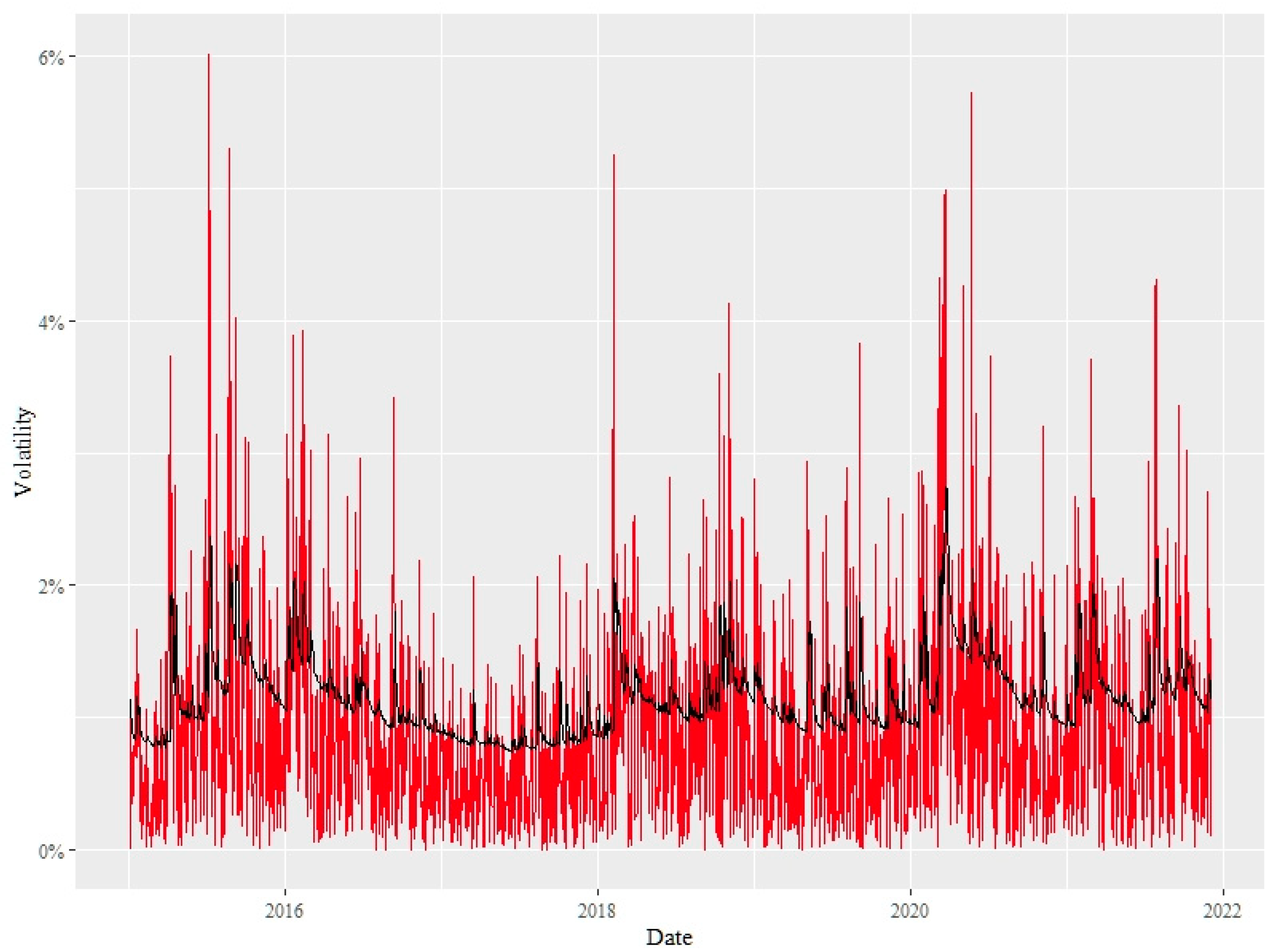
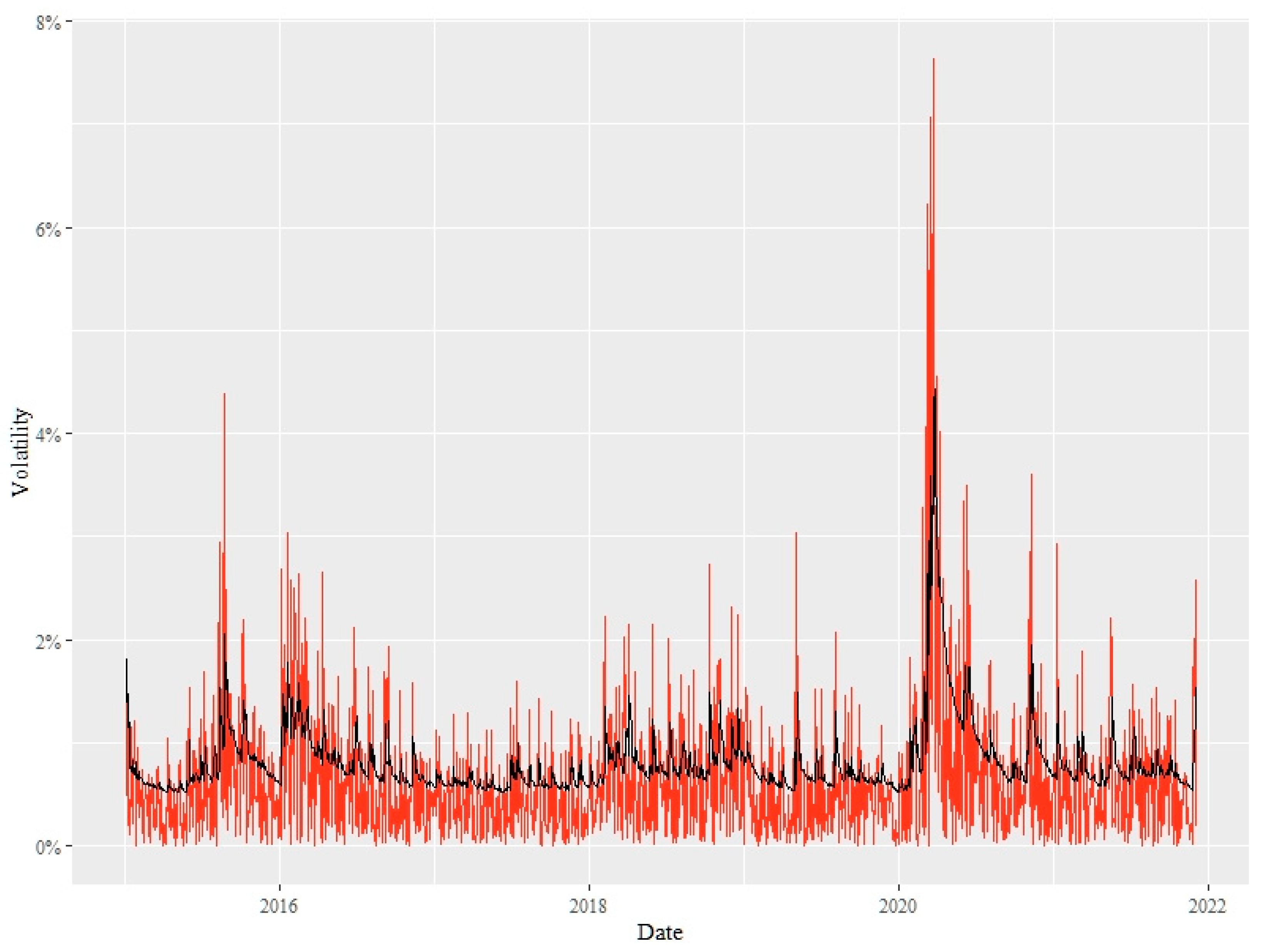
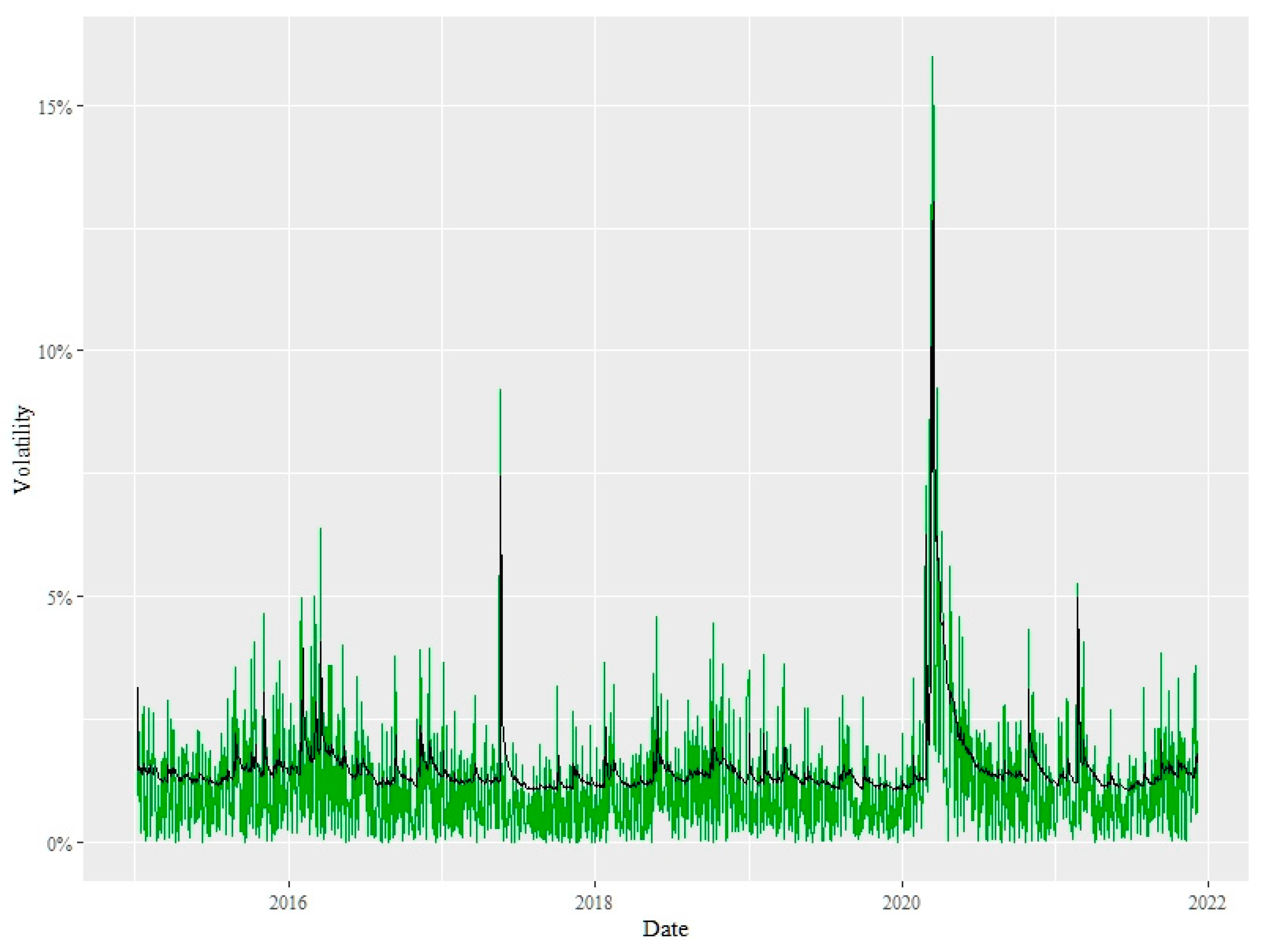
Daily data for the main stock market indexes of a sample of nine countries (three North American: Canada, the United States and Mexico; four Asian: Japan, Korea, Hong Kong and Singapore; and two South American: Brazil and Argentina) were retrieved from yahoo.finance.com (accessed on 10 December 2021). The data were first processed using a GARCH-M(1,1) model that captured the risk premium effect in two time periods (pre-COVID and COVID). To improve the flexibility of the model as well as the estimation of the coefficients, the residual generation process was assumed to have a NIG distribution, resulting in a skewed and leptokurtic version of the original specification. Furthermore, an MS GARCH(1,1) model with two regimes was estimated for the whole period.

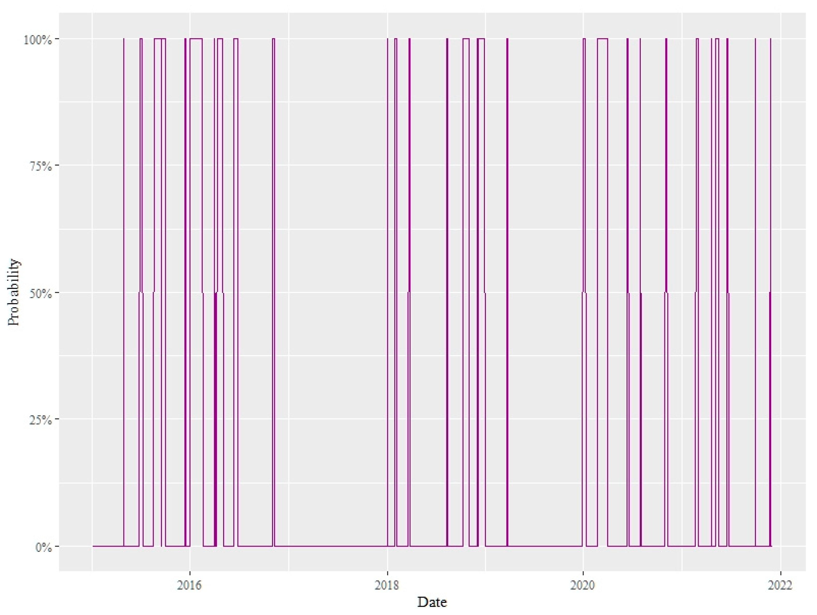
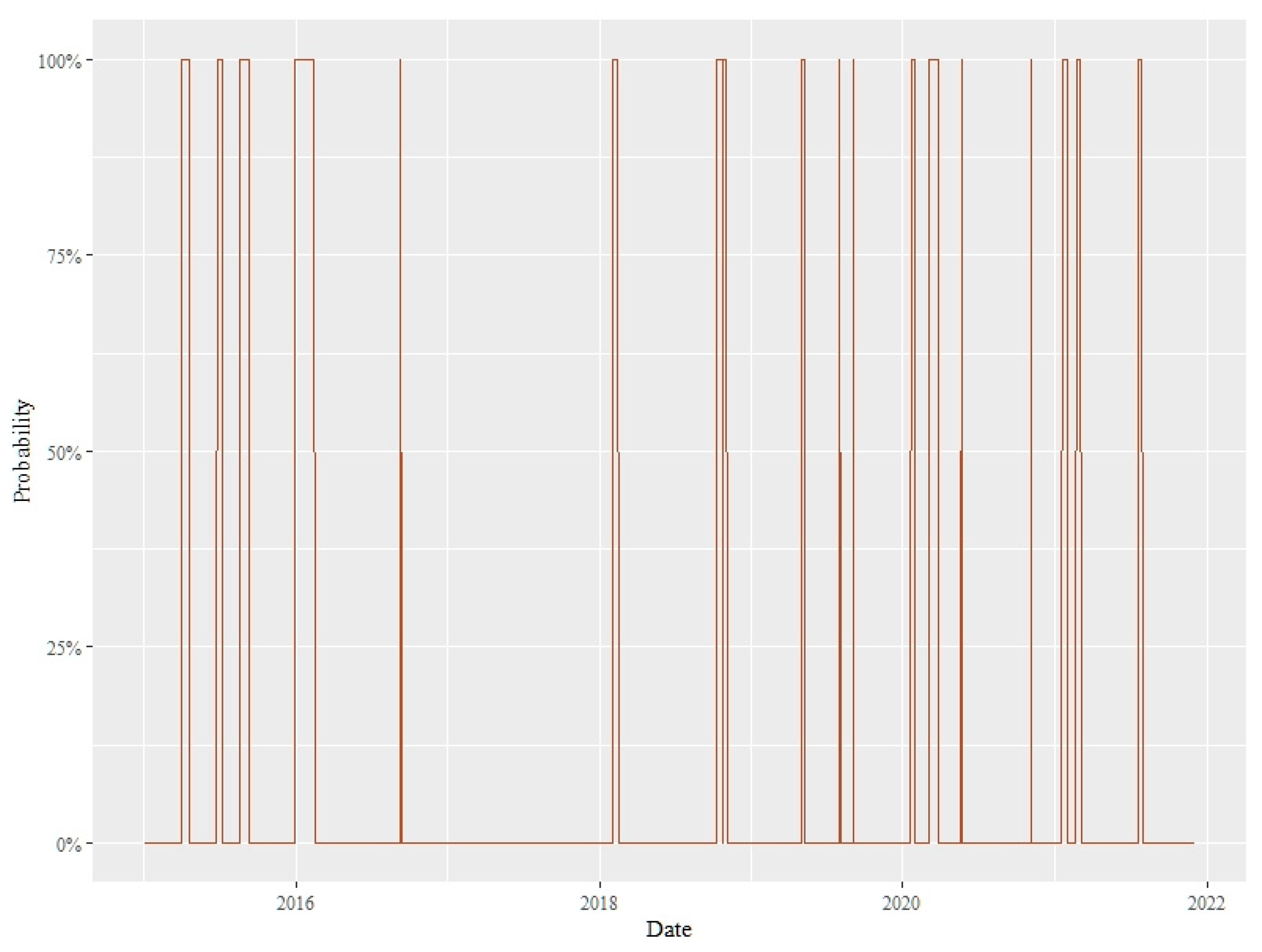
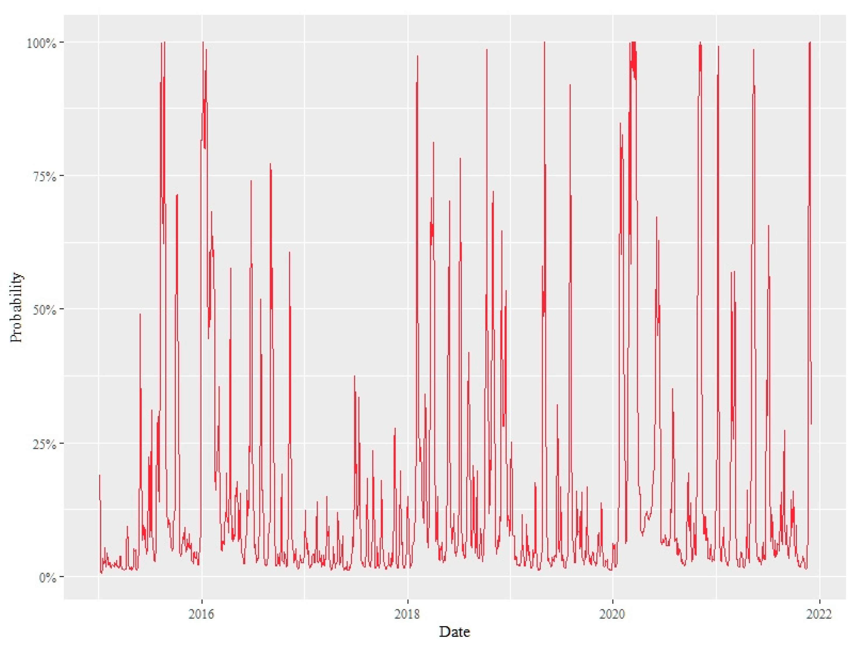
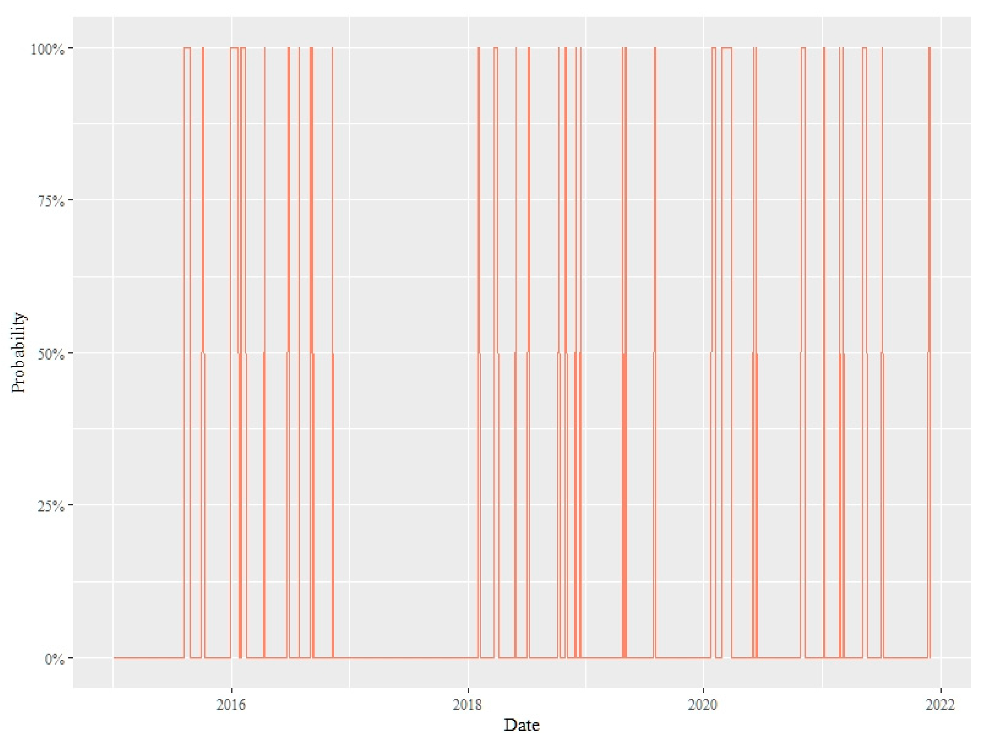
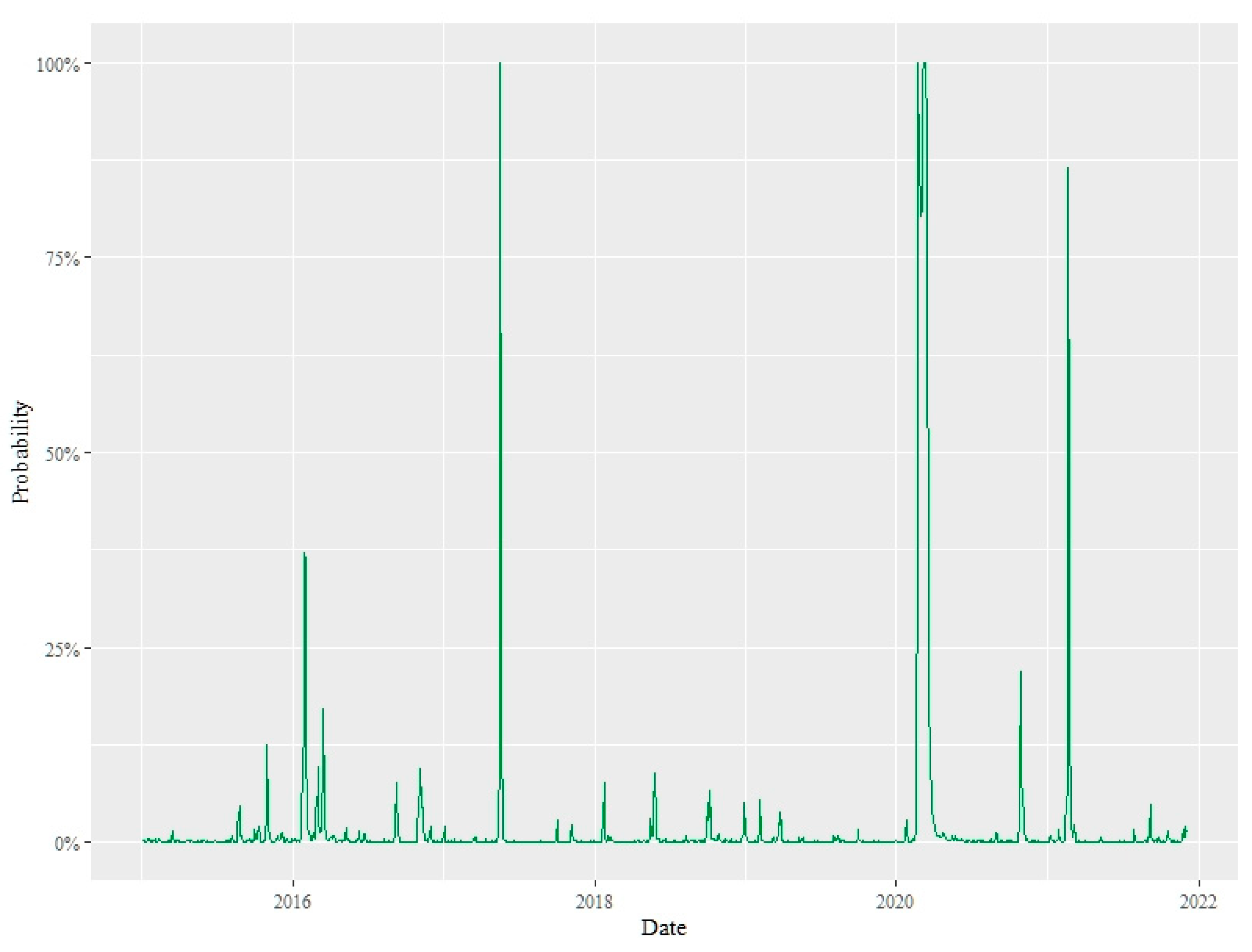
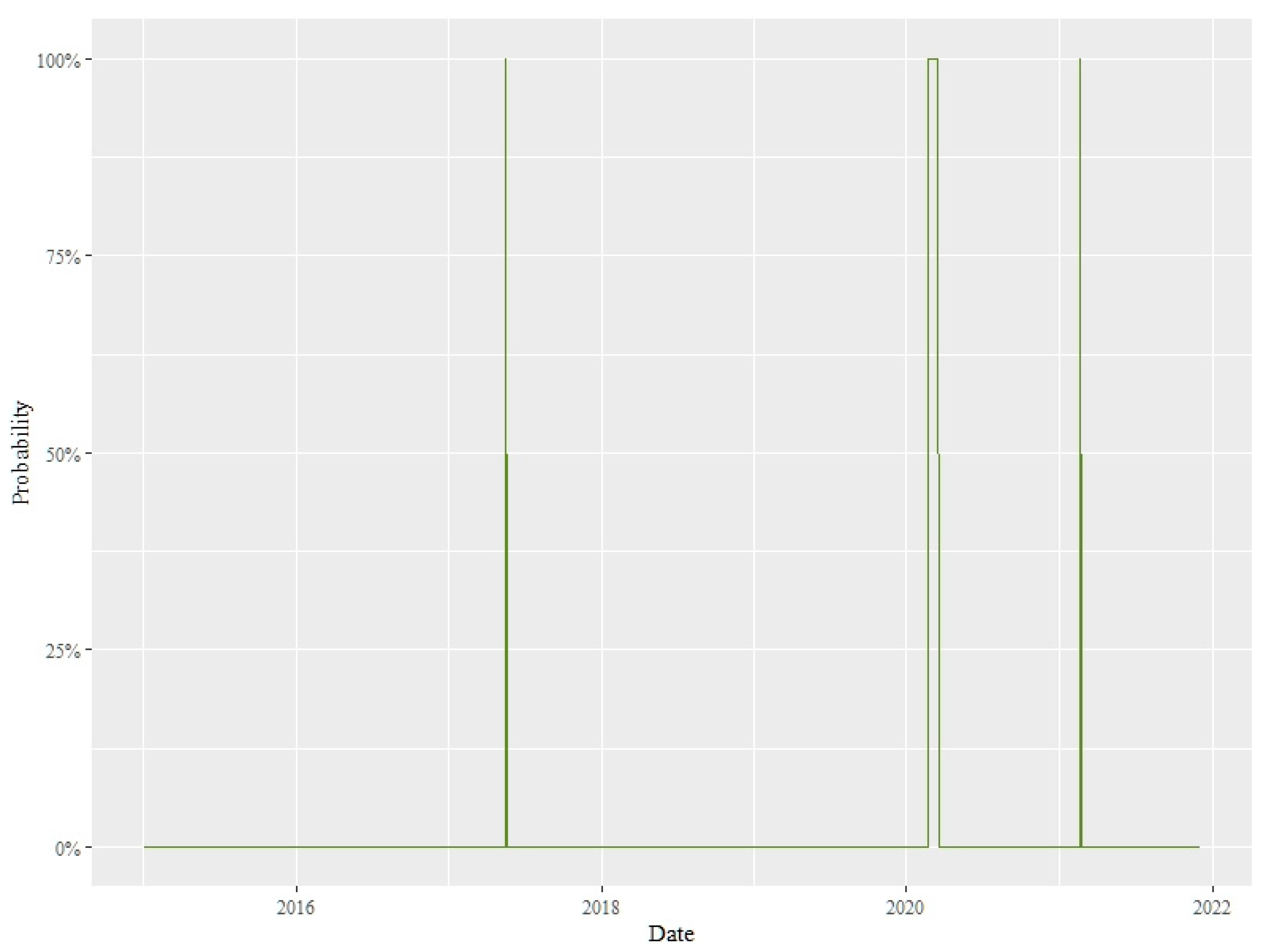
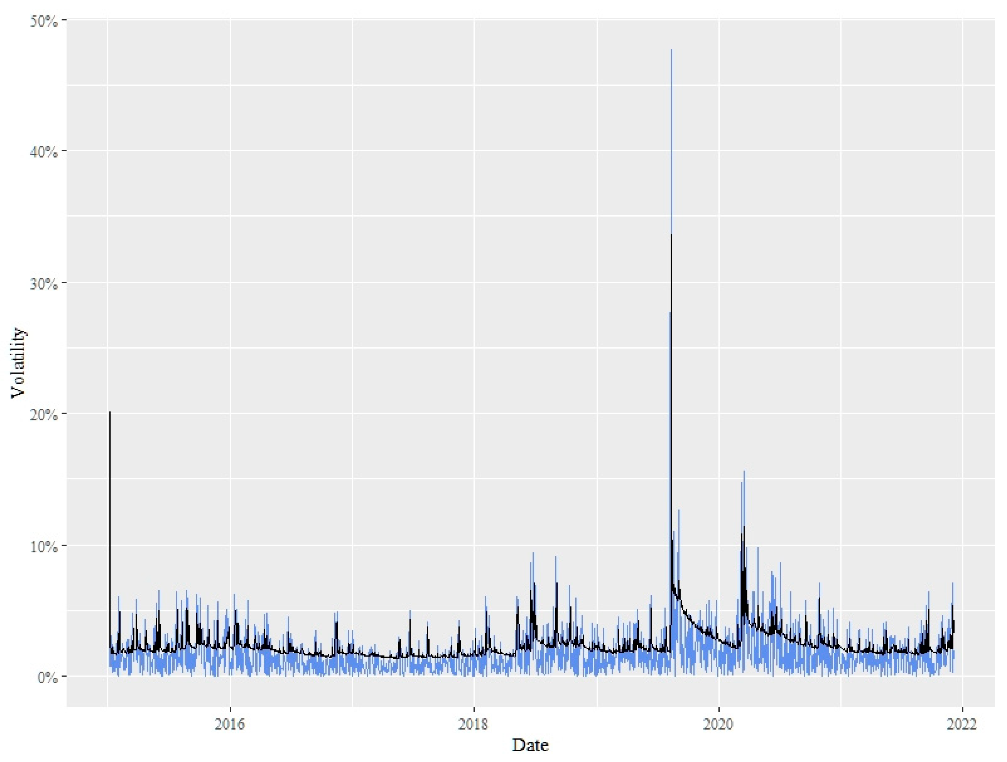
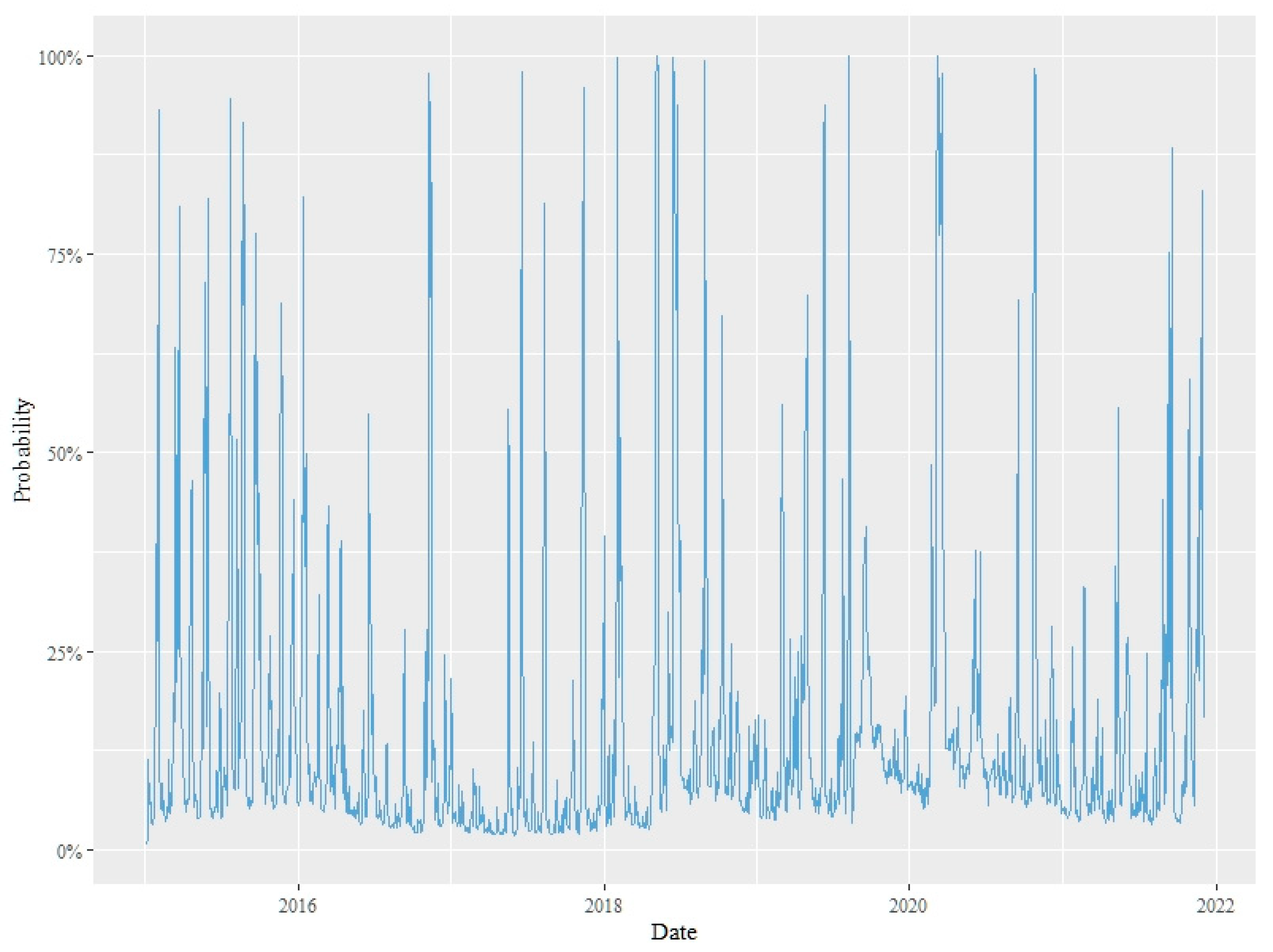
The results from the different models indicate that the stock markets from more developed countries experienced an important increase in their risk premium during the COVID period, likely attributable to the massive anticyclical economic government policies implemented. By contrast, developing countries, particularly those in Latin America, experienced a reduction and in some cases even a total loss of risk premium in their stock market indexes. This may be explained by a disproportional increase in volatility that could not be matched with the recovery of stock prices. However, the MS GARCH(1,1) results reveal that there was a double cause of that disproportional increase in volatility: the probability of transition from low and high volatility regimes was not large, and the unconditional probability to remain in the low volatility state was high. However, while the risk of a high volatility regime was modest, the volatility in either one of the two states was the highest in the sample.

Finally, the superiority of the MS GARCH(1,1) two-regime model over the simple GARCH and the three-regime models was confirmed based on the Akaike and Bayes Information Criteria (AIC and BIS), for all the national stock market results in our sample.

From the perspective of investors and portfolio risk managers, the identification of high and low volatility periods and their estimated probability of occurrence is useful for the characterization of stress scenarios and the design of emerging strategies. For governments and central bankers, the implementation of different policies should respond to the more likely scenarios but should also be prepared to respond to other less likely scenarios. Institutional preparedness to respond to as many different scenarios as may be identified with the use of MS GARCH models can make their interventions more successful. The COVID-19 pandemic experience has represented a laboratory to improve the understanding policy makers have of the role they are expected to play under extraordinary conditions. Although the approach presented in this work refers only to the stock market volatility and risk premium modeling, financial market stability is crucial to maintain high employment, economic growth, and productive chain functionality.

References

1. Pyun, J.H.; An, J. Capital and Credit Market Integration and Real Economic Contagion during the Global Financial Crisis. J. Int. Money Financ. 2016, 67, 172–193. [Google Scholar] [CrossRef]
2. Ahmad, R.; Etudaiye-Muhtar, O.F.; Matemilola, B.T.; Bany-Ariffin, A.N. Financial Market Development, Global Financial Crisis and Economic Growth: Evidence from Developing Nations. Port. Econ. J. 2016, 15, 199–214. [Google Scholar] [CrossRef] [Green Version]
3. Ahmad, W.; Sehgal, S.; Bhanumurthy, N.R. Eurozone Crisis and BRIICKS Stock Markets: Contagion or Market Interdependence? Econ. Model. 2013, 33, 209–225. [Google Scholar] [CrossRef]
4. Sansa, N.A. The Impact of the COVID-19 on the Financial Markets: Evidence from China and USA. Electron. Res. J. Soc. Sci. Humanit. 2020, 2, 29–39. [Google Scholar]
5. Hatmanu, M.; Cautisanu, C.; Ifrim, M. The Impact of Interest Rate, Exchange Rate and European Business Climate on Economic Growth in Romania: An ARDL Approach with Structural Breaks. Sustainability 2020, 12, 2798. [Google Scholar] [CrossRef] [Green Version]
6. Ozili, P.K.; Arun, T. Spillover of COVID-19: Impact on the Global Economy. SSRN Electron. J. 2020. [Google Scholar] [CrossRef] [Green Version]
7. Cortés, M.E.T.; Callejas, E.S. La Economía Mexicana: De La Recesión a La Depresión Ante La Pandemia de La COVID-19. J. Econ. Lit. JEL 2021, 18, 112–143. [Google Scholar]
8. Engle, R.F.; Lilien, D.M.; Robins, R.P. Estimating Time Varying Risk Premia in the Term Structure: The Arch-M Model. Econometrica 1987, 55, 391–407. [Google Scholar] [CrossRef]
9. Francq, C.; Zakoian, J.-M. GARCH Models: Structure, Statistical Inference and Financial Applications, 2nd ed.; John Wiley & Sons: Hoboken, NJ, USA, 2019; ISBN 9781119313564. [Google Scholar]
10. Yong, J.N.C.; Ziaei, S.M.; Szulczyk, K.R. The Impact of COVID-19 Pandemic on Stock Market Return Volatility: Evidence from Malaysia and Singapore. Asian Econ. Financ. Rev. 2021, 11, 191–204. [Google Scholar] [CrossRef]
11. Duttilo, P.; Gattone, S.A.; di Battista, T. Volatility Modeling: An Overview of Equity Markets in the Euro Area during COVID-19 Pandemic. Mathematics 2021, 9, 1212. [Google Scholar] [CrossRef]
12. Engle, R.F. Autoregressive Conditional Heteroscedacity with Estimates of Variance of United Kingdom Inflation. Econometrica 1982, 50, 987–1008. [Google Scholar] [CrossRef]
13. Bollerslev, T. Generalized Auroregressive Conditional Hetroskedasticity. J. Econom. 1986, 31, 307–327. [Google Scholar] [CrossRef] [Green Version]
14. Taylor, S.J. Modelling Financial Time Series; Wiley and Sons Ltd.: New York, NY, USA, 1986; ISBN 978-0471909934. [Google Scholar]
15. Glosten, L.R.; Jagannathan, R.; Runkle, D.E. On the Relation between the Expected Value and the Volatility of the Nominal Excess Return on Stocks. J. Financ. 1993, 48, 1779–1801. [Google Scholar] [CrossRef]
16. Nelson, D.B. Conditional Heteroskedasticity in Asset Returns: A New Approach. Econometrica 1991, 59, 347–370. [Google Scholar] [CrossRef]
17. Ding, Z.; Granger, C.W.J. Modeling Volatility Persistence of Speculative Returns: A New Approach. J. Econom. 1996, 73, 185–215. [Google Scholar] [CrossRef]
18. Adrian, T.; Rosenberg, J. Stock Returns and Volatility: Pricing the Short-Run and Long-Run Components of Market Risk. J. Financ. 2008, 63, 2997–3030. [Google Scholar] [CrossRef] [Green Version]
19. Engle, R.F.; Rangel, J.G. The Spline-GARCH Model for Low-Frequency Volatility and Its Global Macroeconomic Causes. Rev. Financ. Stud. 2008, 21, 1187–1222. [Google Scholar] [CrossRef]
20. Engle, R.F.; Ghysels, E.; Sohn, B. Stock Market Volatility and Macroeconomic Fundamentals. Rev. Econ. Stat. 2013, 95, 776–797. [Google Scholar] [CrossRef]
21. Amendola, A.; Candila, V.; Gallo, G.M. Choosing the Frequency of Volatility Components within the Double Asymmetric GARCH–MIDAS–X Model. Econom. Stat. 2021, 20, 12–28. [Google Scholar] [CrossRef]
22. Conrad, C.; Kleen, O. Two Are Better than One: Volatility Forecasting Using Multiplicative Component GARCH-MIDAS Models. J. Appl. Econom. 2020, 35, 19–45. [Google Scholar] [CrossRef] [Green Version]
23. Panorska, A.; Mittnik, S.; Rachev, S.T. Stable GARCH Models for Financial Time Series. Appl. Math. Lett. 1995, 8, 33–37. [Google Scholar] [CrossRef] [Green Version]
24. Barndorff-Nielsen, O.E. Processes of Normal Inverse Gaussian Type. Financ. Stoch. 1997, 2, 41–68. [Google Scholar] [CrossRef]
25. Forsberg, L.; Bollerslev, T. Bridging the Gap between the Distribution of Realized (ECU) Volatility and ARCH Modelling (of the Euro): The GARCH-NIG Model. J. Appl. Econom. 2002, 17, 535–548. [Google Scholar] [CrossRef]
26. Lamoureux, C.G.; Lastrapes, W.D. Persistence in Variance, Structural Change, and the GARCH Model. J. Bus. Econ. Stat. 1990, 8, 225. [Google Scholar] [CrossRef]
27. Hamilton, J.D. A New Approach to the Economic Analysis of Nonstationary Time Series and the Business Cycle. Econometrica 1989, 57, 357–384. [Google Scholar] [CrossRef]
28. Cai, J. A Markov Model of Switching-Regime ARCH. J. Bus. Econ. Stat. 1994, 12, 309. [Google Scholar] [CrossRef]
29. Hamilton, J.D.; Susmel, R. Autoregressive Conditional Heteroskedasticity and Changes in Regime. J. Econom. 1994, 64, 307–333. [Google Scholar] [CrossRef]
30. Ataurima Arellano, M.; Rodríguez, G. Empirical Modeling of High-Income and Emerging Stock and Forex Market Return Volatility Using Markov-Switching GARCH Models. N. Am. J. Econ. Financ. 2020, 52, 101163. [Google Scholar] [CrossRef]
31. Augustyniak, M. Maximum Likelihood Estimation of the Markov-Switching GARCH Model. Comput. Stat. Data Anal. 2014, 76, 61–75. [Google Scholar] [CrossRef]
32. Ardia, D.; Bluteau, K.; Boudt, K.; Catania, L.; Trottier, D.A. Markov-Switching GARCH Models in R: The MS GARCH Package. J. Stat. Softw. 2019, 91, 1–38. [Google Scholar] [CrossRef] [Green Version]
33. Sajjad, R.; Coakley, J.; Nankervis, J.C. Markov-Switching GARCH Modelling of Value-at-Risk. Stud. Nonlinear Dyn. Econ. 2008, 12, 1–29. [Google Scholar]
34. Su, J.B.; Hung, J.C. The Value-at-Risk Estimate of Stock and Currency-Stock Portfolios’ Returns. Risks 2018, 6, 133. [Google Scholar] [CrossRef] [Green Version]
35. Braione, M.; Scholtes, N.K. Forecasting Value-at-Risk under Different Distributional Assumptions. Econometrics 2016, 4, 3. [Google Scholar] [CrossRef] [Green Version]
36. Al Rahahleh, N.; Kao, R. Forecasting Volatility: Evidence from the Saudi Stock Market. J. Risk Financ. Manag. 2018, 11, 84. [Google Scholar] [CrossRef] [Green Version]
37. Naeem, M.; Tiwari, A.K.; Mubashra, S.; Shahbaz, M. Modeling Volatility of Precious Metals Markets by Using Regime-Switching GARCH Models. Resour. Policy 2019, 64, 101497. [Google Scholar] [CrossRef]
38. Shiferaw, Y.A.; Shiferaw, Y. The Bayesian MS-GARCH Model and Value-at-Risk in South African Agricultural Commodity Price Markets; International Association of Agricultural Economists: Toronto, ON, Canada, 2007. [Google Scholar]
39. De la Torre-Torres, O.V.; Galeana-Figueroa, E. A Test of Using Markov-Switching GARCH Models. Energies 2020, 2, 187–210. [Google Scholar]
40. Xiao, Y. Forecasting Extreme Risk Using Regime-Switching GARCH Models: A Case from an Energy Commodity. Int. J. Emerg. Mark. 2020, 16, 1556–1582. [Google Scholar] [CrossRef]
41. López-Herrera, F.; Mota-Aragón, M.B. Rendimiento y Volatilidades de Los Mercados Mexicanos Bursátil y Cambiario. Rev. Mex. Econ. Finanzas 2019, 14, 633–650. [Google Scholar] [CrossRef]
42. Zhang, Y.J.; Yao, T.; He, L.Y.; Ripple, R. Volatility Forecasting of Crude Oil Market: Can the Regime Switching GARCH Model Beat the Single-Regime GARCH Models? Int. Rev. Eco. Fin. 2019, 59, 302–317. [Google Scholar] [CrossRef]
43. Balcombe, K.; Fraser, I. Do Bubbles Have an Explosive Signature in Markov Switching Models? Econ. Model. 2017, 66, 81–100. [Google Scholar] [CrossRef]
44. Thies, S.; Molnár, P. Bayesian Change Point Analysis of Bitcoin Returns. Financ. Res. Lett. 2018, 27, 223–227. [Google Scholar] [CrossRef]
45. Ardia, D.; Bluteau, K.; Rüede, M. Regime Changes in Bitcoin GARCH Volatility Dynamics. Financ. Res. Lett. 2019, 29, 266–271. [Google Scholar] [CrossRef]
46. Caporale, G.M.; Zekokh, T. Modelling Volatility of Cryptocurrencies Using Markov-Switching GARCH Models. Res. Int. Bus. Financ. 2019, 48, 143–155. [Google Scholar] [CrossRef]
47. Ghorbel, A.; Jeribi, A. Contagion of COVID-19 Pandemic between Oil and Financial Assets: The Evidence of Multivariate Markov Switching GARCH Models. J. Investig. Compliance 2021, 22, 151–169. [Google Scholar] [CrossRef]
48. Urom, C.; Chevallier, J.; Zhu, B. A Dynamic Conditional Regime-Switching GARCH CAPM for Energy and Financial Markets. Energy Econ. 2020, 85, 104577. [Google Scholar] [CrossRef]
49. Mohammadi, H.; Tan, Y. Return and Volatility Spillovers across Equity Markets in Mainland China, Hong Kong and the United States. Econometrics 2015, 3, 215–232. [Google Scholar] [CrossRef] [Green Version]
50. Akhtaruzzaman, M.; Boubaker, S.; Sensoy, A. Financial Contagion during COVID–19 Crisis. Financ. Res. Lett. 2021, 38, 101604. [Google Scholar] [CrossRef] [PubMed]
51. Demir, E.; Kizys, R.; Rouatbi, W. COVID-19 Vaccinations and the Volatility of Energy Companies in International Markets. J. Risk Financ. Manag. 2021, 14, 611. [Google Scholar] [CrossRef]
52. Alexakis, C.; Eleftheriou, K.; Patsoulis, P. COVID-19 Containment Measures and Stock Market Returns: An International Spatial Econometrics Investigation. J. Behav. Exp. Financ. 2021, 29, 100428. [Google Scholar] [CrossRef] [PubMed]
53. Scherf, M.; Matschke, X.; Rieger, M.O. Stock Market Reactions to COVID-19 Lockdown: A Global Analysis. Financ. Res. Lett. 2021, 45, 102245. [Google Scholar] [CrossRef]
54. Fernandez-Perez, A.; Gilbert, A.; Indriawan, I.; Nguyen, N.H. COVID-19 Pandemic and Stock Market Response: A Culture Effect. J. Behav. Exp. Financ. 2021, 29, 100454. [Google Scholar] [CrossRef]
55. Haldar, A.; Sethi, N. The News Effect of COVID-19 on Global Financial Market Volatility. Bul. Ekon. Monet. Dan Perbank. 2021, 24, 33–58. [Google Scholar] [CrossRef]
56. Ozkan, O. Impact of COVID-19 on Stock Market Efficiency: Evidence from Developed Countries. Res. Int. Bus. Financ. 2021, 58, 101445. [Google Scholar] [CrossRef]
57. Szczygielski, J.J.; Bwanya, P.R.; Charteris, A.; Brzeszczyński, J. The Only Certainty Is Uncertainty: An Analysis of the Impact of COVID-19 Uncertainty on Regional Stock Markets. Financ. Res. Lett. 2021, 43, 101945. [Google Scholar] [CrossRef] [PubMed]
58. Nian, R.; Xu, Y.; Yuan, Q.; Feng, C.; Lendasse, A. Quantifying Time-Frequency Co-Movement Impact of COVID-19 on U.S. and China Stock Market Toward Investor Sentiment Index. Front. Public Health 2021, 9, 727047. [Google Scholar] [CrossRef]
59. Chiang, T.C. Evidence of Economic Policy Uncertainty and COVID-19 Pandemic on Global Stock Returns. J. Risk Financ. Manag. 2022, 15, 28. [Google Scholar] [CrossRef]
60. Setiawan, B.; ben Abdallah, M.; Fekete-Farkas, M.; Nathan, R.J.; Zeman, Z. GARCH (1,1) Models and Analysis of Stock Market Turmoil during COVID-19 Outbreak in an Emerging and Developed Economy. J. Risk Financ. Manag. 2021, 14, 576. [Google Scholar] [CrossRef]
61. Yousaf, I.; Bouri, E.; Ali, S.; Azoury, N. Gold against Asian Stock Markets during the COVID-19 Outbreak. J. Risk Financ. Manag. 2021, 14, 186. [Google Scholar] [CrossRef]
62. Manuj, H. Is Gold a Hedge against Stock Price Risk in US. or Indian Markets? Risks 2021, 9, 174. [Google Scholar] [CrossRef]
63. Nieto, B.; Rubio, G. The Effects of the COVID-19 Crisis on Risk Factors and Option-Implied Expected Market Risk Premia: An International Perspective. J. Risk Financ. Manag. 2022, 15, 13. [Google Scholar] [CrossRef]
64. Bizuneh, M.; Geremew, M. Assessing the Impact of COVID-19 Pandemic on Emerging Market Economies’ (EMEs) Sovereign Bond Risk Premium and Fiscal Solvency. East. Econ. J. 2021, 47, 519–545. [Google Scholar] [CrossRef]
65. Ngunyi, A.; Mundia, S.; Omari, C. Modelling Volatility Dynamics of Cryptocurrencies Using GARCH Models. J. Math. Financ. 2019, 9, 591–615. [Google Scholar] [CrossRef] [Green Version]
66. Cerqueti, R.; Giacalone, M.; Mattera, R. Skewed Non-Gaussian GARCH Models for Cryptocurrencies Volatility Modelling. Inf. Sci. 2020, 527, 1–26. [Google Scholar] [CrossRef]
67. Jensen, M.B.; Lunde, A. The NIG-S&ARCH Model: A Fat-Tailed, Stochastic, and Autoregressive Conditional Heteroskedastic Volatility Model. Econom. J. 2001, 4, 319–342. [Google Scholar] [CrossRef]
68. Cont, R. Empirical Properties of Asset Returns: Stylized Facts and Statistical Issues. Quant. Financ. 2001, 1, 223–236. [Google Scholar] [CrossRef]
69. Barndorff-Nielsen, O.E. Normal Inverse Gaussian Distributions and Stochastic Volatility Modelling. Scand. J. Stat. 1997, 24, 1–13. [Google Scholar] [CrossRef]
70. Andersson, J. On the Normal Inverse Gaussian Stochastic Volatility Model. J. Bus. Econ. Stat. 2001, 19, 44–54. [Google Scholar] [CrossRef]
71. Barndorff-Nielsen, O.E.; Shepard, N. Non-Gaussian Ornstein-Uhlenbeck-Based Models and Some of Their Uses in Financial Economics. J. R. Stat. Soc. Ser. B Stat. Methodol. 2001, 63, 167–241. [Google Scholar] [CrossRef]
72. Albrecher, H.; Predota, M. On Asian Option Pricing for NIG Lévy Processes. J. Comput. Appl. Math. 2004, 172, 153–168. [Google Scholar] [CrossRef] [Green Version]
73. Haas, M. A New Approach to Markov-Switching GARCH Models. J. Financ. Econom. 2004, 2, 493–530. [Google Scholar] [CrossRef]
74. Katsiampa, P. Volatility Estimation for Bitcoin: A Comparison of GARCH Models. Econ. Lett. 2017, 158, 3–6. [Google Scholar] [CrossRef] [Green Version]
75. Fiszeder, P.; Perczak, G. Low and High Prices Can Improve Volatility Forecasts during Periods of Turmoil. Int. J. Forecast. 2016, 32, 398–410. [Google Scholar] [CrossRef]
Figure 1. Volatility (in color) and unconditional estimation (in black) of the MS GARCH(1,1) model: Mexico.
Mathematics 10 01353 g001
Figure 2. Smooth probabilities for state 2 MS GARCH(1,1): Mexico.
Mathematics 10 01353 g002
Figure 3. Corner probabilities with 50% threshold value to be in state 2: Mexico.
Mathematics 10 01353 g003
Figure 4. Volatility (in color) and unconditional estimation (in black) of the MS GARCH(1,1) model: United States.
Mathematics 10 01353 g004
Figure 5. Smooth probabilities for state 2 MS GARCH(1,1): United States.
Mathematics 10 01353 g005
Figure 6. Corner probabilities with 50% threshold value to be in state 2 USA.
Mathematics 10 01353 g006
Figure 7. Volatility (in color) and unconditional estimation (in black) of the MS GARCH(1,1) model: Canada.
Mathematics 10 01353 g007
Figure 8. Smooth probabilities for state 2 MS GARCH(1,1): Canada.
Mathematics 10 01353 g008
Figure 9. Corner probabilities with 50% threshold value to be in state 2: Canada.
Mathematics 10 01353 g009
Figure 10. Volatility (in color) and unconditional estimation (in black) of the MS GARCH(1,1) model: South Korea.
Mathematics 10 01353 g010
Figure 11. Smooth probabilities for state 2 MS GARCH(1,1): South Korea.
Mathematics 10 01353 g011
Figure 12. Corner probabilities with 50% threshold value to be in state 2: South Korea.
Mathematics 10 01353 g012
Figure 13. Absolute volatilities and unconditional estimation of MS GARCH(1,1): Japan.
Mathematics 10 01353 g013
Figure 14. Smooth probabilities for state 2 MS GARCH(1,1): Japan.
Mathematics 10 01353 g014
Figure 15. Corner probabilities with 50% threshold value to be in state 2: Japan.
Mathematics 10 01353 g015
Figure 16. Volatility (in color) and unconditional estimation (in black) of MS GARCH(1,1) model: Hong Kong.
Mathematics 10 01353 g016
Figure 17. Smooth probabilities for state 2 MS GARCH(1,1): Hong Kong.
Mathematics 10 01353 g017
Figure 18. Corner probabilities with 50% threshold value to be in state 2: Hong Kong.
Mathematics 10 01353 g018
Figure 19. Volatility (in color) and unconditional estimation (in black) of MS GARCH(1,1) model: Singapore.
Mathematics 10 01353 g019
Figure 20. Smooth probabilities for state 2 MS GARCH(1,1): Singapore.
Mathematics 10 01353 g020
Figure 21. Corner probabilities with 50% threshold value to be in state 2: Singapore.
Mathematics 10 01353 g021
Figure 22. Volatility (in color) and unconditional estimation (in black) of MS GARCH(1,1) model: Brazil.
Mathematics 10 01353 g022
Figure 23. Smooth probabilities for state 2 MS GARCH(1,1): Brazil.
Mathematics 10 01353 g023
Figure 24. Corner probabilities with 50% threshold value to be in state 2: Brazil.
Mathematics 10 01353 g024
Figure 25. Volatility (in color) and unconditional estimation (in black) of MS GARCH(1,1) model: Argentina.
Mathematics 10 01353 g025
Figure 26. Smooth probabilities for state 2 MS GARCH(1,1): Argentina.
Mathematics 10 01353 g026
Figure 27. Corner probabilities with 50% threshold value to be in state 2: Argentina.
Mathematics 10 01353 g027