Inverse Analysis for the Convergence-Confinement Method in Tunneling

Abstract

For the safety of tunnel excavation, the observation of tunnel convergence not only provides a technique for assessing the stability of the surrounding ground, but also provides an estimate of the constitutive parameters of geological materials. This estimation method belongs to an inverse algorithm process called the inverse calculation method (ICM), which utilizes the incremental concept in the convergence-confinement method (CCM) to solve the support-ground interaction of circular tunnel excavation. The method is to determine the mathematical solution of the intersection of the two nonlinear curves, the support confining curve (SCC) and the ground reaction curve (GRC) in the CCM by using Newton’s recursive method and inversely calculating the unknown parameters. To verify the validity of the developed inverse algorithm process, this study compares the results of the ICM with those of the published articles. In addition, the modulus of rock mass and unsupported span are inversely deduced using the values of convergence difference measured in the practical case of railway tunnels.

1. Introduction

The inverse analysis is formulated to determine the constitutive coefficients of geo-material that minimize the difference between the experimentally measured values and the calculated data. The observation method in engineering practice is to use an arranged monitoring system, which can observe the changing trend of geo-material behavior. This is a key point when designing tunnel supports [1,2]. The use of measurements can reveal important aspects of support-ground interactions and predictions of tunnel surrounding rock behavior. The back analysis involves a process in which the different parameters and assumptions of the test problem are changed so that the analysis results match the predicted performance as much as possible [3,4,5,6]. A displacement-based back analysis methodology is used which yields the complete initial stress and Young’s modulus of the rock mass by assuming the rock as linearly elastic and isotropic [7,8,9]. In addition, many researchers have studied the inverse calculation of in situ stress in rock mass using different search algorithms [10,11,12], and also many articles concerning the inverse elastic scattering problem and inverse conductivity problem are included in the literature review in the field of inverse analysis [13,14,15].

The Convergence-Confinement Method (CCM) is a useful preliminary tool for support design often used in tunnel engineering. Many studies discuss its application in predicting and analyzing the behavior of underground structures with supports [16,17,18,19,20]. The method consists of three different curves: the confinement loss curve (CLC), the support confining curve (SCC), and the ground reaction force curve (GRC), combined with simulating the interaction behavior of support-ground, as shown in Figure 1 [21]. As the tunnel excavation progresses, changes in surrounding rock stress lead to a concomitant increase in radial displacement; therefore, the GRC plays an important role in determining when to install support and the stiffness of that support [22,23]. The SCC characterizes the support deformation caused by the mobilized support pressure exerted on it, and the mobilized support pressure that can be tolerated by radial convergence that occurs after support is installed, as well as the support stiffness employed [24,25,26]. As shown in the upper part of Figure 1, the third curve of this method is called the confinement loss curve (CLC) [27]. This curve represents a radial displacement line along the excavation direction of the tunnel which can be represented by a mathematical function through regression analysis. The purpose is to use this function to explain the simulation of stress relief due to the distance between the observed section and the advancing working face [16,27]. In recent studies, some different views and suggestions have been expressed regarding the definition and assumptions of confinement loss in CCM analysis [28,29]. An original study is to use a value of confinement loss to represent the percentage of reverse stress removal at the intrados of the excavation face, thereby simulating the degree of stress change between the tunnel face and the observed section, and its value is between 0 and 1 [16].

The explicit algorithm process proposed by this paper is used to solve the stress/displacement of support-ground interaction in the analysis of CCM with the concept of increment, and can be realized by transforming the analytical solutions to an executable computation that can be directly calculated by using a computation spreadsheet (e.g., the Microsoft Excel format). This feature of the procedure, the so-called the explicit analysis method (EAM), consists of two characteristics, the direct calculation method (DCM) and the inverse calculation method (ICM), as shown in Figure 2.

Firstly, the forward analysis of the so-called direct calculation method (DCM), can solve with the solutions for the interaction between GRC and SCC in the equilibrium state. The unknown values are the plastic zone radius, the radial displacement, and the mobilized support pressure. The DCM with the explicit procedure can deal with using the confinement loss as an incremental step to simulate the effect of advance excavation of the tunnel face, calculating the stresses and displacements in each step including those at the points A, B, C (or D) and E, as shown in Figure 1.

Secondly, the backward analysis of the so-called inverse calculation method (ICM) applies the convergence difference (e.g., the difference in tunnel convergence) as a known parameter to estimate the unknown parameters, such as the modulus of rock mass (E_m) and the unsupported span (d). In the inverse algorithm process, the intersection of GRC and SCC is the solution we want. In the elastic region, we use simultaneous equations to find the solution of the two straight lines, and apply Newton’s recursive method to find the solution of the two curves in the plastic region.

The objective of this paper is to provide concepts of inverse analysis (ICM) for the Convergence-Confinement approach in tunneling and presents a comprehensive discussion on the solutions for the interaction of support-ground in the equilibrium state for the support design and on the estimation of the modulus of rock mass and the unsupported span. It provides the full set of equations and the details of their derivation, flowchart of calculation, verification, and the comparison with the published research results of Oreste (2009) [19], Rocksupport (2004) [20] and Gschwandtner-Galler (2012) [26]. Moreover, the study on inverse analysis is concluded with the application of one of the suggested methods in the case of railway tunnels.

2. Problem Description

2.1. Relationship between Confinement Loss and Unsupported Span

In the process of tunnel excavation, the changes in stress and displacement caused by the continuous excavation of the tunnel at some measuring points of the observation section can be described by the influence of the excavation of the tunnel face. In addition, the convergence measurement at a certain location is the relative displacement of measurement points at the intrados of the tunnel. At a certain distance (z) to the working face, the definition of confinement loss (λ_z) can be given as [27]:

$${\lambda }_z={\lambda }_d+\left(1-{\lambda }_d\right)f\left(z/R\right),$$

(1)

where λ_d is the confinement loss at the unsupported distance (d) to the working face, and R is the tunnel excavation radius. The advancing effect function, f(z/R), is supposed by the hyperbolic function that contains only one variable and can be represented as

$$f\left((z-d)/R\right)=1-{\left(\frac{m}{m+(z-d)/R}\right)}^2,$$

(2)

where the parameter of the function (m) can be found by the regression analysis with the tunnel convergence data, and λ_d is a confinement loss at the unsupported distance (d) to the working face, and can be suggested as the following:

$${\lambda }_d=1-{\left(\frac{m}{m+(d/R)}\right)}^4$$

(3)

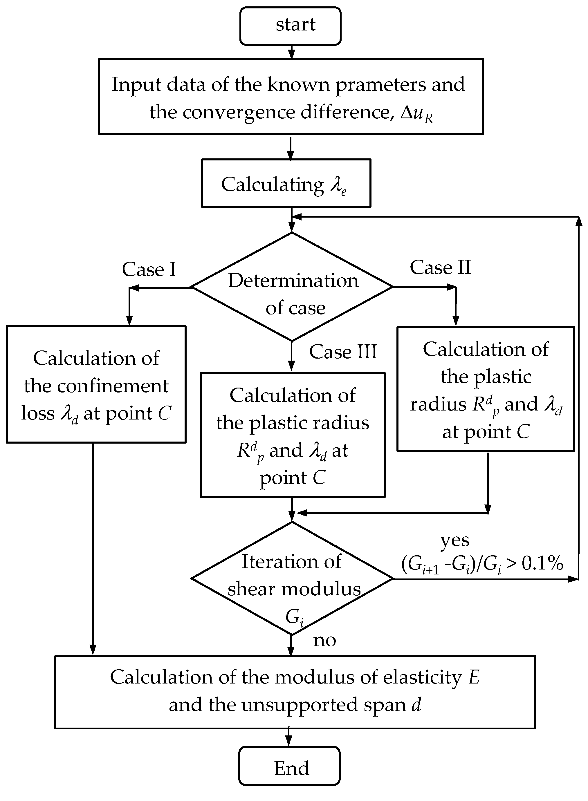
2.2. Explicit Algorithm Process of the Inverse Calculation Method (ICM)

As shown in Figure 3, the inverse algorithm process is used in the analysis of ICM. According to the objective functions that define the objective of the optimization, an objective function is a single scalar value that is formulated from a set of design responses. In this study, the design responses including the modulus of rock mass and unsupported span are defined from the solution of GRC and SCC in the equilibrium state. The objective function could be minimized by using the iteration of the design responses. In addition, as a constraint that imposes limitations on the optimization and defines a feasible design, the modulus of rock mass (E) is used as an objective function. We apply a constraint that uses the initial value (E_i) used by the DCM, where the optimization module is forced to seek an optimum solution that both optimizes the modulus of rock mass objective and satisfies the constraint. The unknown parameters considered in this study are the modulus of rock mass (e.g., the shear modulus, G, or the modulus of elasticity, E) and the unsupported span (d). The input data includes the parameters of the geometry of the tunnel, the properties of the material, the stress condition, etc., and the specific known parameters such as the convergence difference (Δu_R), which is a difference of the radial displacement between point C and point E. One must be aware that the first step of calculation in ICM is to use the input data of DCM containing the initial modulus of rock mass, and the second step of the calculation is to use the iteration algorithms to find a convergence value of the modulus of rock mass. Similarly, for another unknown parameter, the unsupported span can also be obtained by the same iteration algorithms.

As shown in Figure 1, from the moment of installing support (point C or D) to the equilibrium state (point E), the stresses of the ground in the elastic or the plastic regions can be distinguished by using the difference between the confinement loss in the elastic limit state (λ_e) and that in the equilibrium state (λ_s). In other words, if λ_s < λ_e, it means that the stresses in the equilibrium state are in the elastic region, otherwise λ_e < λ_s, those are in the plastic region. To distinguish whether the stress at the points C and E are in the elastic or the plastic regions, as shown in Figure 3, this study presents three analysis situations that include the stress state of points C and E, which are (1) both in the elastic region (Case I, λ_d < λ_s < λ_e), (2) in the elastic and plastic regions, respectively (Case II, λ_d < λ_e < λ_s), and (3) both in the plastic region (Case III, λ_e < λ_d < λ_s). In this case (III) and in a certain i step (for i = 1 to n, i is an incremental step in the recursion), for finding the plastic radius at the moment of installing support (point C) and in the final equilibrium situation (point E) respectively, it is also necessary to assume considering an initial shear modulus of rock mass (G_i) which is suitable to be calculated for the first i step of recursion by the direct calculation method (DCM), and after once a calculation completed, then one can obtain the new shear modulus of rock mass in the i + 1 step, (G_i+1), which can be used in the next step of calculation for (R_p^d)_i+1 and (R_p^s)_i+1. This process can be continuously repeated until a difference of the value of G between step i + 1 and step i is less than the small accuracy value (ε), which is equal to 0.01%. Therefore, the process of calculation is performed, and the shear modulus of rock mass can be obtained in this case. The modulus of rock mass (E_m) can be estimated from the shear modulus using the classic relationship from isotropic elasticity,

E_m = 2G(1 + ν)

(4)

3. Equations Derivation of the Inverse Calculation Method (ICM)

3.1. Support-Ground Interaction Occurred in the Elastic State

The intersection between GRC and SCC allows one to obtain the mobilized support pressure (P_s) that acts on the supports and the radial displacement (u_R^s) of the tunnel in the equilibrium state. In the analysis procedure of ICM, the equation for the SCC can be represented as:

$$P_s=k_s^{}\left(\frac{\Delta u_R}{R}\right),$$

(5)

where k_s is the stiffness of the support, Δu_R is a difference of the radial displacement between point C (u_R^d) and point E (u_R^s), that is, the convergence after support installation, and can be shown as

$$\Delta u_R=\left(u_R^s-u_R^d\right)$$

(6)

where the superscript letters d and s indicate the locations of points C and E, respectively. For dimensionless, the convergence difference (Δu_R) can be normalized by (2G/σ_v) and rearranged as

$$\frac{2G}{{\sigma }_v}\left(\frac{\Delta u_R}{R}\right)=\frac{2G}{{\sigma }_v}\frac{p_s}{k_s^{}}$$

(7)

where σ_v is the vertical overburden stress.

(1) Case I: The stress state of points C and E are both in the elastic region (Figure 1). The convergence difference (Δu_R) can be obtained by the following:

$$\frac{2G}{{\sigma }_v}\left(\frac{\Delta u_R}{R}\right)==\left({\lambda }_s-{\lambda }_d\right)$$

(8)

Therefore, the difference of confinement loss between point C and point E can be described as

$$\left({\lambda }_s-{\lambda }_d\right)=\frac{1-{\lambda }_d}{1+\frac{k_s^{}}{2G^{}}}$$

(9)

For the unknown parameter, the shear modulus of rock mass (G), can be obtained by the following:

$$2G=\frac{\left(1-{\lambda }_d\right){\sigma }_v}{\left(\frac{\Delta u_R}{R}\right)}-k_s,$$

(10)

In addition, rearranging the above equation for the unknown parameter, the confinement loss of the unsupported span (λ_d), can be obtained as follow:

$${\lambda }_d=1-\left(\frac{2G+k_s}{{\sigma }_v}\right)\left(\frac{\Delta u_R}{R}\right)$$

(11)

3.2. Support-Ground Interaction Occurred in the Plastic State

When the stresses of the ground wall in the equilibrium state (point E) are in the plastic region, two conditions of the stress state exist at the moment of installing the support (point C), which are in the elastic region (Case II) and the plastic region (Case III). Both cases of the support point are described by the following representations.

(2) Case II: The stress state of points C and E are in the elastic and plastic regions, respectively. Equation (6) can be normalized by (2G/σ_vR) and rearranged as

$$\frac{2G}{{\sigma }_v}\left(\frac{\Delta u_R}{R}\right)=\frac{2G}{{\sigma }_v}\left(\frac{u_R^s}{R}\right)-\frac{2G}{{\sigma }_v}\left(\frac{u_R^d}{R}\right),$$

(12)

For the unknown parameter, the shear modulus of rock mass (G), can be obtained by the following:

$$2G=\frac{{\sigma }_v}{\left(\frac{\Delta u_R}{R}\right)}\left[{\lambda }_e\left[C_1+C_2{\left(\frac{R}{R_p^s}\right)}^{K_p-1}+C_3{\left(\frac{R_p^s}{R}\right)}^{K_{\psi }+1}\right]-{\lambda }_d\right]$$

(13)

where λ_d is a confinement loss at the unsupported distance (d) to the working face, and the radial displacement (u_R^s) of the tunnel in the equilibrium state can be given as the following, respectively.

$$\frac{2G}{{\sigma }_v}\frac{u_R^d}{R}={\lambda }_d$$

(14)

$$\frac{2G}{{\sigma }_o}\frac{u_R^s}{R}={\lambda }_e\left[C_1+C_2{\left(\frac{R}{R_p^s}\right)}^{K_p-1}+C_3{\left(\frac{R_p^s}{R}\right)}^{K_{\psi }+1}\right]$$

(15)

where C₁, C₂, and C₃ are the coefficients of rock mass, K_p is the coefficient of the lateral passive pressure, K_ψ is the coefficient of the plastic flow, ψ is the dilation angle of the rock mass, and the confinement loss in the elastic limit state (λ_e) is a function of the peak strength parameters of rock mass (the cohesion c and the internal friction angle φ) and can be given as

$${\lambda }_e=\frac{(K_p-1)+2N}{(K_p+1)},$$

(16)

where the stability number N equals σ_c/2σ_v, and σ_c is the uniaxial compression strength (UCS) of rock mass. The plastic zone radius in the equilibrium state (R_p^s) can be found by applying Newton’s recursive method and given as

$${\left(\frac{R_p^s}{R}\right)}_{n+1}={\left(\frac{R_p^s}{R}\right)}_n-\frac{f\left({\left(\frac{R_p^s}{R}\right)}_n\right)}{f\prime \left({\left(\frac{R_p^s}{R}\right)}_n\right)}$$

(17)

where ƒ′(R_p^s/R) denotes the derivative of the function ƒ(R_p^s/R), and n is the incremental step in the recursion and can be shown as

$$f\left(\frac{R_p^s}{R}\right)=\left[C_2-\frac{4G}{k_s\left(K_p-1\right)}\right]{\left(\frac{R_p^s}{R}\right)}^{1-K_p}+C_3{\left(\frac{R_p^s}{R}\right)}^{K_{\psi }+1}-\left[C_2{\left(\frac{R}{R_p^d}\right)}^{K_p-1}+C_3{\left(\frac{R_p^d}{R}\right)}^{K_{\psi }+1}\right]-\frac{4GN}{{\lambda }_e{k}_s\left(K_p-1\right)}$$

(18)

$$f^{\prime }\left(\frac{R_p^s}{R}\right)=\left[C_2-\frac{4G}{k_s\left(K_p-1\right)}\right]\left(1-K_p\right){\left(\frac{R_p^s}{R}\right)}^{-K_p}+C_3\left(K_{\psi }+1\right){\left(\frac{R_p^s}{R}\right)}^{K_{\psi }}$$

(19)

In addition, rearranging the above equation for the unknown parameter, the confinement loss of the unsupported span (λ_d) can be obtained as follows:

$${\lambda }_d={\lambda }_e\left[C_1+C_2{\left(\frac{R}{R_p^s}\right)}^{K_p-1}+C_3{\left(\frac{R_p^s}{R}\right)}^{K_{\psi }+1}\right]-\left(\frac{2G}{{\sigma }_v}\frac{\Delta u_R}{R}\right),$$

(20)

(3) Case III: The stress state of points C and E are both in the plastic region (Figure 1). The shear modulus of rock mass can be obtained by the following:

$$2G=\frac{{\lambda }_e{\sigma }_v}{\left(\frac{\Delta u_R}{R}\right)}\left[\left(C_2{\left(\frac{R}{R_p^s}\right)}^{K_p-1}+C_3{\left(\frac{R_p^s}{R}\right)}^{K_{\psi }+1}\right)-\left(C_2{\left(\frac{R}{R_p^d}\right)}^{K_p-1}+C_3{\left(\frac{R_p^d}{R}\right)}^{K_{\psi }+1}\right)\right]$$

(21)

As mentioned above, the radial displacement (u_R^s) of the tunnel in the equilibrium state can be given by Equations (17)–(19) to find out the solution (R_p^s), and using Newton’s recursive method to find the plastic zone radius at the moment of installing support (R_p^d), then

$${\left(\frac{R_p^d}{R}\right)}_{n+1}={\left(\frac{R_p^d}{R}\right)}_n-\frac{f\left({\left(\frac{R_p^d}{R}\right)}_n\right)}{f\prime \left({\left(\frac{R_p^d}{R}\right)}_n\right)}$$

(22)

where ƒ′(R_p^d/R) denotes the derivative of the function ƒ(R_p^d/R) and can be shown as

$$f\left(\frac{R_p^d}{R}\right)={\lambda }_e\left[C_2{\left(\frac{R_p^d}{R}\right)}^{1-K_p}+C_3{\left(\frac{R_p^d}{R}\right)}^{K_{\psi }+1}\right]-{\lambda }_e\left[C_2{\left(\frac{R}{R_p^s}\right)}^{K_p-1}+C_3{\left(\frac{R_p^s}{R}\right)}^{K_{\psi }+1}\right]+\left(\frac{2G}{{\sigma }_v}\frac{\Delta u_R}{R}\right)$$

(23)

$$f^{\prime }\left(\frac{R_p^d}{R}\right)={\lambda }_e\left[C_2\left(1-K_p\right){\left(\frac{R_p^d}{R}\right)}^{-K_p}+C_3\left(K_{\psi }+1\right){\left(\frac{R_p^d}{R}\right)}^{K_{\psi }}\right]$$

(24)

Finally, the confinement loss of the unsupported span (λ_d) can be obtained by the following:

$${\lambda }_d=\frac{\left(K_p+1\right){\lambda }_e-2{\lambda }_e{\left(\frac{R_p^d}{R}\right)}^{1-K_p}}{\left(K_p-1\right)}$$

(25)

4. Comparison of Results of ICM with Other Studies

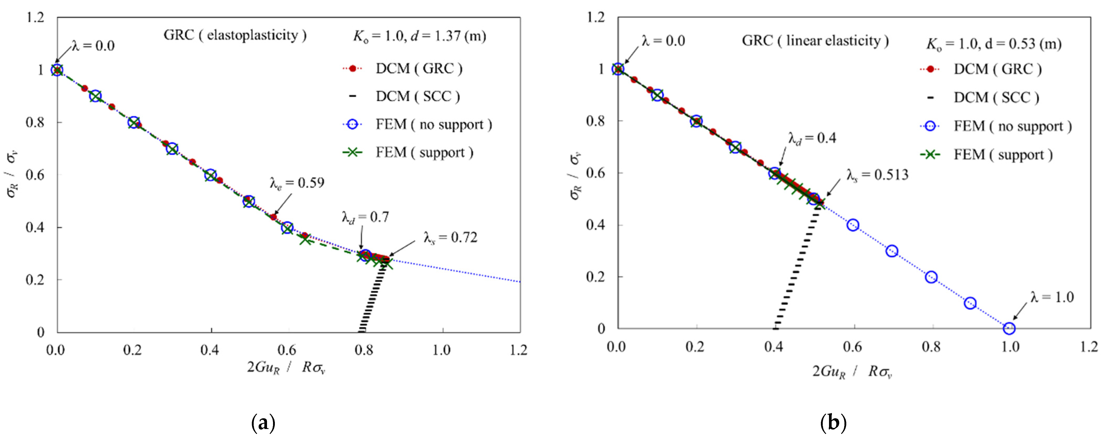
4.1. Validation of Results Obtained by Direct Analysis (DCM) and Inverse Analysis (ICM)

In direct analysis (DCM), a fixed excavation advance distance (or unsupported span, d) is usually used to simulate the effect of progressive tunnel excavation on the stress change of surrounding rock. In this study, the shotcrete-lining support system with a short unsupported span is used to simulate the stress state of the surrounding rock in the elastic range, and a long unsupported span is used to describe the stress state in the plastic range. Moreover, the convergence difference (Δu_R) is the difference of the radial displacement between the support installation (point C) and the equilibrium state (point E).

The validity of the developed direct algorithm process for the analytical solution was examined by numerical analysis, specifically, finite element analysis (FEM). The mesh made by finite element analysis includes 1971 total nodes and 658 elements (118 T6 elements and 540 Q8 elements), using three components of calculation (ground, excavation, and lining), and the analysis boundary of the roller support is 20 times the tunnel excavation radius.

Table 1. Input data of the computation of DCM and FEM.

Rock Mass Properties				Shotcrete-Lining
Parameter	Value	Parameter	Value	Parameter	Value
γ (MPa/m)	0.027	c (MPa)	0.1	γshot (MPa/m)	0.025
Em (MPa)	300.0	φ (°)	30.0	Eshot (GPa)	25.0
ν	0.25	ψ (°)	30.0	νshot	0.2
Ko	1.0	R (m)	5.2	tshot (m)	0.2
σv (MPa)	1.0	d (m)	0.53 *, 1.37 **	σc(shot) (MPa)	20.0

* Short unsupported span (d = 0.53 m), ** Long unsupported span (d = 1.37 m).

shows the input data of the computation used by DCM and FEM.

According to the results obtained by FEM and DCM, the stress/displacement in the equilibrium state is different in the plastic region (Figure 4a) and the elastic region (Figure 4b). One can find that there is a higher value of mobilized support pressure and a lower value of radial displacement in the elastic region, but on the contrary in the plastic region. Besides, one must be aware that the trace of support-ground interaction follows the curve of ground reaction, and therefore the interaction curve (IC) and the ground reaction curves (GRC) coincide with each other in this case, the isotropic stress fields. As the result shows, the values of convergence difference equal 2.545 (mm) and 1.407 (mm) for the short and long unsupported spans, respectively. One can observe that the long unsupported span gives a small value of the convergence difference for the same behavior of the ground. As a longer unsupported span means that more convergence occurs, so when the equilibrium point is reached, the required convergence difference becomes smaller.

Furthermore, to verify the calculation results of the ICM, the first step is to use the input data of the DCM (as shown in Table 1), which especially contains the initial value of the modulus of rock mass (E_m). In addition, the next computational step is to use an inverse algorithmic procedure to find an approximate convergent value for the E_m. The results obtained by the inverse analysis (ICM) indicate a good estimation for the modulus of rock mass (E_m), and the percentage error is 5.33% for the unsupported span (d) as shown in

Table 2. Output data obtained by ICM compared with the input data of DCM.

Analysis Results	DCM Em (MPa)	DCM d (m)	ICM Em (MPa) (Error * %)	ICM d (m) (Error * %)
Short unsupported span	300.0	0.53	300.0 (0.0%)	0.532 (0.38%)
Long unsupported span	300.0	1.37	300.0 (0.0%)	1.443 (5.33%)

* Error (%) = |(ICM − DCM)/DCM| × 100%.

.

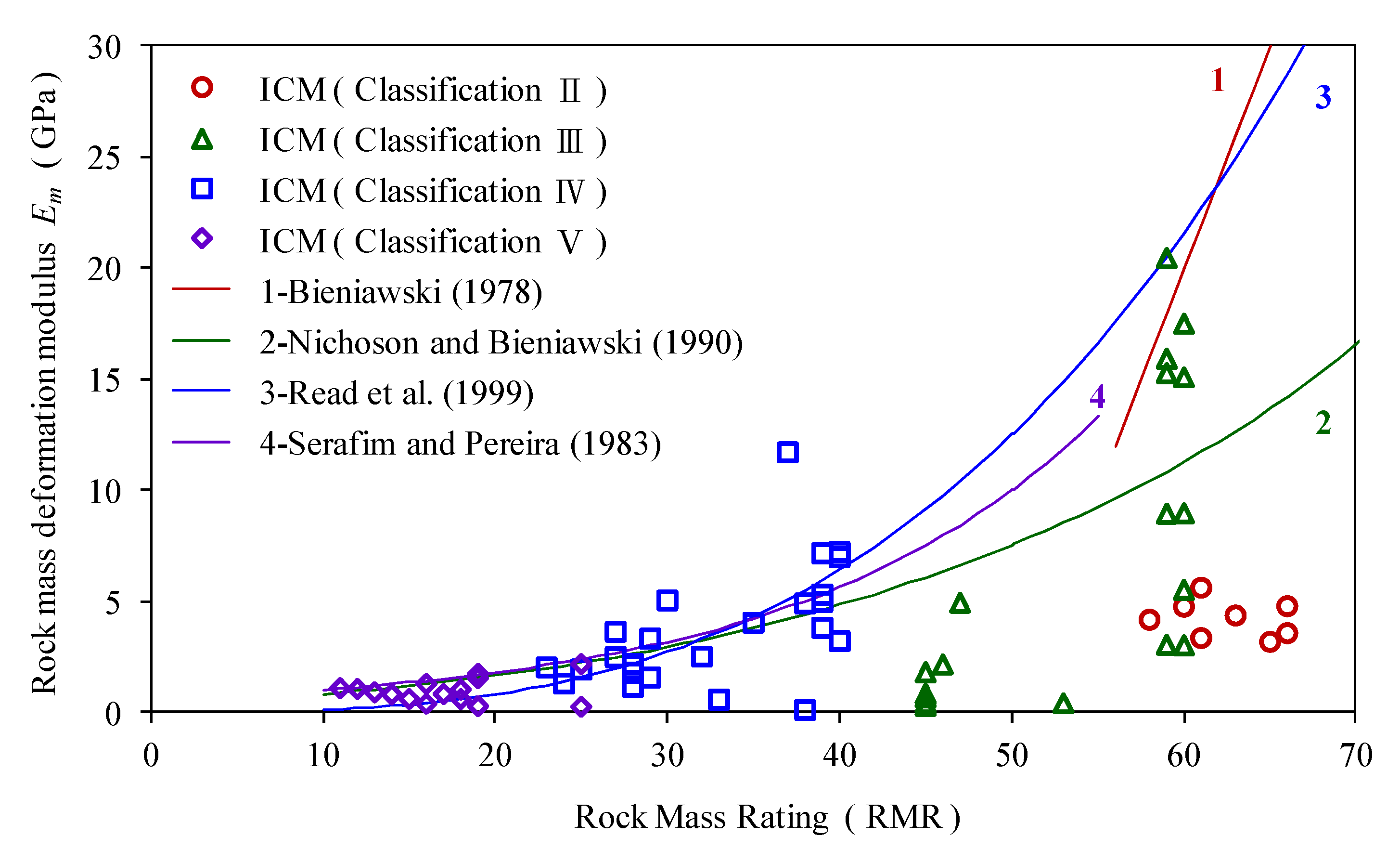
4.2. Comparison of Calculation Results between ICM and Other Studies

The case study compared with ICM includes kinds of research that are Rocksupport (2004) [20], Oreste (2009) [19], and Gschwandtner-Galler (2012) [26]. For the analysis of the ground reaction due to the tunnel excavation under the support condition, in the order of the above-listed articles, the input data of the numerical computation of ICM and listed articles are expressed in

Table 3. Input data of the numerical computation of ICM and Rocksupport (2004) [20].

Rock Mass Properties				Rock Bolt		Shotcrete-Lining
Parameter	Value	Parameter	Value	Parameter	Value	Parameter	Value
γ (MPa/m)	0.027	c (MPa)	0.15	Sc (m)	1.0	γshot (MPa/m)	0.025
Em ** (MPa)	353.0	φ (°)	25.64	Scl (m)	1.0	Eshot (GPa)	25.0
ν	0.3	ψ (°)	0.0	l (m)	6.0	νshot	0.2
Ko	1.0	R (m)	6.0	Eb (GPa)	207.0	tshot (m)	0.05
σv (MPa)	1.61	d * (m)	3.0	db (mm)	34.0	σc(shot) (MPa)	35.0

* Unsupported span, ** Modulus of the rock mass.

,

Table 4. Input data of the numerical computation of ICM and Oreste (2009) [19].

Rock Mass Properties				Support Stiffness
Parameter	Value	Parameter	Value	Parameter	Value
γ (MPa/m)	0.027	c (MPa)	0.85	ks (MPa/m)	200.0
Em ** (MPa)	8250.0	φ (°)	50.0
ν	0.25	ψ (°)	10.0
Ko	1.0	R (m)	4.0
σv (MPa)	8.1	d * (m)	0.76

* Unsupported span, ** Modulus of the rock mass.

and

Table 5. Input data of the numerical computation of ICM and Gschwandtner-Galler (2012) [26].

Rock Mass Properties				Shotcrete-Lining
Parameter	Value	Parameter	Value	Parameter	Value
γ (MPa/m)	0.027	c (MPa)	0.382	γshot (MPa/m)	0.025
Em ** (MPa)	846.0	φ (°)	27.35	Eshot (GPa)	15.0
ν	0.35	ψ (°)	27.35	νshot	0.2
Ko	1.0	R (m)	5.5	tshot (m)	0.15
σv (MPa)	5.0	d * (m)	2.0	σc(shot) (MPa)	25.0

* Unsupported span, ** Modulus of the rock mass.

.

According to the results obtained by DCM (using input data shown in Table 3) in the study of Rocksupport (2004), the values of convergence difference (Δu_R) equal 7.04 (mm) and 3.16 (mm) for the support system of rock bolt and rock bolt plus shotcrete-lining, respectively. In addition, the values of convergence difference (Δu_R) equal 2.88 (mm) and 11.43 (mm) for Oreste (2009) and Gschwandtner-Galler (2012), respectively. One can observe that the combined support system gives a small value of the convergence difference for the same behavior of the ground. In other words, in the inverse analysis (ICM), the unknown parameter, Δu_R, is the necessary input data. For the results obtained by ICM shown in

Table 6. Output data and comparison of results between ICM and other studies [19,20,26].

Other Studies Results	DCM Em (MPa)	DCM d (m)	ICM Em (MPa) (Error * %)	ICM d (m) (Error * %)
Rocksupport (2004) Bolt	353.0	3.0	353.0 (0.0%)	3.29 (8.81%)
Rocksupport (2004) Bolt + Shotcrete-lining	353.0	3.0	353.0 (0.0%)	3.13 (4.33%)
Oreste (2009)	8250.0	0.76	8250.0 (0.0%)	0.76 (0.0%)
Gschwandtner-Galler (2012)	846.0	2.0	846.0 (0.0%)	2.15 (7.5%)

* Error (%) = |(ICM − DCM)/DCM| × 100%.

, the modulus of rock mass (E_m) can be well estimated. In addition to the better simulation results of Oreste (2009), other studies have shown a percentage error range of 4.33% to 8.81% for unsupported spans (d).

As shown in Figure 5a, the values indicated by the arrows in the figure are the comparison results of the ICM calculation and the listed research values, and the remaining points are the extended calculations with various values of the convergence difference. It shows the good relationship between E_m and Δu_R by comparing with the results of the listed articles. Moreover, the function of E_m is the power function that is inversely proportional to the first power of Δu_R/R. The range of constant proportionality is from 0.02 to 0.6, as shown in Figure 5b.

For a fixed-length unsupported span, a smaller value of the tunnel convergence difference, a larger value of the modulus of rock mass, which can further indicate that the overall geomechanical behavior, is in a good state. Furthermore, for tunneling in a specific rock mass (fixed E_m value), a larger value of tunnel convergence difference (Δu_R) indicates that a shorter unsupported span is required, as shown in Figure 6a. After display via dimensionless normalization for tunnel excavation radius (R), the curve-fitting for this relationship can be interpreted by the logarithmic function shown in Figure 6b. In other words, there is a specific functional relationship between the unsupported span and the convergence difference. The unsupported span estimated by using the convergence measurement in tunnel engineering practice is presented by the inverse analysis in this paper.

As is known in logic, necessity (ICM) and sufficiency (DCM) are terms used to describe a conditional or implicational relationship between states. Therefore, this principle is verified and satisfied in this study.

5. Case Study of the Railway Tunnels

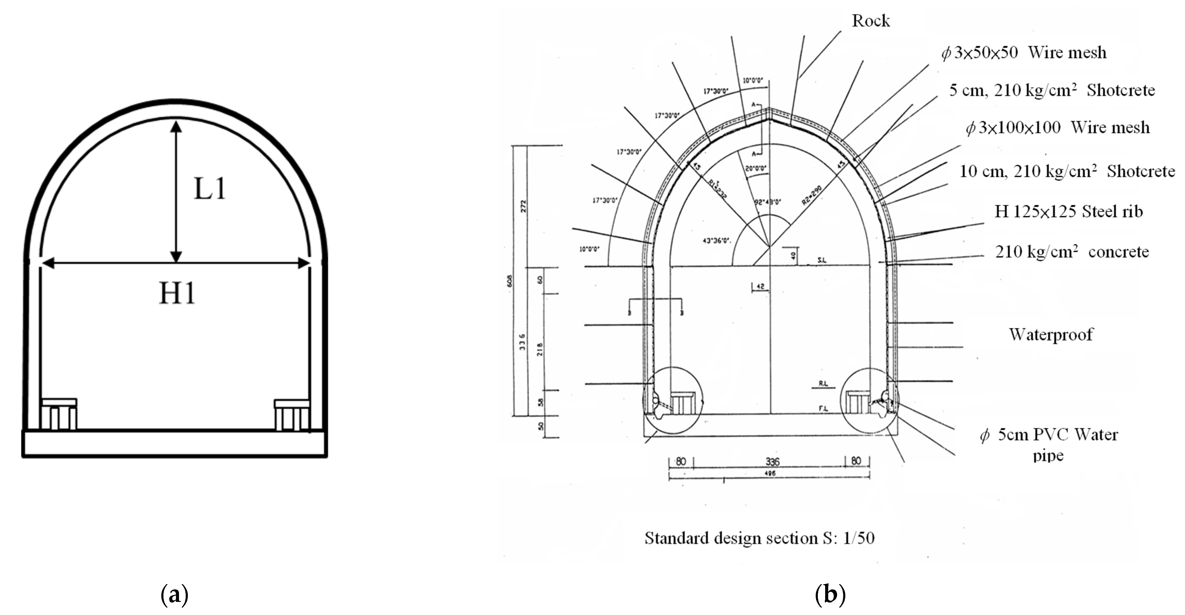
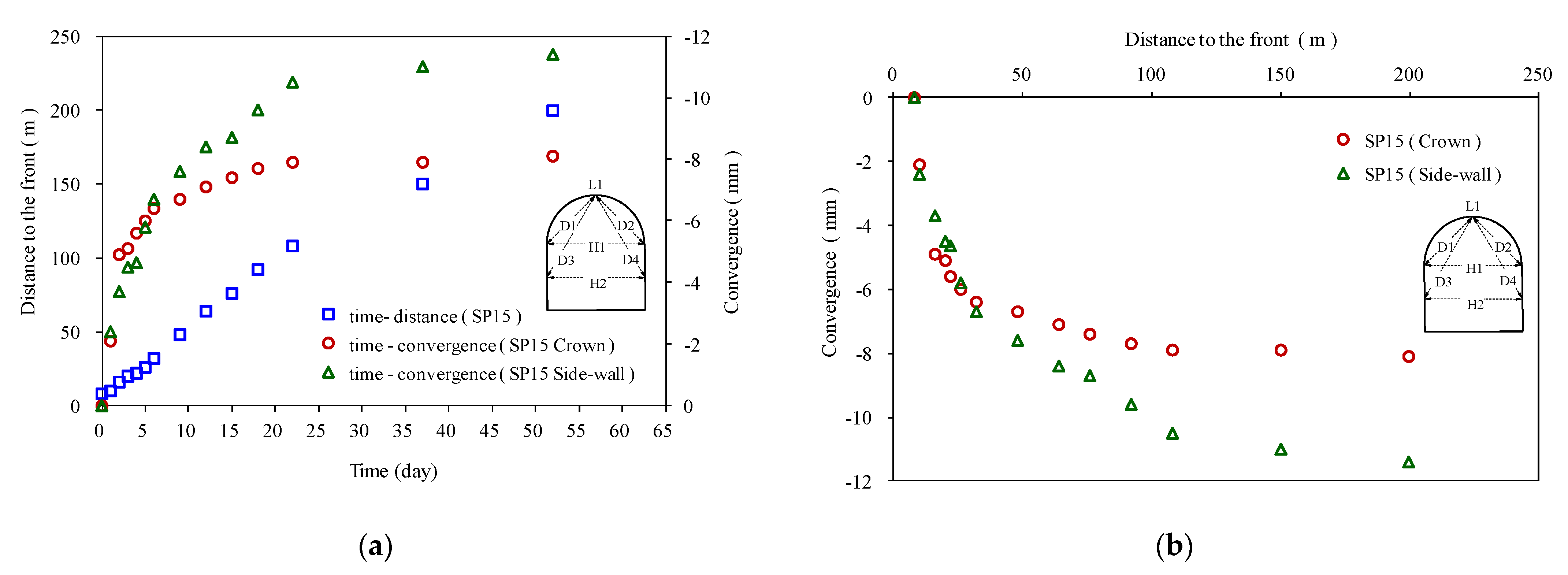
5.1. General Geology, Preliminary Data, Tunnel Design, and Monitoring Data

The two railway tunnels are located in North East Taiwan, about 15 km south of Suao city. It will serve as part of the transportation system between Suao city and Hualien city. It is an individual tunnel project and it is approximately 4460 m and 5344 m long for the New Youngchun tunnel and New Nanao tunnel, respectively. Two railway tunnels have been constructed in the highly tectonic regions and in the metamorphic rock formations which consist of the schist, slate, amphibolite, sandstone, and gneiss. The maximum heights of overburden for the New Youngchun tunnel and New Nanao tunnel are 966 m and 1013 m, respectively.

According to the rock mass classification system, the CSIR-RMR, which includes the five grades of I, II, III, IV, and V, can be utilized to categorize the properties of rock mass, design of support types, and to exhibit a length of excavation in the reconstruction project of railway tunnels. As a result, two railway tunnels pass mostly through rock mass grades III-V. The standard design section and the measurement points, L1 (top heading) and H1 (bench), of the observation section of two railway tunnels where tunnel radii are 3 m, are shown in Figure 7.

Field monitoring is essential in the observational method of tunneling. Monitoring provides valuable information, especially for inverse analysis purposes, and feedback from the surrounding ground for the safety of the work. The sequential excavation of the New Youngchun tunnel and New Nanao tunnel was designed under anticipated ground conditions and the excavation sequence varied in the two tunnels. During construction, 68 sections of observation were fully instrumented. Displacement measurements on the tunnel boundary are conducted with surveying measurements with a tape extensometer. The 68 fully instrumented sections are partially shown in

Table 7. Parameters of the observation in part of the 68 sections in two railway tunnels.

Section No.	Depth H (m)	Cohesion c (MPa)	Friction Angle φ (deg.)	Poisson’s Ratio ν	RMR *	Em ** (GPa)	Support Stiffness ks (MPa)	Convergence Difference ΔuR (mm)
SP30	403.0	0.15	20	0.33	40	5.623	1302	16.3
SP28	419.0	0.15	20	0.33	32	3.548	1302	16.3
SP21	253.0	0.25	30	0.33	60	20.0	868	7.8
SP16	301.0	0.25	30	0.33	47	8.414	868	16.3
SP15	301.0	0.25	30	0.33	52	18.0	868	8.3
YNS21	283.9	0.25	30	0.33	45	7.499	868	21.0
YNS17	238.5	0.10	15	0.31	17	1.496	1736	16.0
YNS15	246.9	0.15	20	0.33	28	2.818	1302	13.0
YNS9	82.6	0.10	15	0.31	15	1.334	1736	10.0
YSS23	258.9	0.15	20	0.33	29	2.439	1302	12.0
YSS12	111.9	0.35	40	0.31	61	22.0	434	4.0
YSS9	119.1	0.35	40	0.31	58	16.0	434	4.0
YSS8	94.3	0.25	30	0.33	45	7.499	868	4.0

* RMR: Rock mass rating, ** Estimated by using the equation of Serafim and Perira (1983) [30].

along with the corresponding estimates of the rock mass grade. In Table 7, the sections of observation including the information of the mileage, properties of rock mass, stiffness of the supports, stress conditions, and convergence measurements at the crown and side-wall are investigated in this study.

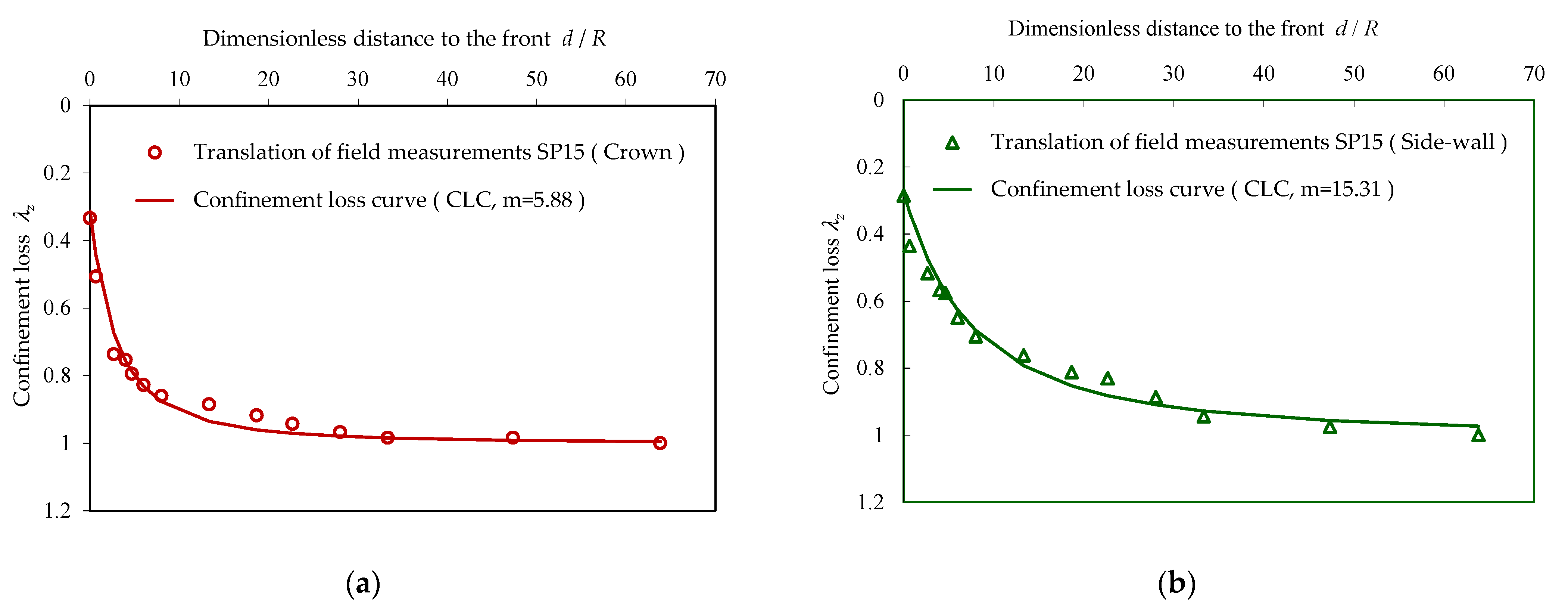
5.2. Establishment of Confinement Loss Curve (CLC)

With respect to the steps of inverse calculation in the inverse analysis, the establishment of a confinement loss curve (CLC) is the first step in the treatment of the field measurements including the time of sequential construction, the section of observation at a distance to the front and convergence. For example, the field measurements at the section of observation SP15 of the New Nanao tunnel are shown in Figure 8a. Then the illustration of the longitudinal displacement profile (LDP) is drawn with the relationship between convergence and distance to the front and shown in Figure 8b. After this, one can obtain the CLC which can be derived by the LDP with the translation of coordinates from point C to the front (the working face of the tunnel). Therefore, the confinement loss curve can be established in this step and is shown in Figure 9.

5.3. Results Obtained by the Direct Analysis (DCM)

In the following step of the analysis, the direct calculation method (DCM) is employed to find out the mobilized support pressure and the radial displacement in the equilibrium state. In this step, it is necessary to consider various parameters at different locations of the intrados of the tunnel which are the stress conditions, coefficient of regression, locations in the polar coordinates, the convergence (maximum relative displacements between point C and E) at the crown and side-wall, and the parameters for calculation which are the tunnel radius, stiffness of supports, properties of rock mass (unit weight, Poisson’s ratio, internal friction angle, and cohesion) and the unsupported span.

The parameters of the sections of observation SP15 and YNS15 for the inverse analysis are presented in Table 6. The results obtained by the direct calculation method (DCM) for the section of observation SP15 and YNS15 are shown in Figure 10. It presents the interaction behavior of support-ground between DCM and FEM for the section of observation SP15 of the New Nanao tunnel and YNS15 of the New Youngchun tunnel. One can observe that, firstly, the agreement between the finite element results and the proposed closed-form solutions in the direct analysis (DCM) was found to be excellent in elastic and elastic-perfectly plastic media; and secondly, the maximum relative radial displacements at crown and side-wall achieved by the DCM approximately coincide with the field measurements at SP15 and YNS15.

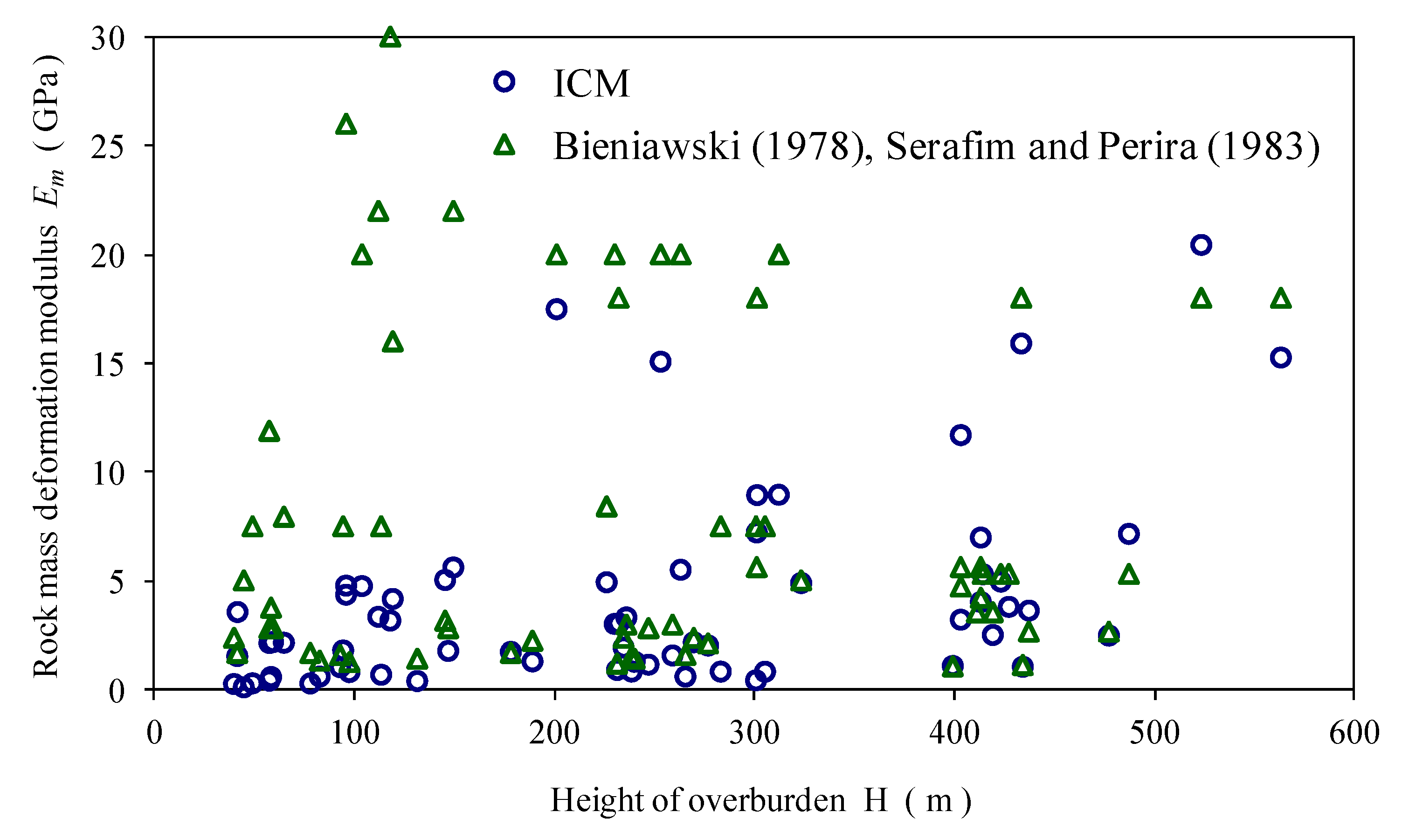
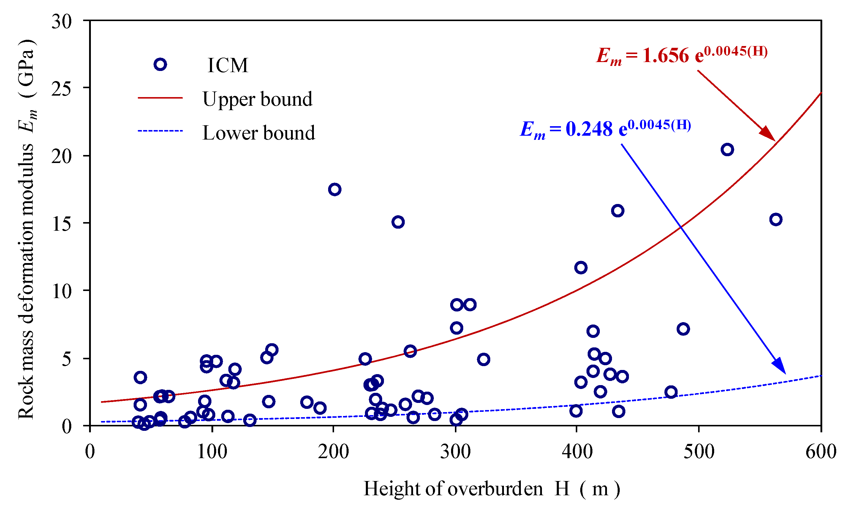
5.4. Results Obtained by the Inverse Analysis (ICM)

After all inverse calculations of the 68 sections of observation, it is evident that the 68 values of modulus of rock mass (E_m) can be therefore predicted by the ICM and represented in different categories with the rock mass grade. According to the classification system of rock mass rating (RMR), the relationships between E_m and RMR are shown in Figure 11 with the comparison of the empirical models postulated by Bieniawski (1978) [31], Serafim and Perira (1983) [30], Nicholson and Bieniawski (1990) [32], and Read et al. (1999) [33].

As a result, the classification system proposed by the reports of the reconstruction project of railway tunnels, the modulus of rock mass (E_m) distributed from the classification II to V, and the mostly obtained results are in the rock mass grade IV and V. In addition, another presentation with the category of railway tunnel can be investigated in Figure 12. It can be seen that the values of E_m of the New Youngchun tunnel are smaller than those of the New Nanao tunnel, which are more in line with the empirical models. Through this study, the agreement between the ICM and empirical models was found to be excellent from 10 to 40 in the RMR system.

From the point of view of the relationship between the modulus of rock mass (E_m) and height of overburden (H), Figure 13 shows that there is no precise relation with the height of overburden, but one can find that the values of E_m approximate a range from 0.5 GPa to 5 GPa that are the values estimated and employed to the tunnel design in these regions. Besides, if it is necessary to have the equations of predicting the relationship between the E_m and H, then the upper bound and lower bound are proposed by using the regression analysis and expressed by the exponential functions shown in Figure 14. Finally, as excellent obtained results, the modulus of rock mass surrounding a tunnel can be directly predicted by the inverse analysis (ICM).

Regarding the discussion of the results of this study, the assumption adopted by the current ICM theory is to assume that the support confining curve (SCC) is an elastic mode, but this curve in actual engineering is a nonlinear state (for example, the effect of shotcrete on time-dependence) which needs to be studied further. In addition, for the case study of two railway tunnels, the assumption of an isotropic stress field is used to inversely calculate the modulus of the rock mass. However, in order to more realistically reflect the stress conditions of the overburden above the tunnel, the influence of the anisotropic stress field must be considered so as to make the prediction of the rock modulus of the tunnel excavation more complete and referential.

6. Conclusions

Through a series of analysis processes, numerical verification, and comparison, this research can draw the following conclusions:

(1) The objective for estimation of the modulus of rock mass and the unsupported span was achieved by the inverse analysis which was particularly proposed in this paper, and the agreement between this algorithm procedure and empirical models was found to be excellent in the RMR system by the case studies of the reconstruction project of railway tunnels in Taiwan. (2) For the results obtained by ICM in a real case study of two railway tunnels under a fixed unsupported span, a large value of the convergence difference indicates the small modulus of rock mass predicted and also shows that the short unsupported span should be applied. (3) This study adopts the incremental concept of the convergence-confinement method and proposes an inverse analysis model to estimate the unknown parameters of the surrounding rock for tunnel excavation. (4) The ICM is proposed to deal with the estimation of the modulus of rock mass and the unsupported span through a special parameter that is the convergence difference between two points (the difference of the radial displacement at the support installation and the equilibrium states). (5) The theoretical analysis of the interaction of support-ground due to the excavation of a circular tunnel in isotropic stress fields is investigated by using direct analysis (DCM). (6) The confinement loss defining the situation of tunnel advancing excavation is classified by three cases (Case I, II, and III), and proposed to distinguish whether the stress state is in the elastic or the plastic regions. (7) We propose the use of the method of simultaneous equations in the elastic region and using Newton’s recursive method for finding roots in the plastic region in order to solve the solutions of support-ground interaction in the equilibrium state.

References

1. Finno, R.J.; Calvello, M. Supported excavations: The observational method and inverse modeling. J. Geotech. Geoenviron. Eng. 2005, 131, 826–836. [Google Scholar] [CrossRef]
2. Mauldon, A.D.; Karasaki, K.; Martel, S.; Long, J.C.S.; Landsfeld, M.; Mensch, A.; Vomvoris, S. An inverse technique for developing models for fluid flow in fracture systems using simulated annealing. Water Resour. Res. 1993, 29, 3775–3789. [Google Scholar] [CrossRef]
3. Gioda, G.; Sakurai, S. Back analysis procedures for the interpretation of field measurements in geomechanics. Int. J. Numer. Anal. Methods Geomech. 1987, 11, 555–583. [Google Scholar] [CrossRef]
4. Oreste, P. Back-analysis techniques for the improvement of the understanding of rock in underground constructions. Tunnell. Undergr. Space Technol. 2005, 20, 7–21. [Google Scholar] [CrossRef]
5. Luo, Y.B.; Chen, J.X.; Chen, Y.; Diao, P.S.; Qiao, X. Longitudinal deformation profile of a tunnel in weak rock mass by using the back analysis method. Tunnell. Undergr. Space Technol. 2018, 71, 478–493. [Google Scholar] [CrossRef]
6. Sharifzadeh, M.; Tarifard, A.; Moridi, M.A. Time-dependent behavior of tunnel lining in weak rock mass based on displacement back analysis method. Tunnell. Undergr. Space Technol. 2013, 38, 348–356. [Google Scholar] [CrossRef]
7. Sakurai, S.; Takeuchi, K. Back analysis of measured displacements of tunnels. Rock Mech. Rock Eng. 1983, 16, 173–180. [Google Scholar] [CrossRef]
8. Sakurai, S. Lessons learned from field measurements in tunneling. Tunnell. Undergr. Space Technol. 1998, 12, 453–460. [Google Scholar] [CrossRef]
9. Sakurai, S.; Akutagawa, S.; Takeuchi, K.; Shinji, M.; Shimizu, N. Back analysis for tunnel engineering as a modern observational method. Tunnell. Undergr. Space Technol. 2003, 18, 185–196. [Google Scholar] [CrossRef]
10. Gao, W.; Ge, M. Back analysis of rock mass parameters and initial stress for the Longtan tunnel in China. Eng. Comput. 2016, 32, 497–515. [Google Scholar] [CrossRef]
11. Li, F.; Wang, J.A.; Brigham, J.C. Inverse calculation of in situ stress in rock mass using the surrogate-model accelerated random search algorithm. Comput. Geotech. 2014, 61, 24–32. [Google Scholar] [CrossRef]
12. Zhang, L.Q.; Yue, Z.Q.; Yang, Z.F.; Qi, J.X.; Liu, F.C. A displacement-based back-analysis method for rock mass modulus and horizontal in situ stress in tunneling–Illustrated with a case study. Tunnell. Undergr. Space Technol. 2006, 21, 636–649. [Google Scholar] [CrossRef]
13. Diao, H.; Liu, H.; Sun, B. On a local geometric property of the generalized elastic transmission eigenfunctions and application. Inverse Probl. 2021, 37, 105015. [Google Scholar] [CrossRef]
14. Fang, X.; Deng, Y. Uniqueness on recovery of piecewise constant conductivity and inner core with one measurement. Inverse Probl. Imaging 2018, 12, 733–743. [Google Scholar] [CrossRef] [Green Version]
15. Deng, Y.; Li, H.; Liu, H. Spectral Properties of Neumann-Poincaré Operator and Anomalous Localized Resonance in Elasticity Beyond Quasi-Static Limit. J. Elast. 2020, 140, 213–242. [Google Scholar] [CrossRef] [Green Version]
16. Panet, M. Le Calcul des Tunnels par la Méthode de Convergence-Confinement; Presses de l’Ecole Nationale des Ponts et Chaussées: Paris, France, 1995. [Google Scholar]
17. Carranza-Torres, C.; Fairhurst, C. Application of the convergence-confinement method of tunnel design to rock masses that satisfy the Hoek–Brown failure criterion. Tunnell. Undergr. Space Technol. 2000, 15, 187–213. [Google Scholar] [CrossRef]
18. Oreste, P. Analysis of structural interaction in tunnels using the convergence-confinement approach. Tunnell. Undergr. Space Technol. 2003, 18, 347–363. [Google Scholar] [CrossRef]
19. Oreste, P. The convergence–confinement method: Roles and limits in modern geomechanical tunnel design. Am. J. Appl. Sci. 2009, 6, 757–771. [Google Scholar] [CrossRef] [Green Version]
20. Rocksupport. Rock Support Interaction and Deformation Analysis for Tunnels in Weak Rock; Tutorial Manual of Rocscience Inc.: Toronto, ON, Canada, 2004; pp. 1–76. [Google Scholar]
21. Lee, Y.L. Explicit analysis for the ground-support interaction of circular tunnel excavation in anisotropic stress fields. J. Chin. Inst. Eng. 2020, 43, 13–26. [Google Scholar] [CrossRef]
22. Lee, Y.L. Explicit procedure and analytical solution for the ground reaction due to advance excavation of a circular tunnel in an anisotropic stress field. Geotech. Geol. Eng. 2018, 36, 3281–3309. [Google Scholar] [CrossRef]
23. Brown, E.T.; Bray, J.W.; Ladanyi, B.; Hoek, E. Ground response curves for rock tunnels. J. Geotech. Eng. ASCE 1983, 109, 15–39. [Google Scholar] [CrossRef]
24. Carranza-Torres, C.; Engen, M. The support characteristic curve for blocked steel sets in the convergence-confinement method of tunnel support design. Tunnell. Undergr. Space Technol. 2017, 69, 233–244. [Google Scholar] [CrossRef]
25. De La Fuente, M.; Taherzadeh, R.; Sulem, J.; Nguyen, X.S.; Subrin, D. Applicability of the convergence-confinement method to full-face excavation of circular tunnels with stiff support system. Rock Mech. Rock Eng. 2019, 52, 2361–2376. [Google Scholar] [CrossRef]
26. Gschwandtner, G.G.; Galler, R. Input to the application of the convergence confinement method with time-dependent material behavior of the support. Tunnell. Undergr. Space Technol. 2012, 27, 13–22. [Google Scholar] [CrossRef]
27. Lee, Y.L. Establishment of the confinement loss curve using the tunnel convergence data. J. Chin. Inst. Eng. 2020, 43, 613–627. [Google Scholar] [CrossRef]
28. Mousivand, M.; Maleki, M.; Nekooei, M.; Msnsoori, M.R. Application of Convergence-Confinement method in analysis of shallow non-circular tunnels. Geotech. Geol. Eng. 2017, 35, 1185–1198. [Google Scholar] [CrossRef]
29. Vlachopoulos, N.; Diederichs, M. Improvement to the convergence-confinement method: Inclusion of support installation proximity and stiffness. Rock Mech. Rock Eng. 2018, 51, 1495–1519. [Google Scholar] [CrossRef]
30. Serafim, J.L.; Pereira, J.P. Consideration of the geomechanical classification of Bieniawski. In Proceedings of the International symposium on engineering geology and underground construction, Lisbon, Portugal, 12–15 September 1983; Volume 1, pp. 1133–1144. [Google Scholar]
31. Bieniawski, Z.T. Determining rock mass deformability—Experience from case histories. Int. J. Rock Mech. Min. Sci. 1978, 15, 237–247. [Google Scholar] [CrossRef]
32. Nicholson, G.A.; Bieniawski, Z.T. A Nonlinear deformation modulus based on rock mass classification. Int. J. Min. Geol. Eng. 1990, 8, 181–202. [Google Scholar] [CrossRef]
33. Read, S.A.L.; Perrin, N.D.; Richards, L.R. Applicability of the Hoek-Brown failure criterion to New Zealand Greywacke rocks. In Proceedings of the 9th ISRM Congress, Paris, France, 25–28 August 1999. [Google Scholar]
Figure 1. Graphical concept of the support-ground interaction in the analysis of CCM.
Mathematics 10 01223 g001
Figure 2. Explicit algorithm process of DCM and ICM in the analysis of CCM in tunneling.
Mathematics 10 01223 g002
Figure 3. Computational flowchart of the ICM.
Mathematics 10 01223 g003
Figure 4. Comparison of results obtained between DCM and FEM. (a) in the plastic region (long unsupported span), and (b) in the elastic region (short unsupported span).
Mathematics 10 01223 g004
Figure 5. Estimation of the modulus of rock mass (Em) from the difference of the radial displacement between point C and point E in the analysis (ICM). (a) The comparison with the original data, and (b) the description of the regression curve.
Mathematics 10 01223 g005
Figure 6. Estimation of the unsupported span (d) from the difference of the radial displacement between point C and point E in the inverse analysis (ICM). (a) The comparison with the original data, and (b) the description of the regression curve.
Mathematics 10 01223 g006
Figure 7. (a) Measurement points L1 and H1, and (b) standard design section of the observation section at tunnel face proximity of the New Youngchun and the New Nanao railway tunnels.
Mathematics 10 01223 g007
Figure 8. Filed measurements at the section of observation SP15 of the New Nanao tunnel (a) the information of time (day) of sequential construction, convergence (mm), and distance to the front (m), (b) relationship between convergence and distance to the front.
Mathematics 10 01223 g008
Figure 9. Relationship between confinement loss and dimensionless distance to the front at the section of observation SP15 of the New Nanao tunnel (a) at crown, (b) at side-wall.
Mathematics 10 01223 g009
Figure 10. Comparison of the interaction behavior of support-ground between DCM and FEM at the section of observation (a) SP15 of the New Nanao tunnel, and (b) YNS15 of the New Youngchun tunnel.
Mathematics 10 01223 g010
Figure 11. Correlation between the modulus of rock mass predicted by the inverse analysis (ICM) and the rock mass rating (RMR) of the presentation of the two railway tunnels.
Mathematics 10 01223 g011
Figure 12. Correlation between the modulus of rock mass predicted by the inverse analysis (ICM) and the rock mass rating (RMR) of the presentation of the two railway tunnels.
Mathematics 10 01223 g012
Figure 13. Comparison of the modulus of rock mass between inverse analysis (ICM) and RMR system (from Bieniawski, 1978; Serafim and Perira, 1983) with the height of overburden.
Mathematics 10 01223 g013
Figure 14. Correlation between modulus of the rock mass predicted by the inverse analysis (ICM) and height of overburden.
Mathematics 10 01223 g014