Unsupervised Fault Diagnosis of Sucker Rod Pump Using Domain Adaptation with Generated Motor Power Curves

Abstract

The poor real-time performance and high maintenance costs of the dynamometer card (DC) sensors have been significant obstacles to the timely fault diagnosis in the sucker rod pumping system (SRPS). In contrast to the DCs, the motor power curves (MPCs), which are accessible easily and highly associated with the entire system, have been attempted to predict the working conditions of the SRPS in recent years. However, the lack of labeled MPCs limits the successful applications in the industrial scenario. Thereby, this paper presents an unsupervised fault diagnosis methodology to leverage the generated MPCs of different working conditions to diagnose the actual unlabeled MPCs. Firstly, the MPCs of six working conditions are generated with an integrated dynamics mathematical model. Secondly, a framework named mechanism-assisted domain adaptation network (MADAN) is proposed to minimize the distribution discrepancy between the generated and actual MPCs. Specifically, benefiting from introducing the mechanism analysis to label the collected MPCs preliminarily, a conditional distribution discrepancy metric is defined to guarantee a more accurate distribution matching with respect to different working conditions. Eventually, validation experiments are performed to evaluate the mathematical model and the diagnosis method with a set of actual MPCs collected by a self-developed device. The experimental result demonstrates that the proposed method offers a promising approach for the unsupervised diagnosis of the SRPS.

1. Introduction

The sucker rod pump system (SRPS) plays an indispensable role in the field of oil exploitation [1]. Due to the long-time operations and harsh working environment, some faults will inevitably occur, resulting in economic loss and energy consumption [2]. With the rapid development of machine learning, many data-driven fault diagnosis methods have been utilized to guarantee manufacturing security and improve production efficiency in the SRPS [3,4]. However, the most traditional and commonly used diagnostic methods universally depend on the dynamometer card (DC), which is measured by the load sensor installed on the “horse head”. These DC-based methods inevitably suffer from the high maintenance cost and low detection frequency, resulting in poor ability in the real-time diagnosis of the SRPS.

Owing to power’s advantages of accessibility and high correlation with the SRPS, the motor power-based diagnosis methods have received ever-increasing attention [5]. Ref. [6] distilled seven features from the motor power curves (MPCs) and utilized improved hidden conditional random fields to diagnose different working conditions. An MPC-based broad learning method was proposed in [7].

Even though conspicuous achievements have been achieved, these methodologies lack applicability due to their reliance on the massive labeled data, which is invalid in the real industrial scenarios [8]. Some researchers tried to tackle this problem by implementing a transformation between the MPC and the DC to facilitate the diagnosis based on the MPCs. In [9], the MPCs were labeled by transforming into DCs with a mechanism model considering many crucial factors. However, the inversed DCs were not closed because the torque factor was zero at the dead points, resulting in huge discrepancies between the actual and inversed DCs. Nowadays, new research transformed the DC to MPC to alleviate the discrepancies at the dead points in [10]. However, the complete DC dataset is still a problematic prerequisite for some wells with incomplete data.

In order to reduce the dependence on the labeled dataset, this paper tries to propose a model-based method to generate the MPCs. Although many scholars have been committed to the process modeling of the SRPS, their purpose is to obtain the polished load without correlating the uphole portion to simulate the MPC [11,12,13]. In this respect, this paper is dedicated to establishing an integrated dynamics mathematical model involving the motor, the four-bar linkage, the sucker rod, and the pump to generate the MPCs at normal and five kinds of faulty scenarios.

Even though the labeled MPCs can be obtained from the model-based method, the traditional intelligent diagnosis strategies trained with such samples possibly fail in classifying actual MPCs. The distribution discrepancy that arises from unavoidable assumptions and simplifications in the model limits the successful applications of these strategies. Domain adaptation (DA), which is a popular branch of transfer learning, has advantages in solving the problem of inconsistent feature distribution [14,15,16,17]. Traditional DA employs the Maximum Mean Discrepancy (MMD) term as the discrepancy penalty to extract the domain-invariant features [18,19,20]. Inspired by the idea of the generative adversarial network, the domain discriminator was explored to align the distributions in an adversarial manner [21]. Ref. [22] leveraged a one-dimensional convolutional neural network (1-D CNN) to bridge the distribution discrepancy by maximizing the discriminator loss and minimizing the classifier loss. In [23], Wasserstein distance replaced the traditional discriminator to minimize the distribution discrepancy. A strong–weak learning framework was proposed to solve the imbalanced data and mismatched domain simultaneously based on the domain adversarial training in [24]. In [25], discriminator and MMD were exploited together to enhance feature representation. The discriminator network was extended to partial domain adaptation in [26,27].

The aforementioned discriminator and MMD are dedicated to aligning the marginal probability distribution. Specifically, inspired by [28], the conditional probability distribution is also increasingly integrated into the domain adversarial training in recent years. In [29], the adversarial training was utilized to realize marginal fusion, and a variance matrix was defined to achieve conditional alignments. The joint distribution supplanted the marginal distribution for conditional distribution alignments in [30]. In [31], a pre-training network was designed for pseudo-label learning and MMD was applied to align the conditional distribution. Ref. [32] utilized the adversarial network and the joint adaptation network to alleviate the distribution discrepancy of the label and feature spaces.

Although conditional distribution alignment has made some progress to the DA, little attention has been paid to the pseudo-label learning of the target domain. The common pseudo-label methodologies rely on the traditional clustering algorithm, source domain classifier, and the pre-trained network with source domain data. Limited by the inaccuracy of the initial phase of the neural network and the huge distribution gap between the target and source domains, these algorithms will assign extensive inaccurate pseudo-labels to interfere with the domain alignment. Therefore, in order to achieve more accurate pseudo-labels to narrow down the distribution discrepancy, a novel method named mechanism-assisted domain adaptation network (MADAN) is proposed. In the MADAN, the mechanical properties of the MPCs under different working conditions are adopted for pseudo-label learning along with the label classifier. Particularly, the classifier iterates continuously with training to alleviate conditional distribution discrepancy through a well-defined MMD term. The marginal distribution alignment is implemented with the help of the adversarial domain adaptation, and 1-D CNN constructs the feature generator network to extract the features of the time-series signal.

The main contributions of this paper can be summarized as follows:

1. An integrated dynamics mathematical model is established to generate the MPCs at normal and five kinds of faulty scenarios. The model calculates “four-bar” linkage movement, sucker rod vibration, the pump chamber pressure, and the liquid flow rate. The adjustment strategies of the model and relevant parameters under different working conditions are also presented.

2. A novel DA method named MADAN is proposed to exploit the knowledge learned from the generated MPCs to facilitate diagnosing the MPCs collected in practical scenarios. The mechanism-assisted pseudo-label learning is constructed to realize better conditional distribution alignment of the collected and generated MPCs under different working conditions. Furthermore, the domain classifier is designed for the marginal distribution alignment of the collected and generated MPCs.

3. Experiments demonstrate the superiority of the proposed fault diagnosis methodology with the MPCs collected by self-developed portable devices in the practical application scenario. The model’s validity is verified by analyzing crucial downhole parameters and comparing the generated and actual MPCs. Furthermore, we experimentally show that MADAN outperforms five other state-of-the-art methods in terms of diagnostic accuracy and distribution alignment.

The rest of this article is organized as follows. The integrated dynamics mathematical model to generate the MPCs under various working conditions is surveyed in Section 2. Section 3 describes the proposed MADAN method. Section 4 shows the effectiveness of the proposed method through experimental verification. Finally, Section 5 concludes this article.

2. Generation of the Motor Power Curves

Driven by the motor, the pump connected with a series of transmissions is in a reciprocating up-and-down motion to pull the oil from the down-hole to the ground in the SRPS. As the energy for the whole system, the MPCs involve information about the SRPS working properties. Homoplastically, the MPCs of the well can be obtained by the inversion of the individual components simulation. To generate supplementary power waveforms of different working states for fault diagnosis, a detailed and integrated discussion of the mathematical model for the SRPS is presented in this section.

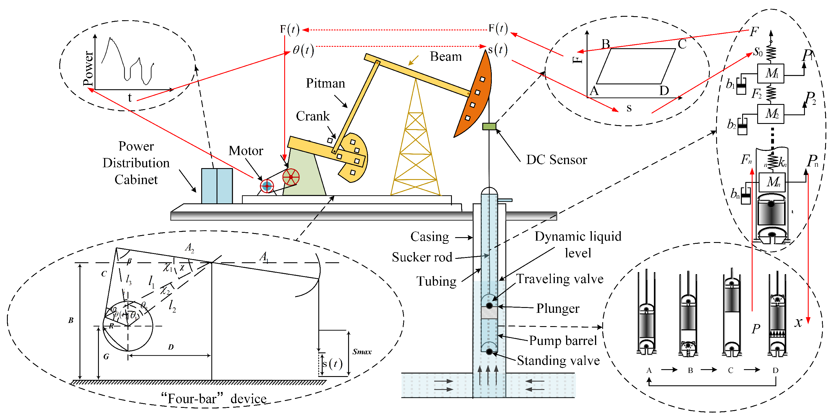
2.1. Mathematical Model of the Sucker Rod Pumping System

Figure 1 indicates a typical structure of the SRPS.

Aiming at the MPCs composed by the power vs. time, the mathematical model follows the order as the red arrows in Figure 1 as time → crank angle → polished rod motion ⇆ plunger motion ⇄ pump pressure ⇆ polished rod load → crank torque → power. The prediction of SRPS behavior involves calculating “four-bar” linkage movement, sucker rod vibration, down-hole pump simulation of the pump, etc. Of these items, the operation of the down-hole pump, the polished rod motion, and the vibrations of the rod string are of the most difficulty but primary importance. In this subsection, the establishment of the mathematical model centers on the difficulties mentioned.

2.1.1. Polished Rod Motion Simulation

As the crank angular velocity approaches constant speed in practice, the crank angle $\theta$ vs. time is given by

$$\theta \left(t\right)=\omega t=\frac{2\pi nt}{60}.$$

(1)

From trigonometrical considerations, the calculation for the displacement of the polished rod $s\left(t\right)$ is listed as follows:

$$\left\{\begin{array}{cc}\hfill s\left(t\right)& =s_{max}\frac{{\chi }_{max}-\chi }{{\chi }_{max}-{\chi }_{min}},\hfill \\ \hfill {\chi }_1& =arcsin\frac{Csin\beta }{l_1},\hfill \\ \hfill {\chi }_2& =arcsin\frac{Rsin({\theta }_1+\theta \left(t\right))}{l_1},\hfill \\ \hfill \beta & =arccos\frac{A_2^2+C^2-l_2^2-R^2+2l_{2}Rcos({\theta }_1+\theta \left(t\right))}{2A_{2}C},\hfill \\ \hfill l_1& =\sqrt{l_2^2+R^2-2l_{2}Rcos({\theta }_1+\theta \left(t\right))},\hfill \\ \hfill {\theta }_1& =arctan\frac{D}{B-G},\hfill \\ \hfill {\chi }_{max}& =arccos\frac{l_2^2+A_2^2-{(C+R)}^2}{2l_2{A}_2},\hfill \\ \hfill {\chi }_{min}& =arccos\frac{l_2^2+A_2^2-{(C-R)}^2}{2l_2{A}_2}.\hfill \end{array}\right.$$

(2)

The polished rod load is obtained as the summation torque acting on the polished rod of the crank torque, the counterbalance torque arising from the balanced weight and the net weight of the crankshaft, and counterbalance torque. The crank torque is derived backward by the relation

$$F_c=\overline{TF}(F-W_{ub}){\eta }_b^{\mu }-(W_{ck}{R}_{ck}+W_{cb}R)sin\theta \left(t\right),$$

(3)

where $\mu =1$ when $\overline{TF}<0$, and $\mu =-1$ when $\overline{TF}\geqq 0$. The torque factor as obtained from mechanics is given by

$$\overline{TF}=\frac{A_{1}R}{A_2}\frac{sin\beta }{sin\phi }.$$

(4)

2.1.2. Rod String Simulation

Considering the rod string is up to thousands of meters long, the elastic deformation and vibration should not be neglected during the reciprocating up-and-down motion. Simulation of the rod string involves the calculation of a boundary problem. The boundary upon the ground is regarded as a compulsive movement, which is determined by the motion of the polish rod. The boundary of the down-hole is decided by the pump pressure acting at the plunger and the elastic force of the rod string. Benefiting from the rod string acting as a spring-mass-damping system with multiple degrees of freedom, the rod string is divided into individual parts connected by an equivalent spring, as illustrated in Figure 1.

Combined with buoyancy, gravity, frictional damping of the rod, and tubing, the dynamic analysis of the rod string can be deduced as

$$\left\{\begin{array}{c}F=k_1(P_0-P_1-l_1),\\ M_1\ddot{P_1}+b_1\dot{P_1}+k_2(P_1-P_2-l_2)+M_{1}g-{\rho }_{o}g(P_0-P_1)S_r\\ +f_r(P_0-P_1)C_l{\sigma }_v=k_1(P_0-P_1-l_1),\\ M_2\ddot{P_2}+b_2\dot{P_2}+k_3(P_2-P_3-l_3)+M_{2}g-{\rho }_{o}g(P_1-P_2)S_r\\ +f_r(P_1-P_2)C_l{\sigma }_v=k_2(P_1-P_2-l_2),\\ ⋮\\ M_{n-1}{\ddot{P}}_{n-1}+b_{n-1}{\dot{P}}_{n-1}+k_n(P_{n-1}-P_n-l_n)+M_{n-1}g-{\rho }_{o}g(P_{n-2}\\ -P_{n-1})S_r+f_r(P_{n-2}-P_{n-1})C_l{\sigma }_v=k_{n-1}(P_{n-2}-P_{n-1}-l_{n-1}),\\ M_n{\ddot{P}}_n+b_n{\dot{P}}_n-k_n(P_{n-1}-P_n-l_n)+M_{n}g-{\rho }_{o}g(P_{n-1}-P_n)S_r\\ +f_r(P_{n-1}-P_{n-2})C_{l}t{\sigma }_v=-F_n,\end{array}\right.$$

(5)

where $\dot{P_i}$ and $\ddot{P_i}$ denote the first and second derivatives of $P_i$ regarding time, respectively. $C_l$ can be caculated as $C_l=\pi (d_p+d_r)$.

2.1.3. Down-Hole Pump Simulation

Equal to the force on the bottom of the rod string $F_n$, the force on the plunge can also be deduced from the down-hole pump simulation as follows:

$$F_n\left(t\right)=S_p(P_d-P_p\left(t\right))-S_r{P}_d+f_p{\dot{P}}_n.$$

(6)

It is mainly related to the pressure of the pump. Suffering from various coupled variables and sophisticated processes existing in the down-hole, the simulation of pressure remains a severe issue but is the core of the whole model. In order to get around this impasse, the basic concepts of iterative algorithms are applied in this subsection. The pressure proportional to the mass per unit volume of free gas can be deduced as follows:

$$P_p\left(t\right)=\frac{M_{fg}\left(t\right)\xi }{V_p\left(t\right)-V_w\left(t\right)-V_o\left(t\right)}.$$

(7)

The variation of gas, liquid, and oil in the pump can be calculated by flow rate. When the standing valve is closed, the flow rate is zero. When the standing valve is open, the flow rate can be calculated as

$$Q\left(t\right)=\frac{C_1{S}_s{\rho }_l}{\sqrt{{\sigma }_s}}\sqrt{\frac{P_p\left(t\right)-P_s}{{\rho }_l}}.$$

(8)

Considering a bit of gas dissolved in the oil, the solubility of the gas is calculated based on Henry’s Law. On the assumption that the water–oil–gas mass ratio of flows is constant in one stroke, the specific calculation is organized as follows:

$$\left\{\begin{array}{cc}\hfill M_{fg}\left(t\right)& =M_g\left(t\right)\frac{{\rho }_g(t-1)V_{fg}(t-1)}{{\rho }_g(t-1)V_{fg}(t-1)+{\delta }_g(t-1)M_o(t-1)},\hfill \\ \hfill M_g\left(t\right)& =M_g(t-1)+{\gamma }_{g}Q(t-1)△t,\hfill \\ \hfill M_o\left(t\right)& =V_o\left(t\right){\rho }_o=M_o(t-1)+{\gamma }_{o}Q(t-1)△t,\hfill \\ \hfill M_w\left(t\right)& =V_w\left(t\right){\rho }_w=M_w(t-1)+{\gamma }_{w}Q(t-1)△t,\hfill \\ \hfill {\rho }_g(t-1)& =\frac{P_p(t-1)M_{mol}}{C_2{T}_d},\hfill \\ \hfill {\delta }_g(t-1)& =C_h{P}_p(t-1).\hfill \end{array}\right.$$

(9)

An iterative equation for estimating the pump pressure $P_p$ is given as

$$\frac{P_p\left(t\right)}{P_p(t-1)}=\frac{M_{fg}\left(t\right)}{M_{fg}(t-1)}\frac{V_p(t-1)-V_w(t-1)-V_o(t-1)}{V_p\left(t\right)-V_w\left(t\right)-V_o\left(t\right)}.$$

(10)

2.1.4. Moter and Gearbox Simulation

Considering the energy loss in the gearbox and the motor, the crank toque vs. the motor power is simplified as

$$P_m=\frac{F_c{n}_m{\eta }_m^{\sigma }}{9540},whenP>0,\sigma =1,else\sigma =-1.$$

(11)

2.1.5. Dynamic Implementation of the Overall Model

As the order of the red arrows in Figure 1, Algorithm 1 outlines the procedure of the whole generating power method mentioned above combining the standing and traveling valve switch situations. By the proposed mathematical model, the theoretical MPC can be obtained based on the mechanical parameters of the specific oil well.

Algorithm 1: Generation of motor power waveforms.

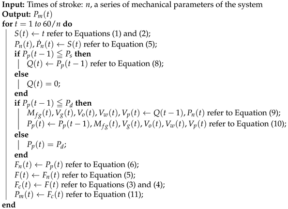
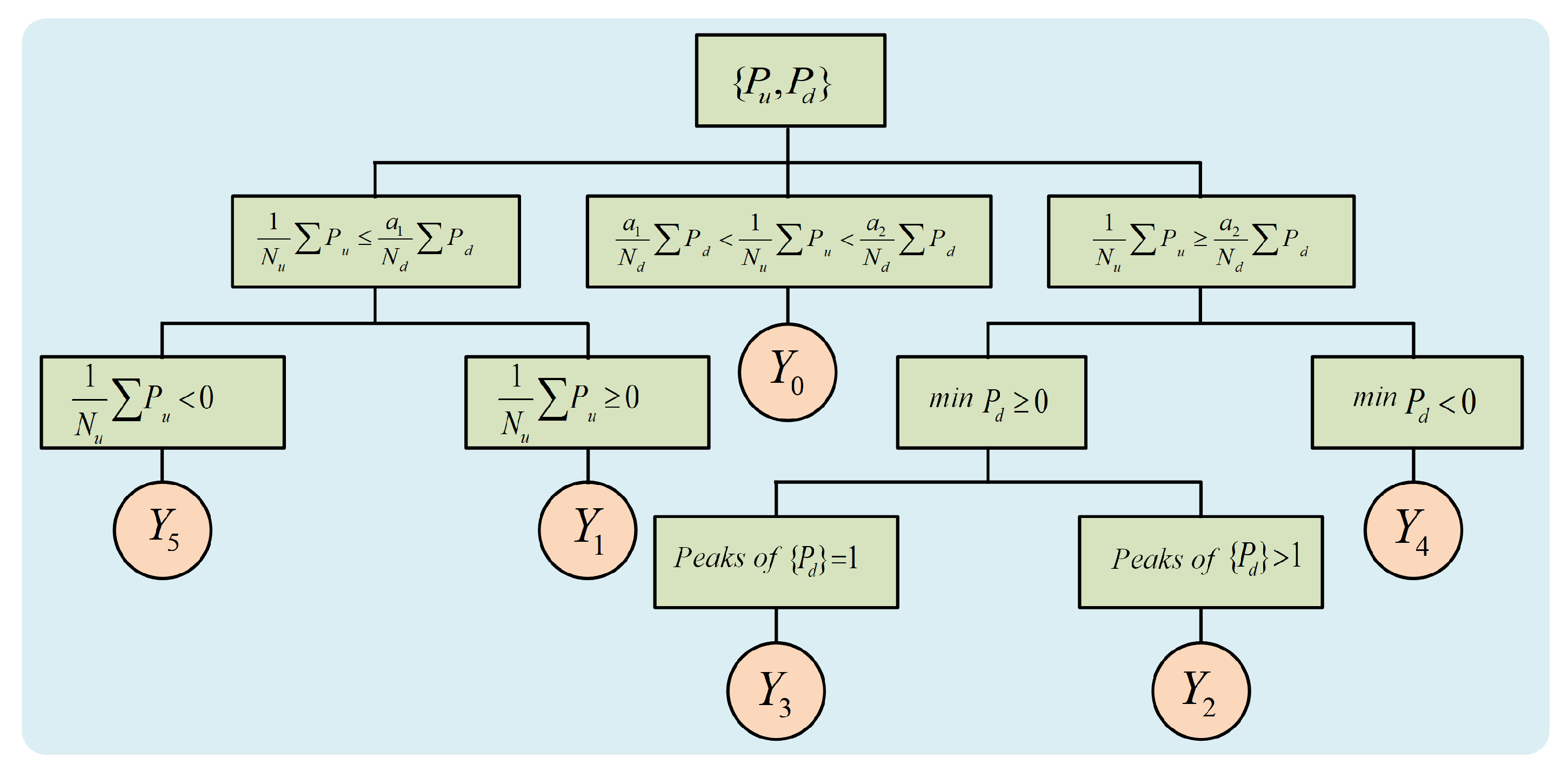
2.2. Generation for Faulty Working States

Based on the mathematical model of the SRPS, the MPCs of five faulty working states are analyzed in this subsection. The characteristics forming reasons and representation in the model will be discussed emphatically.

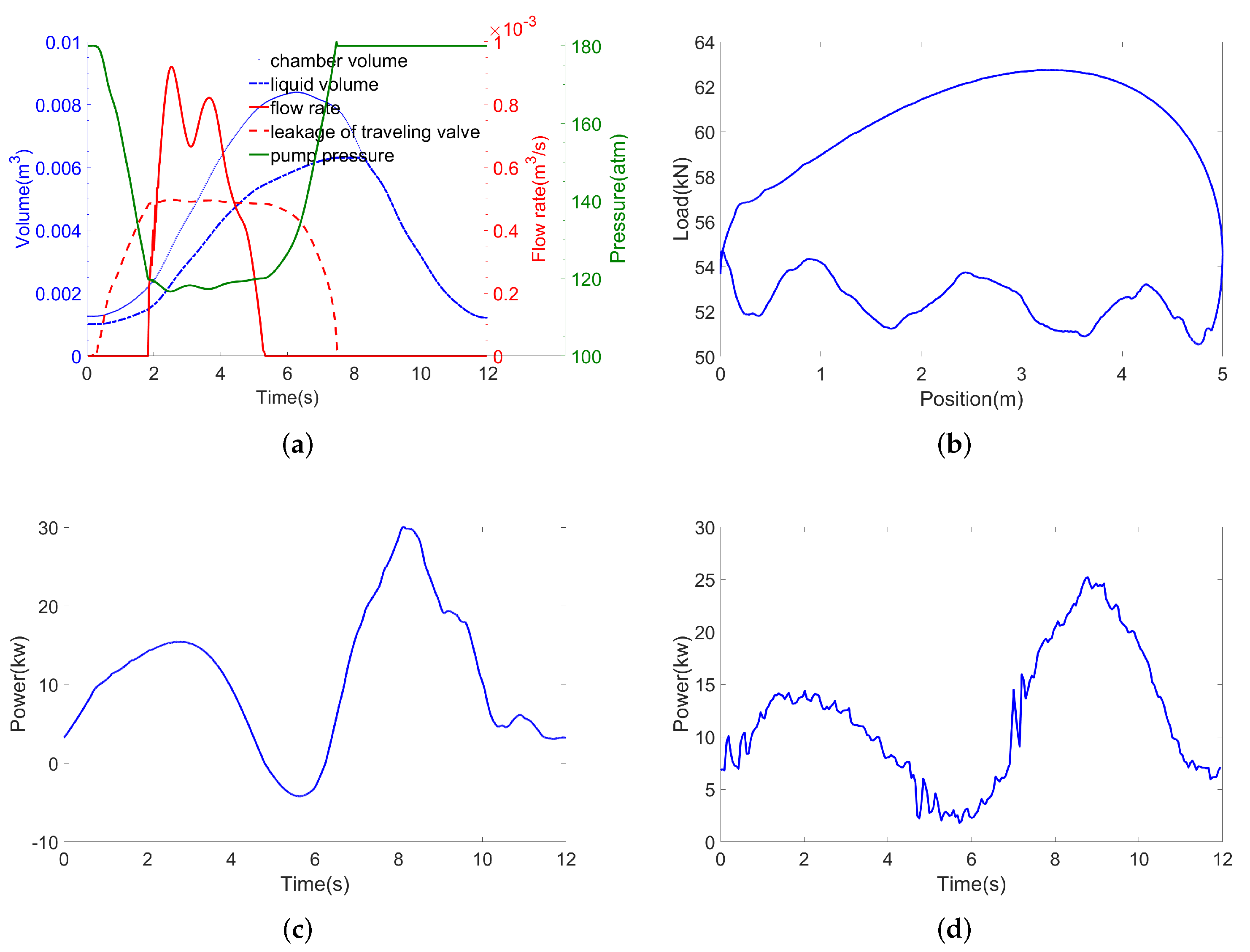
2.2.1. Traveling Valve Leakage

After repeating the switch operation numerous times, the traveling valve will wear out so that the oil in the sucker rod leaks into the chamber with the rate concerned to the $P_p\left(t\right)$. In order to simulate this state, the leaked oil is divided into static and dynamic parts. The pressure and the flow rate are the same as the normal state when the traveling valve is open. When the traveling valve is closed, the static part that is caused by the pressure discrepancy between the top and bottom of the plunger can be deduced as

$$▵Q_s\left(t\right)=\frac{{\rho }_l{C}_3{S}_{lt}}{\sqrt{{\sigma }_t}}\sqrt{\frac{P_d-P_p\left(t\right)}{{\rho }_l}}.$$

(12)

The dynamic part that is caused by the motion of the plunger can be calculated as

$$▵Q_d\left(t\right)=\pi S_{lt}{\dot{P}}_n.$$

(13)

The leaked oil can be obtained from the sum of the static part and the dynamic part.

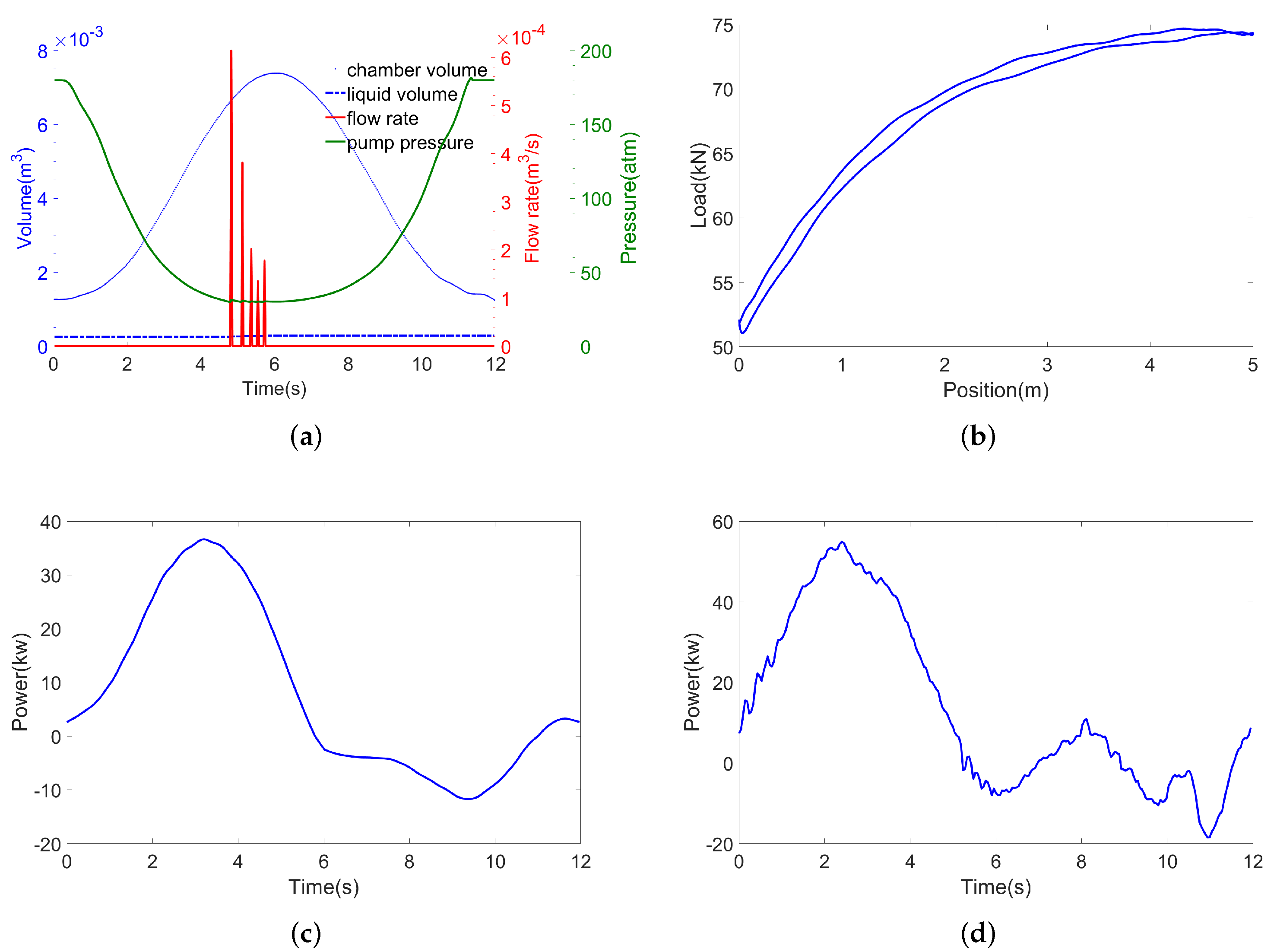
2.2.2. Insufficient Liquid Supply

After a long extraction period, the reservoir formation pressure usually decreases, resulting in insufficient fluid supply capacity. In this working state, the submergence pressure $P_s$ is less than the pressure under the normal working state. There will be less oil flowing into the pump, and the traveling valve will open in a shorter time. To simulate this working state, only the submergence pressure $P_s$ needs to be set as a smaller value.

2.2.3. Gas Affected

During the oil production process, the remaining free gas accumulates due to the sealing performance of the pump. In the upstroke, the remaining free gas will slow down the reduction of pressure in the pump, which in turn delays the opening of the standing valve, resulting in a low fluid intake. Analogously, in the downstroke, the remaining free gas will also delay the opening of the traveling valve because of the deferred increase of pressure in the pump. In the simulation, the initial mass of the free gas in the pump and the gas mass ratio of flows are set as higher proportions than the normal working state.

2.2.4. Gas Locking

This working state is the special case of gas affected. When the remaining free gas is accumulating to a threshold, the pressure $P_p\left(t\right)$ is greater than the submergence pressure $P_s$ so that the valves remain closed without any inflow or outflow all the time. In order to simulate this state, the pressure is set as $P_s\le P_p\left(t\right)\le P_d$.

2.2.5. Parting Rod

The rod string may crack suffering from corrosion, mechanical vibration, and friction in the down-hole after a long period of continuous work. In this working state, the polished rod load is only related to the rod weight, vibration, and friction above the breakpoint because the pump departs from the rod string. So, the $P_p\left(t\right)$ is equal to 0, and only the department above the breakpoint needs to be calculated in Equation (5) during the simulation.

3. Domain Adaptation Based on Generated Motor Power Curves

Although the labeled MPCs are supplemented with the mechanism model, the distribution discrepancies between generated and collected MPCs limit the diagnosis accuracy. A novel domain adaptation diagnostic network combining the mechanism analysis is proposed in this section to tackle this issue. Considering the load characteristics of the SRPS in one period, the pseudo-labels are assigned for the collected MPCs preliminarily. Then, the conditional and marginal probability distribution of the generated and collected MPCs are well aligned by distilling the domain-invariant features. That implements to acquire knowledge from the generated MPCs to facilitate the diagnosis of collected MPCs. The method’s detailed architecture and training process are discussed in the subsequent section.

3.1. Problem Setting

Benefiting from the dynamic mechanism analysis, the MPCs of different working conditions are generated. However, the data-driven diagnosis methods trained with such generated curves possibly fail in diagnosing actual curves even though the waves have the same varying tendency under different conditions. The simplification and idealization in the mechanism simulation should be the main reason for the misdiagnosis. Take the vibration simulation of the sucker rod as an example. The rod is divided into several individually connected segments to simulate elastic deformation and vibration. The simulated MPCs with different quantities of segments and a similar actual MPC are illustrated in Figure 2.

Dividing the rod into different segments changes the vibration analysis of the rod, which in turn affects the transformation of the DCs to the MPCs. Similar simplified features, e.g., gearbox vibrations, liquid flow rate, and crankshaft speed, lead to the difference between the generated and actual curves collectively.

Inspired by the idea of domain adaptation, which can project the data from various domains into a shared subspace, this section proposes an innovative fault diagnosis approach. It can leverage the knowledge learned from the generated MPCs with labels to facilitate diagnosing actual unlabeled MPCs. In order to promote the features between the generated and actual MPCs to be aligned, a domain classifier is built for marginal distribution adaptation. What is more, a conditional distribution discrepancy metric is employed for conditional distribution adaptation. Therefore, the proposed domain adaptive method not only considers all in-domain features as a whole for feature alignment but also ensures category features of different domains to be aligned.

3.2. Network Architecture

According to the above-mentioned description, the generated MPCs with labels are denoted as the source domain ${\mathbb{D}}_s={\left\{({\chi }_i^s,y_i^s)\right\}}_{i=1}^{n_s}$ of six categories of working conditions, and the actual MPCs are denoted as the target domain ${\mathbb{D}}_t={\left\{\left({\chi }_j^t\right)\right\}}_{j=1}^{n_t}$ without labels. Leveraging the knowledge learned from ${\mathbb{D}}_s$ to facilitate diagnosing for ${\mathbb{D}}_t$, the proposed framework is illustrated in Figure 3. Overall, the methodology contains a feature generator network $f_g$ with parameters ${\theta }_g$, a domain classifier $f_d$ with parameters ${\theta }_d$, a label classifier $f_c$ with parameters ${\theta }_c$, a conditional distribution discrepancy metrics M, and a pseudo-label learning layer $f_P$. The detailed description of the methodology is discussed as follows:

3.2.1. Pseudo-Label Learning Layer

Different from the marginal distribution, which does not require the category label, conditional distribution needs the labels to adapt the category-level discrepancy. Unfortunately, the samples in the target domain are unlabeled. Many existing approaches assign pseudo-labels to these samples based on maximum predictive probability, clustering algorithms, or pre-trained models trained with source domain samples. However, since the initial pseudo-labels learned by these methods are inaccurate, some errors will be caused by incorrect labels and accumulate with the strategy training, resulting in negative effects on fault diagnosis. In this respect, a novel pseudo-label learning method combining the mechanism analysis in the SRPS and the source domain samples is proposed to tackle this problem.

The mechanism analysis of the MPCs under different working conditions is summarized as follows:

1. Normal working condition $Y_0$: The MPCs of the upstroke and the downstroke are relatively full with similar peaks. 2. Traveling valve leakage $Y_1$: The leakage will delay the increase of the pressure during the upstroke, resulting in the delayed opening of the standing valve. Therefore, the power of the upstroke will be less than the normal working condition. 3. Insufficient liquid supply $Y_2$: The pump chamber can not be fulled in the upstroke. During the downstroke, the load reduces in the initial stage of the opening of the traveling valve. The load increases rapidly when the plunger hits the oil interface, resulting in double peaks in the power curve. The average value of the MPC is also lower than the normal power. 4. Gas affected $Y_3$: Similar to the condition of insufficient liquid supply, the pump chamber also can not be filled because of the superabundant gas dissolved in oil, resulting in the lower average power in the downstroke. The difference is that more gas is present to act as a buffer to the plunger, so there is no second peak in the downstroke. 5. Gas locking $Y_4$: The gas in the chamber makes the pressure insufficient to open the standing and traveling valve, so the oil cannot be adequately discharged. During the downstroke, the motor power curve will have negative values due to the gravity of the oil in the sucker rod. 6. Parting rod $Y_5$: The motor load is mainly caused by the crank and the weight of the rod above the breakpoint. During the upstroke, the energy stored in the crank is more than the requirement to uplift the remaining rod, resulting in the apparent negative power in the MPC.

On the basis of the above analysis, the mechanistic pseudo-labels of the source domain ${\left\{{\overline{y}}_i^s\right\}}_{i=1}^{n_s}$ and the target domain ${\left\{{\overline{y}}_j^t\right\}}_{j=1}^{n_t}$ are obtained as shown in Figure 4, where $P_u$ and $P_d$ denote the power points of the upstroke and the downstroke in one stroke, respectively. $N_u$ and $N_d$ denote the numbers of the points in the upstroke and the downstroke. $a_1$ and $a_2$ are set as 0.9 and 1.1.

With the help of mechanism analysis, the accuracy of the initial pseudo-labels is improved. However, as the training continues, the accuracy of the classifier gradually outperforms the mechanical analysis. Therefore, we design the pseudo-label learning layer based on the comparison between the accuracy of the mechanical analysis $P_m$ and the accuracy of the classifier in the current epoch $P_c$ with the date of the source domain. The $P_m$ and $P_c$ can be calculated as follows:

$$P_m=\frac{1}{N_s}\sum _{n=1}^N\mathcal{L}({\overline{y}}_i^s,y_i^s),$$

(14)

$$P_c=\frac{1}{N_s}\sum _{n=1}^N\mathcal{L}(f_c(f_g({\chi }_i^s,{\theta }_g),{\theta }_c),y_i^s),$$

(15)

where $\mathcal{L}$(,) denotes the cross-entropy loss function.

The final pseudo-labels in the target domain ${\widehat{y}}_t^j$ can be obtained as follows:

$${\widehat{y}}_j^t=\left\{\begin{array}{ccc}{\overline{y}}_j^t,& \hfill & \hfill P_m\ge P_c.\\ f_c(f_g({\chi }_j^t,{\theta }_g),{\theta }_c),& \hfill & \hfill P_m<P_c.\end{array}\right.$$

(16)

The target domain with the pseudo-labels are defined as ${\widehat{\mathbb{D}}}_t={\left\{({\chi }_j^t,{\widehat{y}}_j^t)\right\}}_{j=1}^{n_t}$.

3.2.2. Feature Generator Network

Inspired by the great nonlinear characterization capabilities of convolutional neural network (CNN), 1-D CNN specializing in the time-series signal is selected to extract features from the generated and actual power curves. The feature generator is implemented based on a 3-layer 1-D CNN associated with a fully connected layer (FC), whose structure is detailed in

Table 1. The structure of the feature generator network.

Layer Type	Activation Function	Kernel Number	Kernel Size × Stride	Output Size
Input	/	/	/	$(1024,1)$
Conv1	Relu	16	64 × 1	$(16,1024,1)$
MaxPooling1	/	16	2 × 2	$(16,512,1)$
Conv2	Relu	32	5 × 1	$(32,512,1)$
MaxPooling2	/	32	2 × 2	$(32,256,1)$
Conv3	Relu	64	5 × 1	$(64,256,1)$
MaxPooling3	/	64	2 × 2	$(64,128,1)$
Flatten	/	/	/	$(8192,1)$
FC	Relu	1024	/	$(1024,1)$

.

3.2.3. Label Classifier

The label classifiers aim to recognize the working condition and direct the feature generator to retain the information of each working condition. As illustrated in Figure 3, the label classifier consists of one hidden layer with the neurons of 256 and one output layer with the Softmax as the activation function. The dropout ratio is set as 0.5. For the classifier of the source domain ${\mathbb{D}}_s={\left\{({\chi }_i^s,y_i^s)\right\}}_{i=1}^{n_s}$, the desired objective function can be defined as

$$L_c=\frac{1}{N_s}\sum _{{\chi }_i,y_i\in {\mathbb{D}}_s}\mathcal{L}(f_c(f_g({\chi }_i,{\theta }_g),{\theta }_c),y_i).$$

(17)

It is noteworthy that the classifier of the target domain is not involved in the backpropagation. It is only used for pseudo-label learning, and its parameters are kept the same as the parameters of the source domain label classifier.

3.2.4. Domain Classifier

In order to direct the feature generator to extract the domain-invariant features, a domain classifier $f_d$ is designed by following the idea of DANN [21]. The $f_d$ consists of three FCs with neurons as 1024-256-1. The output is a binary classifier that outputs 0 for all target samples and 1 for all source samples. The desired objective function can be defined as

$$L_d=\frac{1}{N_s+N_t}\sum _{{\chi }_i,{\dot{y}}_i\in {\mathbb{D}}_s\bigcup {\mathbb{D}}_t}\mathcal{L}(f_d(f_g({\chi }_i,{\theta }_g),{\theta }_d),{\dot{y}}_i),$$

(18)

where ${\dot{y}}_i$ denotes the domain label.

3.2.5. Conditional Distribution Discrepancy Metrics

Regarding all the samples in one domain as one class, the marginal distributions can be well aligned by the domain classifier. However, only adapting the marginal distributions is insufficient, since the discriminative hyperplane may differ for diverse domain tasks. The conditional distribution adaptation, which aims to match the discriminative structures between source and target data, is also indispensable and highly effective. With the aid of the pseudo-label learning layer, pseudo-labels for target data can be preliminarily supplied. Defining C as the total number of categories and the category $c\in \{Y_0,Y_1\cdots ,Y_5\}$, the distance index, MMD, can be designed to measure the discrepancy of conditional distributions ${\mathbb{D}}_s$ and ${\widehat{\mathbb{D}}}_t$ as

$$D_M=\sum _{c=1}^C\parallel \frac{1}{n_s^c}\sum _{{\chi }_i\in {\mathbb{D}}_s}{f}_g\left({\chi }_i\right|y_i=c,{\theta }_g)-\frac{1}{n_t^c}\sum _{{\chi }_j\in {\widehat{\mathbb{D}}}_t}{f}_g\left({\chi }_j\right|{\widehat{y}}_j=c,{\theta }_g){\parallel }_{\mathbb{H}}^2,$$

(19)

where ${\parallel ·\parallel }_{\mathbb{H}}$ represents the Reproducing Kernel Hilbert Space.

3.3. Optimization

According to the network losses discussed above, the optimization objective of the proposed MADAN is summarized as

$$L=L_c-{\lambda }_1{L}_d+{\lambda }_2{D}_M,$$

(20)

where the hyperparameters ${\lambda }_1$ and ${\lambda }_2$ indicate the penalty coefficient for different loss functions. A gradient reversal layer (GRL) [33] is placed before the domain classifier to receive the gradient of $L_d$ by multiplying a negative factor. The network is updated employing the adaptive moment estimation optimizer (Adam) with the learning rate $\tau$, which is set to 0.001. The parameters ${\theta }_g$, ${\theta }_c$, and ${\theta }_d$ are updated simultaneously at each step as

$$\left\{\begin{array}{cc}\hfill {\theta }_g& \leftarrow {\theta }_g-\tau (\frac{\partial L_c}{\partial {\theta }_g}-{\lambda }_1\frac{\partial L_d}{\partial {\theta }_g}+{\lambda }_2\frac{\partial D_M}{\partial {\theta }_g}),\hfill \\ \hfill {\theta }_c& \leftarrow {\theta }_c-\tau \frac{\partial L_c}{\partial {\theta }_c},\hfill \\ \hfill {\theta }_d& \leftarrow {\theta }_d-\tau {\lambda }_1\frac{\partial L_d}{\partial {\theta }_d}.\hfill \end{array}\right.$$

(21)

With the updates of the parameters, the extracted features are domain-invariant and discriminative simultaneously. The label classifier not only can predict labels for generated MPCs but also is available for the collected MPCs.

4. Industrial Experiments

A series of industrial experiments are conducted in this section with the MPCs collected in SRPS with self-developed equipment to verify the feasibility of the proposed mathematic model and the diagnosis method in practical application scenarios. The generated MPCs with the mathematic model are discussed with the mechanical characteristics and compared with the collected MPCs under different working conditions. Moreover, we compare the MADAN with some baseline methods in the field of DA to demonstrate the effectiveness of the improvement in practical applications.

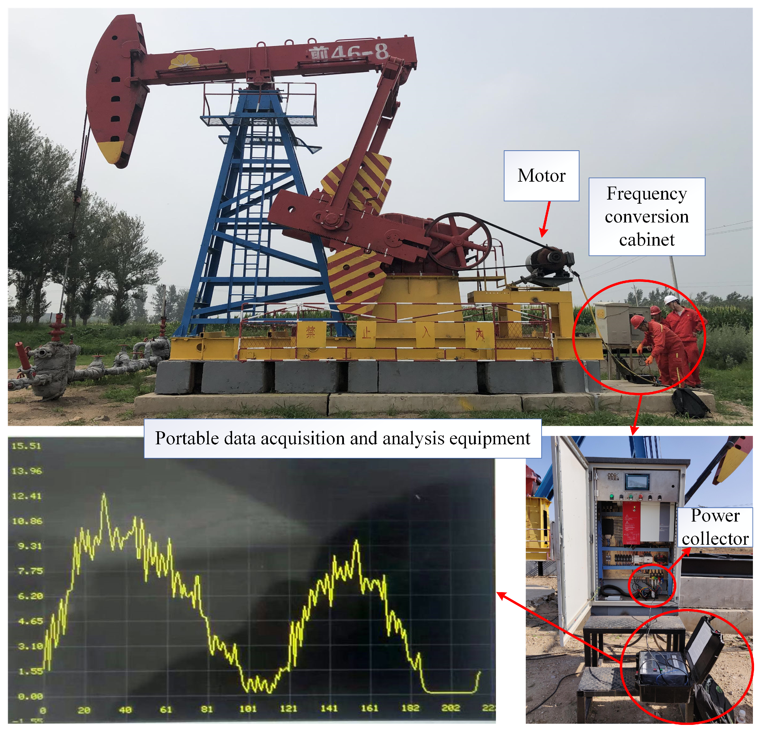
4.1. Data Collection

As illustrated in Figure 5, the portable device developed by the authors’ team in Northeastern University implements the MPCs acquisition by collecting the three-phase current and voltage of the motor. The device consists of five core units as follows:

• Power acquisition unit: realize the motor power calculation with the help of the ATT7022B.
• Transmission unit: realize remote query and parameter adjustment on mobiles and computers.
• Human–machine interaction unit: a touch screen is equipped to facilitate parameter entry, data query, and data display.
• Data storage unit: it is used to store the collected and calculated data and parameters.
• Data processing unit: with the help of the XC7Z020CLG400 chip, it implements the core calculation, including the trained diagnostic model, device operation, etc.

After long-term practice, 300 groups of MPCs are collected from seven oil wells with the same mechanical parameters as shown in

Table 2. The main parameters of the test well.

Parameters	Value	Parameters	Value
Well	CYJ14-5-73HB	Moter	Y250M-6
$A_1$/mm	7000	n/min${}^{-1}$	4
$A_2$/mm	3110	$P_s$/atm	120
C/mm	5790	$P_d$/atm	180
B/mm	7210	${\gamma }_g$:${\gamma }_w$:${\gamma }_o$	0.1:0.2:0.2
G/mm	1460	$d_p$/mm	44
D/mm	3110	$d_r$/mm	22
R/mm	1270	$S_p$/mm ${}^2$	1520
$W_{ck}$/kg	5374	$\int l_i$/m	1600
$W_{cb}$/kg	5378	$\int M_i$/kg	5139.2
$W_{ub}$/kg	1229	$M_{mol}$/g·mol${}^{-1}$	16

. All simulations are implemented in the MATLAB and Pytorch framework and conducted on a workstation with a Core i7-9700K [email protected] GHz and a GTX2080TI GPU with 11-GB memory.

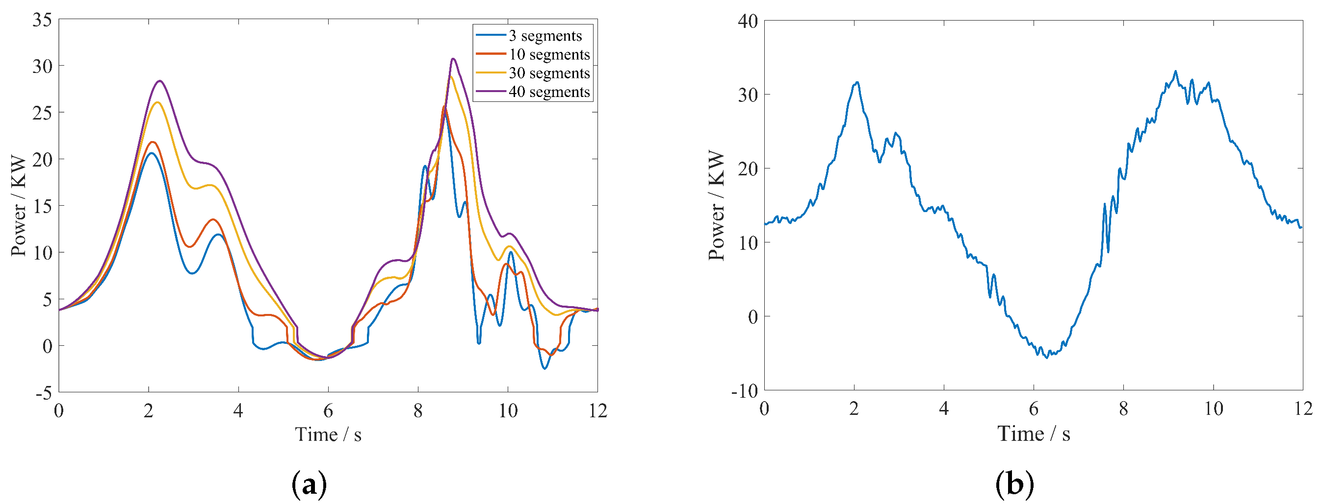
4.2. Validation of the Generated Motor Power Curves

According to the working and mechanical parameters listed in Table 2, the analysis results of six working conditions generated with the model in Section 2 are illustrated in Figure 6, Figure 7, Figure 8, Figure 9, Figure 10 and Figure 11. Each working state contains four sub-figures. The first sub-figures express the variation curves of the crucial variables in the pump containing the chamber volume, oil and water volume, the pressure, and the flow rate through the standing valve. The second and third sub-figures illustrate the generated DCs and MPCs under different working conditions. The fourth sub-figures are typical MPCs selected from the collected samples in practical scenarios.

As illustrated in the figures, the variation of essential parameters is consistent with the settings in Section 2.2. The characteristics embodied in the generated DCs under the different working conditions conform to the historical experience learned from the extensive data collected in different practical application scenarios. The generated and measured power curves have similar trends, and their characteristics are consistent with the previous mechanical analysis in Section 3.2.1. These results verify the rationality of the model on the mechanism analysis.

In order to take a more in-depth validity on the quantitative analysis, 50 samples of the MPCs under each working condition are generated as the training data by adjusting the downhole parameters to diagnose 300 groups of collected samples, which are testing data. The diagnostic method employs the mechanical feature extraction combined with the conditional random field (MCRF), which is mentioned in [6]. The experimental result is presented in Figure 12, where the diagnostic accuracy achieves 73% without the help of collected samples at all. This demonstrates the effectiveness of the generated data. However, the diagnostic accuracy does not meet the industrial requirement. The main reason mainly includes two aspects. On the one hand, limited by the insufficiency of the mechanism feature extraction method, some MPCs of critical working conditions are difficult to identify. On the other hand, the generated samples deviate from the actual samples’ distribution because of the model’s simplifications and interference in the data acquisition.

Moreover, the collected data are divided into two parts, where 240 groups are randomly selected as the training set, and the remaining 60 groups are the testing set. To comprehensively investigate the generated data, we set various scenarios with different amounts of generated samples adding to the training set of the collected data to monitor the working conditions in the SRPS. Three methods named 1-D CNN, CNN, and MCRF are selected from three perspectives of time-series, image, and mechanism to conduct experiments. The diagnostic results are shown in

Table 3. Diagnostic results with different amount of generated samples.

Method	A	B	C	D	E
Collected samples	0	240	240	240	240
Generated samples	300	0	150	300	450
1-D CNN	0.747	0.863	0.907	0.933	0.94
CNN	0.713	0.843	0.883	0.90	0.9133
MCRF	0.733	0.837	0.883	0.893	0.9067

.

As illustrated in Table 3, the diagnosis accuracy presents an upward trend as the generated samples are added to the original training set. Machine learning is more capable of extracting features than mechanistic feature analysis, and the time-series-based approach is more applicable to the MPCs than the curves acting as pictures.

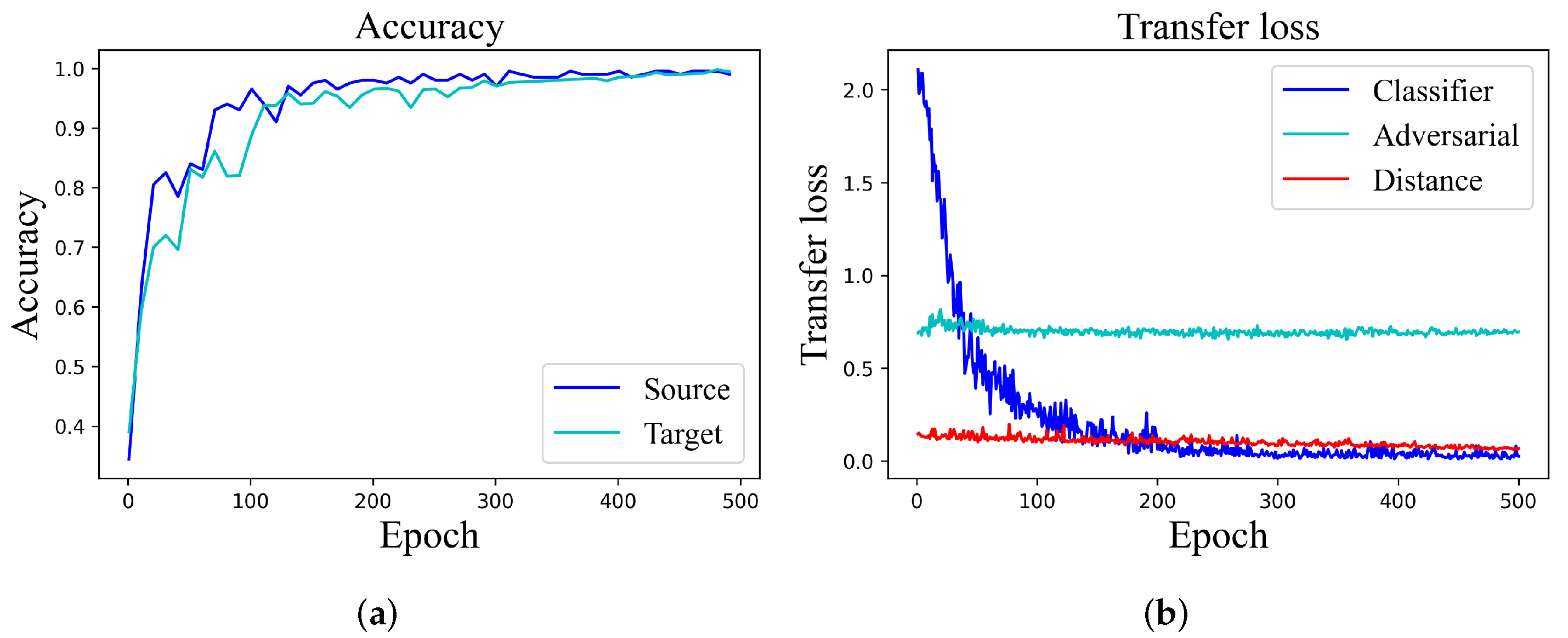
4.3. Diagnosis Based on Domain Adaptation

In this section, the proposed MADAN is employed to minimize the distribution discrepancy across domains in practical application scenarios. Since the new conditional metrics and pseudo-label learning strategy are appended to the objective function for the distribution alignment, the convergence analysis is imperative to illustrate the stability and transfer ability. As shown in Figure 13a, the discrepancy in diagnostic accuracy between the source and target domain gradually decreases with the iteration of optimization, which illustrates the effectiveness of the feature generator network in bridging the distribution discrepancy. In addition, the accuracy curves converge rapidly and finally approach 1, which demonstrates the superiority of this method in industrial diagnosis.

Furthermore, the training loss including classification loss (classifier_loss), domain classifier error (adversarial_loss), and conditional distribution loss (distance_loss) are plotted in Figure 13b, respectively. It can be found that the classification loss is gradually decreasing with the increasing of training epoch and finally approaches 0. The reciprocal oscillation of the adversarial loss illustrates that the domain classifier efficiently guides the feature generator network to explore domain-invariant features. This is because the feature extraction network keeps improving the information extraction capability under the requirement of the classifier error reduction, which makes the domain classifier keep improving the ability to discriminate domain features to inhibit the feature extraction network from retaining domain-related information. The conditional distribution loss presents a gradual declining trend. This demonstrates that the conditional distribution discrepancy is gradually disappearing.

For comparison purposes, several state-of-the-art methods are considered for comparisons with the MADAN, including 1-D CNN, DANN [21], DATLN [22], DTN [30], and MiDAN [24]. In order to make a fair comparison, all the compared methods adopt the same 1-D CNN architectures to explore features. The details of the compared methods are presented in

Table 4. Detailed description of the compared methods.

Method	MDA	CDA	Pseudo-Labels
1-D CNN	/	/	/
DANN	MMD	/	/
DATLN	MMD + Adversail	/	/
DTN	MMD	MMD	Pre-train network
MiDAN	Adversail	MMD	Pre-train network
MADAN (ours)	Adversail	MMD	Mechanism + Classifier

, where MDA denotes the marginal distributions alignment and CDA denotes the conditional distributions alignment.

The diagnostic result is an average of five random tests, where the testing set is 60 groups randomly split from the 300 groups of collected MPCs. To comprehensively show the capabilities of the proposed method, three evaluation indicators including Accuracy, F1-score, and MCC are selected to assess the performance of each method. The expressions of the MCC are defined as follows:

$$MCC=\frac{TN\times TP-FN\times FP}{\sqrt{(TF+TP)(FN+TN)(TP+FN)(FP+TN)}}.$$

(22)

The results are listed in

Table 5. Comparison research under various methodologies.

Method	Accuracy (%)	F1 (%)	MCC (%)
1-D CNN	83.33	83.25	79.9
DANN	91.67	91.38	89.69
DATLN	92.33	92.17	90.58
DTN	95.33	95.34	94.39
MiDAN	97	97.03	96.42
MADAN (ours)	98.33	98.51	98.17

.

As the results show, the MADAN performs better than other diagnostic methodologies in all evaluation indicators. Concretely, t-distributed stochastic neighbor embedding (t-SNE) is employed to demonstrate visual insights into the distribution discrepancy of features distilled by different methods from the generated and collected MPC. The t-SNE visualization for the original data and the features after the alignment by the methods mentioned above are illustrated in Figure 14.

From Table 5 and Figure 14, some results can be clearly obtained. Firstly, in terms of classification performance, the outlier source samples are much less with the help of transfer learning. In addition, the MADAN can better cluster the same categories and separate different categories than the other methods. Secondly, in terms of the marginal distributions alignment, the adversarial training is superior to the MMD, where Figure 14c,e correspond to Figure 14b,d, respectively. Thirdly, in terms of the conditional distributions alignment, the data in different domains within each category are more evenly distributed, where Figure 14d–f correspond to Figure 14a–c. Fourthly, in terms of pseudo-label learning, despite MiDAN having achieved good results, our MADAN performs better in the same number of iterations due to the higher pseudo-label accuracy resulting from assisted mechanisms during the initial training. From the analysis and discussion above, it can be seen that the proposed MADAN can effectively bridge the distribution discrepancy, resulting in better diagnosis performance in practical application scenarios.

5. Conclusions

The motor power as an easily collected signal contains information about the working status of the SRPS. In order to tackle the issue of an insufficiently labeled MPC database due to the early stage of the electrical parameters research on the SRPS, this paper has proposed an unsupervised fault diagnosis methodology named MADAN to leverage the generated MPCs of different working conditions to diagnose the actual MPCs. Firstly, an integrated dynamics mathematical model has been established to generate the MPCs under different working conditions. Secondly, a mechanism-assisted pseudo-label learning strategy and a conditional distribution discrepancy metric have been added to the adversarial domain adaptation model to bridge the marginal and conditional distribution discrepancy of the generated and collected MPCs. Finally, a set of actual MPCs collected by self-developed portable devices has been utilized to verify the feasibility of the proposed methodology. The experimental results indicated that the generated and the actual MPCs had similar trends, and the MADAN can effectively utilize the generated and actual unlabeled MPCs to realize the power fault diagnosis of oil wells.

References

1. Lv, X.; Wang, H.; Zhang, X.; Liu, Y.; Jiang, D.; Wei, B. An evolutional SVM method based on incremental algorithm and simulated indicator diagrams for fault diagnosis in sucker rod pumping systems. J. Pet. Sci. Eng. 2021, 203, 108806. [Google Scholar] [CrossRef]
2. Han, Y.; Song, X.; Li, K.; Yan, X. Hybrid modeling for submergence depth of the pumping well using stochastic configuration networks with random sampling. J. Pet. Sci. Eng. 2022, 208, 109423. [Google Scholar] [CrossRef]
3. Li, K.; Han, Y.; Wang, T. A novel prediction method for down-hole working conditions of the beam pumping unit based on 8-directions chain codes and online sequential extreme learning machine. J. Pet. Sci. Eng. 2018, 160, 285–301. [Google Scholar] [CrossRef]
4. Han, Y.; Li, K.; Ge, F.; Wang, Y.; Xu, W. Online fault diagnosis for sucker rod pumping well by optimized density peak clustering. ISA Trans. 2021, 120, 222–234. [Google Scholar] [CrossRef] [PubMed]
5. Takacs, G.; Kis, L. A new model to find optimum counterbalancing of sucker-rod pumping units including a rigorous procedure for gearbox torque calculations. J. Pet. Sci. Eng. 2021, 205, 108792. [Google Scholar] [CrossRef]
6. Zheng, B.; Gao, X.; Pan, R. Sucker rod pump working state diagnosis using motor data and hidden conditional random fields. IEEE Trans. Ind. Electron. 2019, 67, 7919–7928. [Google Scholar] [CrossRef]
7. Wei, J.; Gao, X. Fault Diagnosis of Sucker Rod Pump Based on Deep-Broad Learning Using Motor Data. IEEE Access 2020, 8, 222562–222571. [Google Scholar] [CrossRef]
8. Zhang, B.; Gao, X.; Li, X. Complete Simulation and Fault Diagnosis of Sucker-Rod Pumping. SPE Prod. Oper. 2021, 36, 277–290. [Google Scholar]
9. Zheng, B.; Gao, X.; Li, X. Fault detection for sucker rod pump based on motor power. Control Eng. Pract. 2019, 86, 37–47. [Google Scholar] [CrossRef]
10. Chen, L.; Gao, X.; Li, X. Using the motor power and XGBoost to diagnose working states of a sucker rod pump. J. Pet. Sci. Eng. 2021, 199, 108329. [Google Scholar] [CrossRef]
11. Gibbs, S. Predicting the behavior of sucker-rod pumping systems. J. Pet. Technol. 1963, 15, 769–778. [Google Scholar] [CrossRef]
12. Zheng, B.; Gao, X.; Li, X. Diagnosis of sucker rod pump based on generating dynamometer cards. J. Process Control 2019, 77, 76–88. [Google Scholar] [CrossRef]
13. Lv, X.; Wang, H.; Liu, Y.; Chen, S.; Lan, W.; Sun, B. A novel method of output metering with dynamometer card for SRPS under fault conditions. J. Pet. Sci. Eng. 2020, 192, 107098. [Google Scholar] [CrossRef]
14. Zhao, Z.; Zhang, Q.; Yu, X.; Sun, C.; Wang, S.; Yan, R.; Chen, X. Applications of Unsupervised Deep Transfer Learning to Intelligent Fault Diagnosis: A Survey and Comparative Study. IEEE Trans. Instrum. Meas. 2021, 70, 1–28. [Google Scholar] [CrossRef]
15. Zhang, W.; Li, X.; Ma, H.; Luo, Z.; Li, X. Open-Set Domain Adaptation in Machinery Fault Diagnostics Using Instance-Level Weighted Adversarial Learning. IEEE Trans. Ind. Inf. 2021, 17, 7445–7455. [Google Scholar] [CrossRef]
16. Ainapure, A.; Siahpour, S.; Li, X.; Majid, F.; Lee, J. Intelligent Robust Cross-Domain Fault Diagnostic Method for Rotating Machines Using Noisy Condition Labels. Mathematics 2022, 10, 455. [Google Scholar] [CrossRef]
17. Zhang, H.; Ren, H.; Mu, Y.; Han, J. Optimal Consensus Control Design for Multiagent Systems with Multiple Time Delay Using Adaptive Dynamic Programming. IEEE Trans. Cybern. 2021. [Google Scholar] [CrossRef]
18. Wen, L.; Gao, L.; Li, X. A new deep transfer learning based on sparse auto-encoder for fault diagnosis. IEEE Trans. Syst. Man Cybern. Syst. 2017, 49, 136–144. [Google Scholar] [CrossRef]
19. Ye, Z.; Yu, J.; Mao, L. Multisource Domain Adaption for Health Degradation Monitoring of Lithium-Ion Batteries. IEEE Trans. Transp. Electrif. 2021, 7, 2279–2292. [Google Scholar] [CrossRef]
20. Zhao, B.; Zhang, X.; Zhan, Z.; Wu, Q. Deep multi-scale separable convolutional network with triple attention mechanism: A novel multi-task domain adaptation method for intelligent fault diagnosis. Expert Syst. Appl. 2021, 182, 115087. [Google Scholar] [CrossRef]
21. Ganin, Y.; Ustinova, E.; Ajakan, H.; Germain, P.; Larochelle, H.; Laviolette, F.; Marchand, M.; Lempitsky, V. Domain-adversarial training of neural networks. J. Mach. Learn. Res. 2016, 17, 2030–2096. [Google Scholar]
22. Guo, L.; Lei, Y.; Xing, S.; Yan, T.; Li, N. Deep convolutional transfer learning network: A new method for intelligent fault diagnosis of machines with unlabeled data. IEEE Trans. Ind. Electron. 2018, 66, 7316–7325. [Google Scholar] [CrossRef]
23. Cheng, C.; Zhou, B.; Ma, G.; Wu, D.; Yuan, Y. Wasserstein distance based deep adversarial transfer learning for intelligent fault diagnosis with unlabeled or insufficient labeled data. Neurocomputing 2020, 409, 35–45. [Google Scholar] [CrossRef]
24. Tan, Y.; Guo, L.; Gao, H.; Lin, Z.; Liu, Y. MiDAN: A framework for cross-domain intelligent fault diagnosis with imbalanced datasets. Measurement 2021, 183, 109834. [Google Scholar] [CrossRef]
25. Li, Y.; Song, Y.; Jia, L.; Gao, S.; Li, Q.; Qiu, M. Intelligent fault diagnosis by fusing domain adversarial training and maximum mean discrepancy via ensemble learning. IEEE Trans. Ind. Inf. 2020, 17, 2833–2841. [Google Scholar] [CrossRef]
26. Li, X.; Zhang, W. Deep Learning-Based Partial Domain Adaptation Method on Intelligent Machinery Fault Diagnostics. IEEE Trans. Ind. Electron. 2021, 68, 4351–4361. [Google Scholar] [CrossRef]
27. Zhang, W.; Li, X.; Ma, H.; Luo, Z.; Li, X. Universal domain adaptation in fault diagnostics with hybrid weighted deep adversarial learning. IEEE Trans. Ind. Inf. 2021, 17, 7957–7967. [Google Scholar] [CrossRef]
28. Long, M.; Wang, J.; Ding, G.; Sun, J.; Yu, P.S. Transfer feature learning with joint distribution adaptation. In Proceedings of the IEEE International Conference on Computer Vision, Sydney, Australia, 2–8 December 2013; pp. 2200–2207. [Google Scholar]
29. Li, X.; Zhang, W.; Xu, N.X.; Ding, Q. Deep learning-based machinery fault diagnostics with domain adaptation across sensors at different places. IEEE Trans. Ind. Electron. 2019, 67, 6785–6794. [Google Scholar] [CrossRef]
30. Han, T.; Liu, C.; Yang, W.; Jiang, D. Deep transfer network with joint distribution adaptation: A new intelligent fault diagnosis framework for industry application. ISA Trans. 2020, 97, 269–281. [Google Scholar] [CrossRef] [Green Version]
31. Lu, N.; Xiao, H.; Sun, Y.; Han, M.; Wang, Y. A new method for intelligent fault diagnosis of machines based on unsupervised domain adaptation. Neurocomputing 2021, 427, 96–109. [Google Scholar] [CrossRef]
32. Liu, Y.; Zhong, L.; Qiu, J.; Lu, J.; Wang, W. Unsupervised Domain Adaptation for Nonintrusive Load Monitoring Via Adversarial and Joint Adaptation Network. IEEE Trans. Ind. Inf. 2022, 18, 266–277. [Google Scholar] [CrossRef]
33. Ganin, Y.; Lempitsky, V. Unsupervised domain adaptation by backpropagation. In Proceedings of the International Conference on Machine Learning, PMLR, Lille, France, 6–11 July 2015; pp. 1180–1189. [Google Scholar]
Figure 1. Sucker rod pump system.
Mathematics 10 01224 g001
Figure 2. The comparison between the actual and generated MPCs with different segments of the rod. (a) Generated power curves. (b) Actual power curve.
Mathematics 10 01224 g002
Figure 3. The framework of the proposed approach.
Mathematics 10 01224 g003
Figure 4. Pseudo-label learning based on the mechanism analysis.
Mathematics 10 01224 g004
Figure 5. A self-developed data acquisition and analysis equipment employed in the SRPS.
Mathematics 10 01224 g005
Figure 6. Normal working state. (a) Pump simulation. (b) Generated DC. (c) Generated MPC. (d) Actual MPC.
Mathematics 10 01224 g006
Figure 7. Traveling valve leakage working state. (a) Pump simulation. (b) Generated DC. (c) Generated MPC. (d) Actual MPC.
Mathematics 10 01224 g007
Figure 8. Insufficient liquid supply working state. (a) Pump simulation. (b) Generated DC. (c) Generated MPC. (d) Actual MPC.
Mathematics 10 01224 g008
Figure 9. Gas affected working state. (a) Pump simulation. (b) Generated DC. (c) Generated MPC. (d) Actual MPC.
Mathematics 10 01224 g009
Figure 10. Gas locking working state. (a) Pump simulation. (b) Generated DC. (c) Generated MPC. (d) Actual MPC.
Mathematics 10 01224 g010
Figure 11. Parting rod working state. (a) Pump simulation. (b) Generated DC. (c) Generated MPC. (d) Actual MPC.
Mathematics 10 01224 g011
Figure 12. The confusion matrices of diagnosis result.
Mathematics 10 01224 g012
Figure 13. The trend of training accuracy and loss on the MADAN. (a) Accuracy. (b) Loss.
Mathematics 10 01224 g013
Figure 14. T-SNE feature visualization. (a) Source sample. (b) 1-D CNN. (c) DANN. (d) DATLN. (e) DTN. (f) MiDAN. (g) MADAN (ours).
Mathematics 10 01224 g014