A Branch-and-Bound Algorithm for Minimizing the Total Tardiness of Multiple Developers

Abstract

In the game industry, tardiness is an important issue. Unlike a unifunctional machine, a developer may excel in programming but be mediocre in scene modeling. His/her processing speed varies with job type. To minimize tardiness, we need to schedule these developers carefully. Clearly, traditional scheduling algorithms for unifunctional machines are not suitable for such versatile developers. On the other hand, in an unrelated machine scheduling problem, n jobs can be processed by m machines at n × m different speeds, i.e., its solution space is too wide to be simplified. Therefore, a tardiness minimization problem considering three job types and versatile developers is presented. In this study, a branch-and-bound algorithm and a lower bound based on harmonic mean are proposed for minimizing the total tardiness. Theoretical analyses ensure the correctness of the proposed method. Computational experiments also show that the proposed method can ensure the optimality and efficiency for n ≤ 18. With the exact algorithm, we can fairly evaluate other approximate algorithms in the future.

1. Introduction

Game development is a complicated professional domain in which three limited resources, i.e., money, manpower, and time, have to be carefully managed. First, we should note that the cost of developing a multimedia game, e.g., an online game, is rising. The budget for developing a commercial multi-player game is at least $1,000,000. For some large-scale games, e.g., Grand Theft Auto V, developing a single version may even cost a company around $10,000,000 [1,2,3,4]. But once a successful game is released, it might earn a billion dollars in profit, e.g., [5,6]. In light of the above observations, game development involves considerable expertise, such as product planning, graphic design, sound design, programming, and testing. To avoid endless budget amendments, it is essential to carefully schedule all the jobs at the beginning.

Such a large game cannot be implemented by a single developer, making good teamwork another essential factor. A small-sized game may be implemented by a single designer. However, for some large-scale multimedia games, the team size may range from 3 to 100 professionals [7,8]. Each game draws upon various areas of expertise. For instance, a single piece of music requires various professional skills, e.g., composing, songwriting, dubbing, and sound effects. The professionals with these skills are sourced from different kinds of personnel pools. Some may be official company employees, while others may be temporarily recruited freelancers. Clearly, semi-finished products made by the former must be passed to the latter on schedule. If a critical job is delayed, it may leave dozens of professionals idle. Since their wages, hotel expenses, and dining fees need to be paid even during such an idle period, such costly human resources need to be carefully scheduled in advance.

The third major resource is time. These multimedia games must eventually be released onto the market, so game developers have to race against time to finish them as early as possible. Since these developers have various areas of expertise, their time costs are different. Consider two developers, Mary and Tom. Mary may be highly proficient at figure design, while Tom may excel in scene design. There are 100 figure design jobs, and both developers are qualified for these jobs. Any daily delay of a job will result in a $100 penalty. Consider further that Mary requires 30 person-days and charges $50,000; Tom takes 50 person-days and charges $30,000. To whom should we assign these jobs? How does a delayed job affect the following jobs? These jobs must be carefully scheduled in the beginning. Any delay in a critical job may cause serious damage. For scheduling such a project, the cost, time, and expertise should be considered as a whole. Clearly, it is not easy to solve such a scheduling problem by labor-intensive means. That is, such a scheduling problem in the game industry is no less challenging than those in the aviation, semiconductor, and construction industries.

In light of the above observations, it is clear that tardiness minimization is important in the game industry. In general, the jobs in a large multimedia game have various properties and different tolerance degrees to delay. For example, the job of leading figure design should be completed as early as possible—such an urgent job had better not be delayed. Conversely, late poster design or user manual translation may not cause a huge loss. If possible, all the jobs would best be completed on time. However, as in other industries, it is difficult to schedule more than 20 jobs manually. Therefore, tailored scheduling algorithms for reducing tardiness in the game industry are called for.

Assigning similar jobs to a developer with corresponding expertise helps to reduce tardiness. With the continued refinement of the game industry, developers specialize in different areas of expertise. Let us consider the above example again. Mary should be assigned figure design jobs, and Tom, scene design jobs. However, there are still some other constraints. Suppose that Mary is overloaded with a lot of figure design jobs. Although Mary is highly proficient at figure design, we had better assign some figure design jobs to Tom. Clearly, the computation of such trade-offs is very complicated. This is because multi-specialty developers are not taken into account in traditional scheduling models. Again, some new algorithms for scheduling such jobs and developers in the game industry are needed.

The following three properties distinguish the presented problem from traditional ones. First, for traditional heterogeneous machine scheduling problems, e.g., [9,10], a capable machine always outperforms others in terms of speed. However, for the presented problem, a developer may excel in figure design and programming but be mediocre in script design. That is, a single developer (or machine) simultaneously has both merits and shortcomings. It depends on what jobs are assigned to him/her. The considerations of the presented problem are more complicated than those of traditional heterogeneous machine scheduling problems.

Second, compared with identical machine scheduling problems, e.g., [11,12], the amount of computation of the presented problem is large. For m identical machines, we do not need to consider their permutations. Therefore, the solution space of the presented problem is about m! times larger than that of an identical machine scheduling problem. To our best knowledge, few researchers have focused their efforts on this emerging industry. However, the limited resources (i.e., money, time, and manpower) in this industry are seldom discussed.

Third, it is difficult to develop efficient lower bounds in a traditional unrelated machine scheduling problem, e.g., [13,14]. For n jobs, the processing speeds of m machines are all different; there are m × n various combinations, i.e., a large solution space. However, in most situations, a game developer usually processes his/her own desired jobs, i.e., one or two types. Such unrelated machine models are too complicated to schedule these developers in the game industry.

In this study, an optimization problem is presented. It is obvious that traditional scheduling algorithms cannot be directly applied to the problem. First, in unifunctional machine scheduling problems, a machine usually processes jobs at a fixed speed, e.g., a welding robot. In the presented problem, the processing speed is determined by the fitness between developers and job types. That is, the combinations that are needed to be considered become greater in number. Second, jobs with agreeable processing times and due dates, e.g., [15], are commonly employed to develop lower bounds and minimize tardiness. However, this technique will lead to an anomaly. Consequently, we propose an exact algorithm to schedule these various jobs and versatile developers in the game industry. Two main contributions are made in this study. First, a branch-and-bound algorithm is proposed for ensuring the optimality for n ≤ 18. Second, a lower bound based on a harmonic mean is developed to improve the execution efficiency.

The rest of this study is organized as follows. In the Section 2, past research is introduced. In the Section 3, the scheduling problem considering versatile developers is formulated. In the Section 4, a lower bound and a branch-and-bound algorithm are developed. In the Section 5, experiments are conducted to show the execution efficiency of the proposed algorithms. Conclusions are drawn in the Section 6.

2. Related Work

In this section, the motivations for tardiness minimization in the game industry are introduced. Moreover, the differences between the presented problem and traditional ones are also discussed.

2.1. Game Industry

Game development requires effective control of manpower, money, and time. Manpower plays a vital role in this industry. Unlike ordinary industries (e.g., lumbering), the modern game industry is dependent on versatile developers cooperating to develop their products. These developers may be first-party designers (e.g., Nintendo), second-party developers (e.g., [16]), or even third-party participants (e.g., [17,18,19]). Each of them may be multi-functional, able to deal with several kinds of jobs. This implies that scheduling these developers is more complicated than scheduling unifunctional machines in traditional industries. On the other hand, human resources in the game industry are expensive. From 2007 to 2018, the annual salaries of these developers increased from $66,000 to $73,000 [20,21]. Moreover, the team sizes range from a few to a hundred professionals, and the members of a team may be geographically distributed across two or three continents [7,8]. Although the scale of a game project is not always so large, the amount of computation for scheduling such a game project is still amazing. Especially for some critical jobs, tardiness can lead to heavy penalties [22,23]. Poorly managed projects may result in missed deadlines, cost overruns, reworking, or complaints. For more management failures, please refer to [24].

Incurring high costs is a not a rare phenomenon in the game industry. Due to advancements in technology, the plot of an online game may be more complicated than that of a motion picture, and the settings of a large game may be more fantastic than any scenic spot in the real world. Consequently, the costs of some well-known games, e.g., Call of Duty ($250 million), are higher than those of some science fiction films [1,25]. Moreover, a multimedia game is usually developed by a team instead of a single designer. Consequently, any delay may keep dozens of developers idle, which may entail further expenditures on wages, hotel expenses, and dining fees. In fact, due to bad control of budgets, most commercial games did not earn profits [7,26,27]. Such failures imply that effective budget control is an important issue in the game industry. For more information about game budgets and revenues, readers can refer to [2,3,4,5,6,8,28,29,30,31].

Time management is inevitable in the game industry. Both the game industry and traditional industries require massive capital investment, but the game industry has a special feature: time effectiveness. If a new house is 10 days late for the market, its price will not change greatly. However, if the official release of a commercial game is postponed and a rival gets ahead of the game, no players will consider the product of the loser because the novelty soon wears off. Moreover, with big data, we are able to predict or estimate a developer’s behaviors at the operational level easily. For example, all the technological processes of a developer can be observed and recorded, e.g., processing time, job type, failure probability; these data can be established as a database or a smart factory and such experiences can be repeatedly accessed and utilized [32,33,34]. In light of these observations, we learn that it becomes more possible and more necessary to punctually manage a large game project than before.

In summary, the game industry has grown to a considerable scale. It is impossible for a single designer to implement a large-scale multimedia game. Consequently, more efficient and effective management of manpower, money, and time is needed, rather than traditional labor-intensive tools.

2.2. Total Tardiness

In traditional multi-machine scheduling problems, the objective is usually to minimize the total tardiness, i.e., the sum of all jobs’ tardiness. Each job is tagged with a due date. Once a job is delayed, the objective cost increases. Moreover, in general, the tardiness of a job may lead to its successors’ tardiness. That is, there might be a ripple effect, in which the delay of a small job can affect the whole project. This means that the amount of computation of scheduling is huge, especially for multi-machine scheduling. For example, Mensendiek et al. [35] aimed to minimize the total tardiness of all the jobs on identical machines. They proposed a branch-and-bound algorithm for generating the optimal solutions and a metaheuristic algorithm, i.e., a genetic algorithm for obtaining approximate solutions. Due to the NP-hardness of this problem, the branch-and-bound algorithm performed well only for $n\le 18$, where n means the number of jobs. Wang [9] considered a total minimization problem on heterogeneous machines. A branch-and-bound algorithm was developed to ensure optimality for $n\le 18$. Note that m identical machines are much easier to schedule than m heterogeneous machines. For m identical machines, we only focus on how to permute n jobs, and we do not need to consider how to permute these identical machines. For example, in [13,36,37], they solved easier multi-machine scheduling problems. The reasons are stated as follows. First, since these machines are the same, the number of all the possible solutions for identical machines is just about 1/(m!) of that for heterogeneous machines. Second, each identical machine processes all jobs at a fixed speed. However, in our presented problem, a developer can perform jobs at different speeds. It depends on the type of each job. These differences imply that scheduling heterogeneous machines is more difficult. For more references to tardiness minimization, we can refer to [11,38,39,40,41].

Developing a large-scale game may involve thousands of jobs and hundreds of developers. Without proper scheduling algorithms, some jobs may be tardy. More seriously, a ripple effect will cause more jobs to be delayed. For example, tardiness will lead to low return rate and poor customer satisfaction [42,43]. Consequently, it is worthwhile to develop scheduling algorithms to minimize the total tardiness in the game industry.

2.3. Branch-and-Bound Algorithm

Branch-and-bound algorithms always generate the optimal solutions. These solution techniques are used for solving discrete and combinatorial optimization problems. Their great merit is their optimality, whereas their shortcoming is time consumption. Consequently, they are employed only for a small problem. For example, for using branch-and-bound algorithms to minimize total tardiness on a single machine, the maximal problem sizes for [44,45,46] are 18, 20, and 25, respectively. For minimizing the total tardiness on identical machines, the maximal problem sizes for [11,47] are 10, and 25, respectively. If machines are heterogeneous, the optimally solvable problem size of a branch-and-bound algorithm will decrease, e.g., n = 15 in [43] and n = 18 in [9]. This is because the solution space of a heterogeneous machine scheduling problem will be m! times larger than that of an identical machine scheduling problem. Even so, many researchers have focused on developing branch-and-bound algorithms in traditional industries. Unlike traditional industries, however, the modern game industry has various jobs and versatile developers. Namely, more efficient algorithms are needed for the complicated situation in the game industry. However, such exact algorithms are very time-consuming. For some tardiness minimization problems, e.g., an unrelated machine scheduling problem [48], their lower bounds were obtained by directly solving two max-min sub-problems, i.e., brute-force search. Consequently, some efficient lower bounds for accelerating branch-and-bound algorithms are also required.

Table 1. Comparisons between different scheduling environments.

Types	Unifunctional			Multi-Functional
Objective	Single Machine	Identical Machines	Heterogeneous Machines	Unrelated Machines	Versatile Developers
Tardiness	[44,45,46]	[47,50,51]	[9,43]	[48,52]	[this study]
Completion time	[53,54,55,56]	[57,58,59]		[60]
Makespan	[61,62]	[63]	[64]	[65]
Other objective	[49,66]	[67,68]	[69,70]

lists relevant studies that employ branch-and-bound algorithms to achieve their objectives in different environments. We divide these environments into two types: unifunctional machines and multi-functional ones. For example, a pump is a unifunctional machine used only for water distribution in [49]. Furthermore, branch-and-bound algorithms for scheduling unifunctional machines can be subdivided into three subtypes. First, the algorithms designed for a single machine are too simple to schedule multiple machines. Second, the branch-and-bound algorithms for identical machines still have their limitations, since they do not consider the permutations of different machines when optimizing. For example, since machines in [45] are identical, their position orders do not influence the design of a branch-and-bound algorithm. However, in this study, the situation is complicated by various developers. Third, even for heterogeneous machines, they process jobs of the same type only. For example, a powerful asphalt milling machines in [43] is still not able to lift containers. For each heterogeneous machine, only one fixed processing speed is considered. However, a developer in the game industry can process jobs of different types, e.g., programming and songwriting; hence, one developer may process jobs at several different paces. That is, a branch-and-bound algorithm for this study needs to search a larger solution space than other branch-and-bound algorithms for heterogeneous machines.

A multi-functional machine can process jobs of multiple types, i.e., different speeds. For unrelated machines, they can perform various jobs, and hence there are m × n different speeds, where m is the number of machines and n is the number of jobs. Suffering from no regular patterns summarized and deduced from such many relationships, some researchers had abandoned their attempt to develop an exact algorithm, e.g., [14]. Consequently, only a few studies focused on developing branch-and-bound algorithms for these unrelated machines. On the other hand, in the game industry, developers requiring preparations are relevant to unrelated machines with uncertain setup times. However, jobs regarding game development can be categorized into few types and only few relationships need to be taken into account. That is, an unrelated machine model is too complicated to develop an efficient lower bound. Some new exact algorithms for scheduling these versatile developers are thus required.

Moreover, the optimal solutions generated by branch-and-bound algorithms can be good benchmarks for evaluating metaheuristic algorithms. Despite the high number of jobs in game development, these jobs may be merely scheduled in Microsoft Excel or recorded in Google Calendar. Clearly, such a handmade itinerary is not qualified to be a benchmark for evaluating other methods. To our best knowledge, no researchers have investigated similar tardiness minimization problems in the game industry. A likely reason is that traditional grey-media PC games are simple and can be implemented by a few amateurs. Nowadays, however, the tide of the game industry is turning. Scheduling the jobs of a multimedia game project can be very complicated; hence, we need exact solutions to evaluate other metaheuristic algorithms.

3. Problem Formulation

The optimization problem is formulated as follows. There are n non-preemptive jobs and m developers. Each job j has a default processing time $p_j$, a due date $d_j$, and a job type $e_j\in \{1,2,3\}$ for $j=1,2,\dots ,n$. For each job type x, developer a has a processing difficulty ratio $r_{ax}$ for $a\in \{1,2,\dots ,m\}$ and $x\in \{1,2,3\}$. That is, if job j of type x (i.e., $e_j=x$) is assigned to developer a, the actual processing time is $p_j{r}_{ax}$. Each job needs to be assigned to one and only one developer, and each developer can process only one job at a time. On the other hand, if job j is assigned to developer a according to a schedule $\pi$, the actual completion time is denoted by $C_{j@a}(\pi )$ and the tardiness is defined by $T_{j@a}(\pi )=\max \{0,C_{j@a}(\pi )-d_j\}$. Under the above assumptions and constraints, we aim to determine an optimal schedule ${\pi }^{*}$ which minimizes the total tardiness; i.e., the minimization problem is defined by

$$\mathit{Minimize} f(\pi )={\displaystyle {\sum }_{a=1}^m{\displaystyle {\sum }_{j=1}^n{T}_{j@a}(\pi )}},$$

where $f(\pi )$ means the objective function.

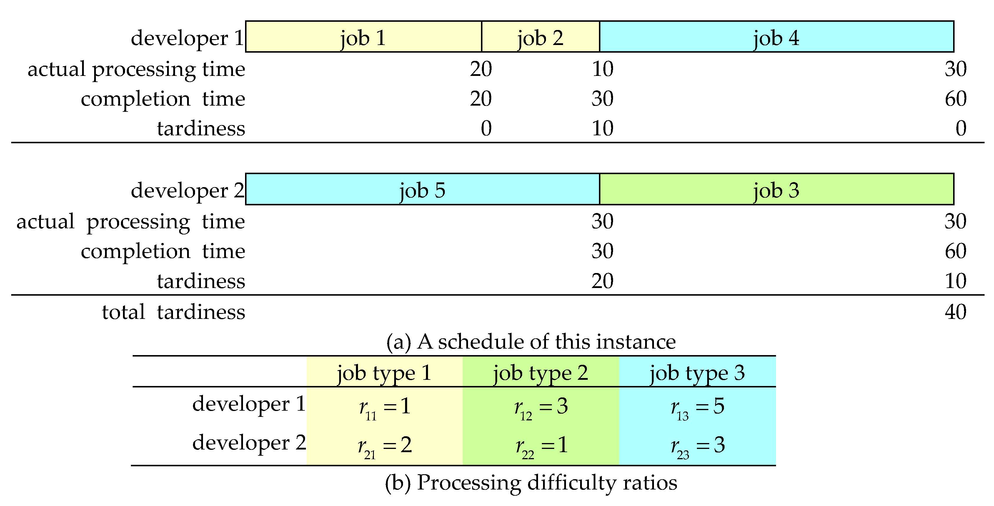
A problem instance is shown in Figure 1a. Let n = 5, m = 2, $p_j$ = 20, 10, 30, 6, 10, $d_j$ = 20, 20, 50, 70, 10, and $e_j$ = 1, 1, 2, 3, 3, for $j$ = 1, 2, 3, 4, 5. The processing difficulty ratios are listed in Figure 1b. Let $\pi =(1,2,4,0,5,3)$ be a schedule, where number 0 means a separator used to divide jobs between developers. Since developer 1 is highly proficient at dealing with jobs of type 1, job 1 and job 2 are assigned to developer 1, and their processing times are 20 and 10, respectively. Similarly, since developer 2 excels at processing jobs of type 2, job 3 is processed by developer 2, and its actual processing time is 30. Note that neither developer is skilled in processing jobs of type 3 (i.e., jobs 4 and 5). Since job 5 has an early due date, let developer 2 process it first, and its actual processing time is 30 (= 10 × $r_{23}$ = 10 × 3). Similarly, developer 1 requires a processing time of 30 (= 6 × $r_{13}$ = 6 × 5) to process job 5. Eventually, the total tardiness is $f(\pi )$ = 40 (i.e., 0 + 10 + 10 + 0 + 20).

It is clear that the above scheduling problem is different from traditional ones. The following features differentiate the presented problem from traditional ones:

• Compared with traditional unrelated machine scheduling problems, the concept of job type can reduce the amount of computation. For example, all the relationships between machines and jobs must be taken into account, e.g., the probability of machine i processing job j (p_ij) in [13] and the processing time of machine i processing job j (p_ij) in [14]. All the m × n combinations must be considered. If a job set is not given, blindly estimating each machine’s average processing speed cannot determine a good lower bound. However, in the presented problem, jobs can be categorized into three types and only m × 3 processing speeds are considered and their average processing speeds can be employed to develop a lower bound.
• In past heterogeneous machine scheduling models [41,69,71], a capable developer (or machine) always outperforms others in terms of processing speed. That is, each heterogeneous machine has its own fixed speed. However, in this presented problem, a developer might be mediocre in processing jobs of type 1 but excel in dealing with jobs of other types. Clearly, these developers cannot be modeled by such unifunctional machines.
• Compared with traditional identical machine scheduling problems, e.g., [11,12], the presented problem is more difficult. An example is given in

  Table 2. The number of all possible schedules.

  Job Assignment	Number of Possible Schedules
  one developer takes three jobs; two developers are idle	${\mathrm{C}}_1^{3}3!$
  one developer takes two jobs and another one takes one job; the remaining one is idle	${\mathrm{C}}_1^{3}2!{\mathrm{C}}_1^{2}1!$
  each developer takes one job	${\mathrm{C}}_1^3{\mathrm{C}}_1^2{\mathrm{C}}_1^1$
  total	36

  . Consider that we allocate the three jobs to three identical machines. It is obvious that there is only one schedule, and it is just the optimal schedule; i.e., each machine takes one job. However, in the presented problem, a capable developer might take all three jobs to achieve optimality. Consequently, we need to check all the possible situations listed in Table 2 to determine the optimal schedule.
• Traditional tardiness minimization techniques cannot be directly applied to this problem. Jobs with larger processing difficulty ratios may take precedence over jobs with earlier due dates. In the presented problem, the processing difficulty ratio, processing time, and due date should be considered as a whole.

In light of the above observations, traditional scheduling algorithms cannot be directly applied to this problem, and a new optimization algorithm is thus required. That is, if a project meets the following two criteria, manpower can be arranged by such algorithms. First, a project is interdisciplinary and it recruits cross-domain workers, no matter what kinds of workers it needs, e.g., employee or freelancer. A developer may acquire several competencies and can perform several kinds of jobs in the project. Second, the performance pattern of each developer is known. That is, we have the big data of all developers and can estimate each one’s processing time for processing a given kind of job [32,33,34].

4. Branch-and-Bound Algorithm

In this section, we develop a branch-and-bound algorithm (named BB). To obtain the optimal schedules, BB will explore each search tree in the depth-first-search (DFS) order. Moreover, to deter us from exploring useless partial schedules, we also propose some dominance rules and develop a lower bound.

4.1. Dominance Rules

For convenience, we introduce some notations at the beginning of developing dominance rules. Let $\pi =(\alpha ,\beta )$ be an undetermined schedule, where $\alpha$ is a determined partial sequence and $\beta$ is the undetermined part. We wonder if there exists any better schedule ${\pi }^{\prime }$ that outperforms $\pi$. Consequently, some dominance rules are developed to prove our doubts. Since these rules are similar, we provide only the first proof.

Case I: Consider that jobs i and j are the last two jobs of $\alpha$ and both jobs are assigned to the same developer a. Let ${\pi }^{\prime }$ be the schedule obtained by only interchanging the last two jobs i and j in $\alpha$. For simplicity, let $C_{i@a}(\pi )=t_i$, $C_{j@a}({\pi }^{\prime })=t_j^{\prime }$, and $C_{j@a}(\pi )=t_j=C_{i@a}({\pi }^{\prime })=t_i^{\prime }$. In the following rules, both jobs i and j in $\pi$ are tardy. However, if we interchange both of them, their tardiness can be alleviated a little. In Rule 1, though both jobs are still tardy in ${\pi }^{\prime }$, their resulting tardiness is lower than $\pi$. In Rule 2, the interchange makes job j not tardy, i.e., the resulting tardiness is reduced.

Rule 1.

If $t_i>d_i$, $t_j>d_j$, $t_j^{\prime }>d_j$, $t_i^{\prime }>d_i$, and $t_i+t_j-t_i^{\prime }-t_j^{\prime }>0$, then ${\pi }^{\prime }$ dominates $\pi$.

Proof. 

We prove this property by showing $T_{i@a}(\pi )+T_{j@a}(\pi )$>$T_{i@a}({\pi }^{\prime })+T_{j@a}({\pi }^{\prime })$. That is,

$$\begin{gathered} T_{i@a}(\pi )+T_{j@a}(\pi ) \\ =(t_i-d_i)+(t_j-d_j) \\ =(t_i+t_j)-(d_i+d_j) \\ \hspace{1em}\hspace{1em}\hspace{1em}\hspace{1em}\hspace{1em}\hspace{1em}\hspace{1em}\hspace{1em}\hspace{1em}\hspace{1em}\hspace{1em}\hspace{1em}\hspace{1em}> (t_i^{\prime }+{t^{\prime }}_j)-(d_i+d_j) (\mathrm{since} t_i+t_j-t_i^{\prime }-t_j^{\prime }>0) \\ =(t_i^{\prime }-d_i)+(t_j^{\prime }-d_j) \\ =T_{i@a}({\pi }^{\prime })+T_{j@a}({\pi }^{\prime }). \end{gathered}$$

The proof is complete. □

Rule 2.

If $t_i>d_i$, $t_j>d_j$, $t_j^{\prime }\le d_j$, and $t_i+t_j-t_i^{\prime }>d_j$, then ${\pi }^{\prime }$ dominates $\pi$.

In the following four rules, job j is tardy and job i is not in $\pi$. Rules 3 and 4 show that job j can be done in time in ${\pi }^{\prime }$ and the resulting tardiness can be improved. In Rules 5 and 6, job j is still tardy in ${\pi }^{\prime }$, but the accumulated tardiness can be alleviated.

Rule 3.

If $t_i\le d_i$, $t_j>d_j$, $t_j^{\prime }\le d_j$, and $t_i^{\prime }\le d_i$, then ${\pi }^{\prime }$ dominates $\pi$.

Rule 4.

If $t_i\le d_i$, $t_j>d_j$, $t_j^{\prime }\le d_j$, $t_i^{\prime }>d_i$, and $t_j-t_i^{\prime }>d_j-d_i$, then ${\pi }^{\prime }$ dominates $\pi$.

Rule 5.

If $t_i\le d_i$, $t_j>d_j$, $t_j^{\prime }>d_j$, $t_i^{\prime }\le d_i$, and $t_i-t_i^{\prime }>0$, then ${\pi }^{\prime }$ dominates $\pi$.

Rule 6.

If $t_i\le d_i$, $t_j>d_j$, $t_j^{\prime }>d_j$, $t_i^{\prime }>d_i$, and $t_j-t_j^{\prime }-t_i^{\prime }>-d_i$, then ${\pi }^{\prime }$ dominates $\pi$.

Rule 7 lets the job with an earlier due date be processed first if both jobs, i.e., i and j, are not tardy in $\pi$. That is, both objective costs of ${\pi }^{\prime }$ and $\pi$ are the same, and we can stop searching for one of them.

Rule 7.

If $t_i^{\prime }\le d_i$, $t_j^{\prime }\le d_j$, and $d_j<d_i$, let ${\pi }^{\prime }$ dominate $\pi$.

Case II: Consider that job i is the last job of $\alpha$, which is assigned to developer a, and job j can be any undetermined job in $\beta$. Moreover, job i is also the last job assigned to developer a. For simplicity, let $C_{i@a}(\pi )=t_i$ and $e_j=y\in \{1,2,3\}$. In Rule 8, it would be wasteful to assign very few jobs to developer a. That is, he/she can accept some extra job in $\beta$ if no tardiness occurs.

Rule 8.

If $t_i+p_j{r}_{ay}\le d_j$, then ${\pi }^{\prime }$ dominates $\pi$.

Case III: Consider that job i is the last job of $\alpha$, which is assigned to developer a, and job j can be any undetermined job in $\beta$. Let $e_i=x\in \{1,2,3\}$, $e_j=y\in \{1,2,3\}$, and ${\pi }^{\prime }$ be the schedule obtained by interchanging job i in $\alpha$ and job j in $\beta$. For simplicity, let $C_{i@a}(\pi )=t_i$ and $C_{j@a}({\pi }^{\prime })=t_j^{\prime }$. In Rule 9, we interchange job i in $\alpha$ and job j in $\beta$ if job j is more urgent and the total tardiness will not deteriorate. In Rule 10, developer a is mediocre at processing jobs of type x but highly proficient at processing jobs of type y. On the other hand, all the remaining developers excel at dealing with jobs of type x and are mediocre at processing jobs of type y. Therefore, we interchange jobs i in $\alpha$ and j in $\beta$. Note that the total tardiness will not be worse in the case.

Rule 9.

If $e_i=e_j$, $p_i=p_j$, $d_j<d_i$, and $t_j^{\prime }\le d_j$, then ${\pi }^{\prime }$ dominates $\pi$.

Rule 10.

If $x\ne y$, $p_i{r}_{ax}>p_j{r}_{ay}$, $d_j\le d_i$, $t_i-d_i\ge t_j^{\prime }-d_j$, and $\max \{p_i{r}_{a+1,x},p_i{r}_{a+2,x},\dots ,p_i{r}_{mx}\}\le$ $\min \{p_j{r}_{a+1,y},p_j{r}_{a+2,y},\dots ,p_j{r}_{my}\}$, then ${\pi }^{\prime }$ dominates $\pi$.

The following lemma shows that each developer’s workload has a squeeze effect. That is, if there exists a developer whose workload is unreasonably heavy, then there must be another developer who has a relatively light workload. Due to space limitations, the following proofs can be found in Appendix A.

Lemma 1.

For a schedule $\pi$, if there exists a developer a whose maximum completion time is larger than ${\displaystyle {\sum }_{j=1}^n{\max }_{i=1}^m\left\{p_j{r}_{i{e}_j}\right\}/m+}{\max }_{i=1}^m\left\{{\max }_{j=1}^n\right\{p_j{r}_{i{e}_j}\left\}\right\}$, there exists another developer b whose maximum completion time is less than $({\displaystyle {\sum }_{j=1}^n{\max }_{i=1}^m\left\{p_j{r}_{i{e}_j}\right\}})/m$.

The following rule can help us to avoid some unnecessary searches if any developer is overloaded. If there exists a developer whose maximum completion time is unreasonably long, then we can remove a job from the overloaded developer and assign it to a half-loaded developer. That is, the previous schedule is dominated.

Rule 11.

For an optimal schedule ${\pi }^{*}$, each developer’s maximum completion time is less than or equal to ${\displaystyle {\sum }_{j=1}^n{\max }_{i=1}^m\left\{p_j{r}_{i{e}_j}\right\}}/m+{\max }_{i=1}^m\left\{{\max }_{j=1}^n\right\{p_j{r}_{i{e}_j}\left\}\right\}$.

4.2. Lower Bound

A lower bound is needed to avoid unnecessary searching if we are in the middle of a schedule that is dominated or outperformed by others. That is, after adding up the determined cost and the estimated cost of the remaining part, if the sum is still larger than the current minimal objective cost, we can abandon further searches for the remaining part. Consequently, the earlier we can stop useless searches, the more execution time we can save.

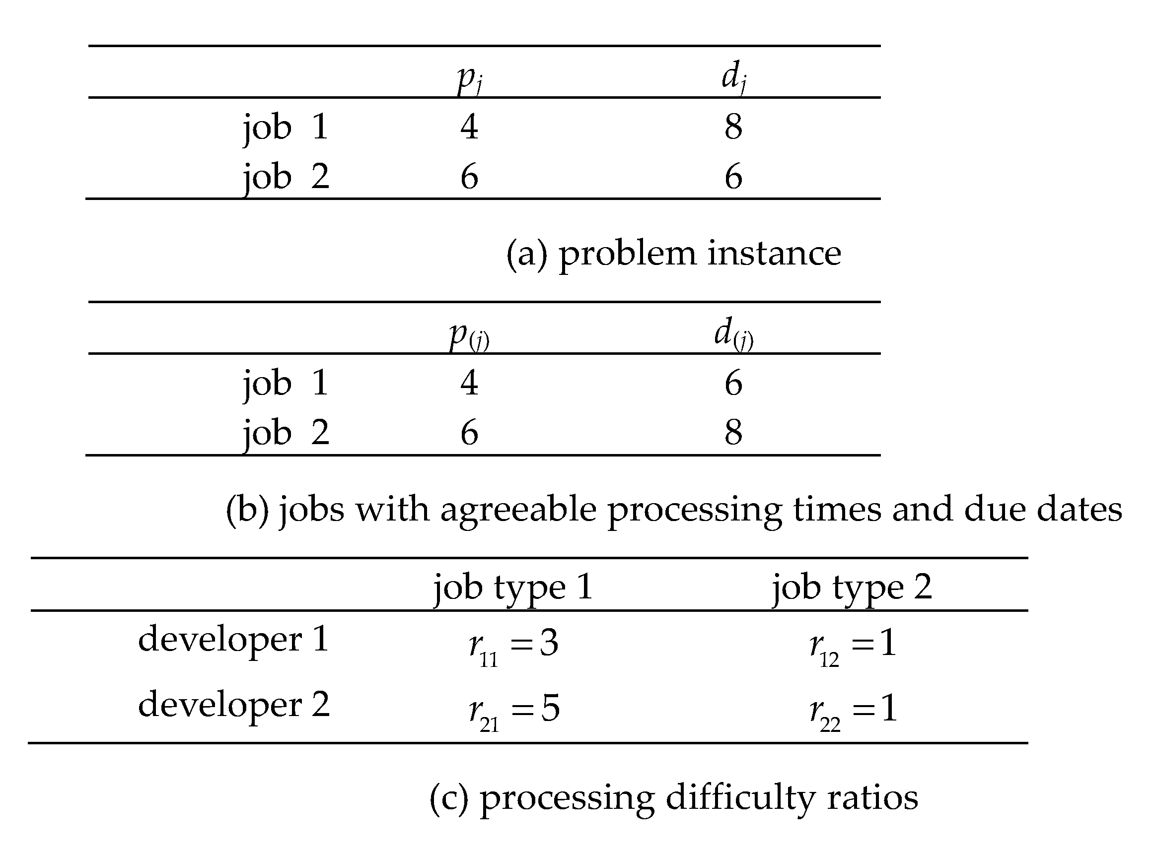
Arranging jobs with agreeable processing times and due dates is a useful way to obtain a lower bound for traditional tardiness minimization problems [15]. Here agreeableness is a kind of job correlation. As with precedence between two jobs in which a successor (e.g., testing) cannot start until a predecessor (e.g., programming) has finished, agreeableness between any two jobs implies that the smaller job (i.e., less processing time) always has an earlier due date, i.e., another kind of job correlation. However, it may lead to some anomalies in our problem. Consider that two identical developers (or machines) deal with the two jobs shown in Figure 2a. To obtain a lower bound, in Figure 2b, traditional algorithms may adjust the processing times and due dates and make them agreeable, i.e., $d_{(i)}\le d_{(j)}$ if and only if $p_{(i)}\le p_{(j)}$. Hence, the lower bound for these jobs is 0; i.e., max{0, 4 − 6} + max{0, 6 − 8}. However, in our problem, an anomaly occurs. Let $e_1=1$, $e_2=2$, and the processing difficulty ratios are shown in Figure 2c. For the original jobs shown in Figure 2a, the optimal objective cost is 4; i.e., max{0, 3 × 4 − 8} + max{0, 1 × 6 − 6}. For these virtual jobs shown in Figure 2b, the lower bound is 6; i.e., max{0, 3 × 4 − 6} + max{0, 1 × 6 − 8}. However, a lower bound is never larger than the minimal cost. Consequently, we cannot directly apply this technique here. In our problem, a job with a larger processing difficulty ratio may be more urgent than another with an earlier due date. That is, the processing times, due dates, and processing difficulty ratios should be considered as a whole in this problem.

Since these developers differ in their abilities (i.e., various processing difficulty ratios), we aim to fabricate an equivalent substitute to replace these heterogeneous developers in the real world. Consider that there are k different developers in the real world and assume that there are k virtually identical developers whose integrated ability is just equal to the sum of all the real ones’ abilities. The following definition gives the correct magnitude of processing difficulty ratio for each virtual developer. It is interesting that the magnitude is the harmonic mean of all the real developers’ processing difficulty ratios.

Definition 1.

There are k available developers numbered from m − k + 1 to m in the real world. Let there be k virtually identical developers. For each job type x, the equivalent processing difficulty ratio of each virtual developer is $k/(1/r_{m-k+1,x}+1/r_{m-k+2,x}+\dots +1/r_{mx})$and denoted by ${}_k\tilde{r}_x$.

The following lemma shows that the throughput (i.e., the amount of work per unit time) of these virtual developers is the same as the sum of all the real ones’ throughputs. For more information about harmonic mean, readers can refer to [72,73].

Lemma 2.

For a given job type x, the sum of the last k real developers’ throughputs (i.e., ${\displaystyle {\sum }_{a=m-k+1}^{m}1/r_{ax}}$) is equivalent to that of the k virtual ones’ throughputs (i.e., $k/{}_k\tilde{r}_x$).

Now we can merge these virtual developers into a virtual substitute. The following definition gives the correct magnitude of the processing difficulty ratio of the single substitute. Moreover, the following lemma shows that the throughput of the k virtual developers is exactly equal to that of the virtual single substitute.

Definition 2.

There are k available developers numbered from m − k + 1 to m in the real world. Let there be only one virtually equivalent developer, called the substitute. For each job type x, the processing difficulty ratio of the substitute is $1/(1/r_{m-k+1,x}+1/r_{m-k+2,x}+\dots +1/r_{mx})$and denoted by ${}_k\overline{r}_x$, i.e., ${}_k\overline{r}_x={}_k\tilde{r}_x/k$.

Lemma 3.

For a given job type x, the sum of the last k real developers’ throughputs (i.e., ${\displaystyle {\sum }_{a=m-k+1}^{m}1/r_{ax}}$) is equivalent to that of the substitute’s throughput (i.e., $1/{}_k\overline{r}_x$).

For each different job type, the virtual substitute still has different processing difficulty ratios. The following definition provides the upper and lower limits of the processing difficulty ratios for the substitute. The following lemma shows the boundary of the k real developers’ throughputs. This lemma guarantees that the throughput of the virtual substitute is larger than or at least equal to that of the k real developers.

Definition 3.

For each virtual developer transformed by k available real developers, let${}_k\overline{r}_{\min }=\min \{{}_k\overline{r}_1,{}_k\overline{r}_2,{}_k\overline{r}_3\}$and ${}_k\overline{r}_{\max }=\max \{{}_k\overline{r}_1,{}_k\overline{r}_2,{}_k\overline{r}_3\}$denote his/her minimal processing difficulty ratio and maximal processing difficulty ratio, respectively.

Lemma 4.

The throughput of the last k real developers is less than or equal to$1/{}_k\overline{r}_{\min }$.

Algorithm 1 shows the algorithm of the proposed lower bound (named LB). Note that BB explores a schedule $\pi =(\alpha ,\beta )$ in the DFS order. Since the jobs in $\alpha$ are determined, we let some job k be the last job of $\alpha$, i.e., $lj(\alpha )$=k, and some developer a process it, i.e., $ld(\alpha )$=a. Hence, there are $m-a$ available developers before $C_k(\pi )$. By Lemma 4, we can regard the $m-a$ developers as a virtual developer with processing speed $1/{}_{m-a}\overline{r}_{\min }$. Similarly, the $m-a+1$ developers before $C_k(\pi )$ can be viewed as another virtual developer with processing speed $1/{}_{m-a+1}\overline{r}_{\min }$. In Step 1, we determine which job is the last job in $\alpha$ and which developer completes the job. In Steps 2–3, the jobs in $\beta$ are transformed into $n-l$ new jobs whose processing times and due dates are agreeable, i.e., $p_{(i)}\le p_{(j)}$ if and only if $d_{(i)}\le d_{(j)}$. This modification ensures that such a lower bound will not be larger than the actual optimal cost [74,75]. Then we allocate these jobs to the two virtual developers at the pace of a unit job in Steps 5–14. We preemptively allocate the transformed jobs and start from time 0. If LB proceeds before time $C_k(\pi )$, we allocate the workload to the first virtual developer (Steps 9–10); otherwise, we let the second virtual developer process the remaining part (Steps 12–13). In Step 15, the estimated tardiness is accumulated, if any. Finally, the estimated lower bound is returned.

Algorithm 1. The proposed lower bound (LB($\pi$,$l$)).

INPUT

$\pi =(\alpha ,\beta )$, where $\alpha$ is a determined partial sequence and $\beta$ is the undetermined part

$l$ is the number of jobs in $\alpha$

OUTPUT

$cos{t}^{lb}$ is the lower bound for the current schedule $\pi =(\alpha ,\beta )$

(1) Set a = $ld(\alpha )$ and k = $lj(\alpha )$;

(2) Sort the processing times of the jobs in $\beta$ in ascending order, i.e., $p_{(j)}$ for j = 1 to n − l;

(3) Sort the due dates of the jobs in $\beta$ in ascending order, i.e., $d_{(j)}$ for j = 1 to $n-l$;

(4) Set $cos{t}^{lb}=f(\alpha )$ and currentTime=0;  //start to allocate the workload of $\beta$

(5) For $j=1$ to $n-l$ do Steps 6–15;

(6)    Set currentAmount=$p_{(j)}$;   //the amount of work of job (j)

(7)    Repeat Steps 8–14 until currentAmount=0;

(8)     If $currentTime<C_k(\pi )$ then do Steps 9–10;

(9)       Set $\Delta =\min \{currentAmount,1/{}_{m-a}\overline{r}{}_{\min }\}$;

(10)       Set $currentTime=currentTime+\Delta \times {}_{m-a}\overline{r}{}_{\min }$;

(11)     Else do Steps 12–13;

(12)       Set $\Delta =\min \{currentAmount,1/{}_{m-a+1}\overline{r}{}_{\min }\}$;

(13)       Set $currentTime=currentTime+\Delta \times {}_{m-a+1}\overline{r}{}_{\min }$;

(14)     Set $currentAmount=currentAmount-\Delta$;

(15)  Set $cos{t}^{lb}=cos{t}^{lb}+\max \{0,currentTime-d_{(j)}\}$;

(16) Output $cos{t}^{lb}$.

Theorem 1 shows the correctness of the proposed lower bound. By Theorem 1, the object cost of the substitute (i.e., the lower bound) will not be larger than the actual optimal cost in the real world.

Theorem 1.

Let $f({\pi }^{*})$be the optimal objective cost and $LB(\pi )$ be the lower bound. Then $f({\pi }^{*})\ge LB(\pi )$, where ${\pi }^{*}$ denotes the optimal schedule and $\pi$ denotes a schedule.

4.3. Branch-and-Bound Algorithm

Given the above dominance rules and lower bound, a branch-and-bound algorithm (named BB) is therefore developed and shown in Algorithm 2. The exact algorithm recursively explores the solution space in a DFS manner. Every time we enter the recursive algorithm, we check if the current partial sequence $\alpha$ of length l is dominated or the current lower bound is larger than the up-to-the-minute lowest cost (Step 1). If not, BB recursively calls itself (Steps 5–8). Since there are still $n-l+1$ undetermined jobs in $\beta$, we make $n-l+1$ new subsequences, and each starts with a different leading job. Then, we repeatedly replace the original $\beta$ and obtain $n-l+1$ new schedules (Steps 5–7). At the end, BB is recursively called by itself for $n-l+1$ times (Step 8). Note that both $cos{t}^{*}$ and ${\pi }^{*}$ are global variables. When the recursive algorithm ends, the globally optimal schedule and the minimal cost are stored in both of them.

Algorithm 2. The proposed branch-and-bound algorithm (BB($\pi$,$l$)).

INPUT

$\pi =(\alpha ,\beta )$, where $\alpha$ is a determined partial sequence and $\beta$ is the undetermined part

$l$ is the number of jobs in $\alpha$

OUTPUT

$cos{t}^{*}$ is the minimal cost //a global variable

${\pi }^{*}$ is the optimal schedule //a global variable

(1)  If ($\pi$ is not dominated and LB($\pi$,$l$)$\le cos{t}^{*}$) then do Steps 2–8;

(2)     If $l=n$ then do Step 3;

(3)      If $f(\pi )<cos{t}^{*}$ then set $cos{t}^{*}=f(\pi )$ and ${\pi }^{*}=\pi$;

(4)     Else do Steps 5–8;

(5)      For j = l + 1 to $n$ do Steps 6–8;

(6)        Set ${\pi }_0=\pi$;

(7)        Swap the ($l$+1)st and $j$th jobs of ${\pi }_0$;

(8)        Call BB(${\pi }_0$,$l$+1) recursively.

So far, we have proposed an exact algorithm named BB for locating the optimal solutions. With the aid of the dominance rules and lower bound, BB does not need to search for the entire solution space. Some dominated branches can be omitted, and the execution time is thereby reduced.

5. Experimental Results

In this section, we will observe the performance of the proposed branch-and-bound algorithm for n ≤ 18 and the efficiency of the proposed lower bound for n ≤ 12. Moreover, sensitivity tests are performed to show the influence of each control parameter. All the proposed algorithms are implemented in Pascal and executed on an Intel Core i7 @ 3.40 GHz with 8 GB RAM in a Windows 7 SP1 environment. For each setting, 50 random trials are conducted, and their execution times are measured in seconds. Finally, experimental results are discussed and compared.

5.1. Computational Results

We conduct experiments to observe the performance of BB and LB, and we show how the parameters (e.g., n) affect the objective costs of this problem.

Table 3. The parameters used in the experiments.

Parameter.	Default	Range	Meaning
$m$	3	$m\in \{3,4,\dots ,10\}$	the number of developers
$n$	15	$n\in \{12,15,18\}$	the number of jobs
$n_1:n_2:n_3$	1:1:1	$n_1,n_2,n_3\in \{1,2,3,4,6\}$	the ratios of numbers of three types of jobs
$m_1:m_2:m_3$	1:1:1	$m_1,m_2,m_3\in \{1,2\}$	the ratios of numbers of three kinds of developers
$p_j$		$p_j\in \{1,2,\dots ,100\}$	the default processing time of job j
$d_j$		$DU(T(1-\tau -R/2)/m,T(1-\tau +R/2)/m)$	the due date of job j
$\tau$	0.5	$\tau \in \{0.25,0.5,0.75\}$	a control parameter
$R$	0.5	$R\in \{0.25,0.5,0.75\}$	a control parameter

lists all the parameters used in this section. Parameters $m$, $n$, $p_j$, and $d_j$ have already been defined in Section 3. To model different job types, we let $n_j$ be the number of jobs of type $e_j$ for $j=1,2,3$, where $n_1+n_2+n_3=n$. To realize different processing difficulties, we let there be three kinds of developers in the following experiments. The first kind means average developers, i.e., $r_{ax}\in \{4,5,6,7\}$. The second kind means uni-specialty experts who excel in only one arbitrary job type, i.e., $r_{ax}\in \{1,2,3\}$; however, for the other two job types, their processing difficulty ratios are in $\{4,5,\dots ,10\}$. The third kind means bi-specialty experts who are highly proficient at two arbitrary job types with processing difficulty ratios less than or equal to 3; for the remaining job type, their processing difficulty ratios are in $\{4,5,\dots ,10\}$. Now we let $m_i$ be the number of the ith kind developers for $i=1,2,3$, where $m_1+m_2+m_3=m$. Moreover, we let T be the total default processing time and use $\tau$ and $R$ to control $p_j$ and $d_j$ such that they follow two discrete uniform distributions, respectively, i.e., $p_j~DU(1,100)$ and $d_j~DU(T(1-\tau -R/2)/m,T(1-\tau +R/2)/m)$.

For clarity, the experiments are divided into three parts. In the first part, we observe the performance of BB.

Table 4. The effects of different developers on the performance of BB for n = 12.

					Nodes		Run Time
m1	m2	m3	τ	R	Mean	Max	Mean	Max
1	1	1	0.25	0.25	18,370.78	181,419	0.06	0.50
				0.50	9593.32	212,150	0.04	0.51
				0.75	19,524.00	446,583	0.05	0.92
			0.50	0.25	39,897.70	1,232,184	0.10	2.22
				0.50	26,260.88	187,200	0.08	0.41
				0.75	56,571.82	897,059	0.14	1.73
			0.75	0.25	15,846.60	151,177	0.06	0.47
				0.50	96,882.38	888,828	0.21	1.65
2	1	1	0.25	0.25	101,401.70	910,464	0.36	3.35
				0.50	109,910.36	1,092,293	0.36	2.95
				0.75	97,957.36	802,617	0.33	2.47
			0.50	0.25	270,988.78	2,223,591	0.91	6.35
				0.50	176,245.60	1,806,727	0.66	5.88
				0.75	212,420.18	1,995,777	0.79	6.01
			0.75	0.25	298,785.28	3,410,329	1.07	10.55
				0.50	273,726.30	2,054,655	1.03	5.93
1	2	1	0.25	0.25	256,641.64	2,077,102	0.88	5.91
				0.50	74,059.52	1,132,219	0.24	3.21
				0.75	127,228.54	2,405,058	0.41	6.66
			0.50	0.25	257,390.84	1,437,686	0.97	5.18
				0.50	204,801.28	2,012,269	0.77	6.55
				0.75	130,780.72	1,637,102	0.50	5.43
			0.75	0.25	365,249.76	3,624,957	1.27	10.92
				0.50	286,986.04	3,464,396	1.12	10.34
1	1	2	0.25	0.25	61,395.10	1,368,806	0.20	4.40
				0.50	87,579.64	1,151,718	0.27	3.09
				0.75	35,620.74	457,695	0.12	1.62
			0.50	0.25	221,134.08	1,639,608	0.74	5.02
				0.50	159,399.06	1,401,974	0.59	4.45
				0.75	111,593.84	1,778,863	0.38	4.84
			0.75	0.25	183,150.22	1,821,915	0.75	5.52
				0.50	261,788.22	3,446,590	1.00	10.53

shows the performance of BB when the problem size is small, i.e., n = 12. Note that all the other parameters are set to their default values. Clearly, the execution time increases if we add an extra developer, no matter what kind of developer he/she is. It implies that m also affects the execution time. On the other hand, $\tau$ influences the execution time more greatly than R. When all the jobs have earlier due dates, i.e., a large $\tau$, each urgent job competes for limited resources, i.e., the m developers, more intensively. Consequently, BB will consume more execution time.

Table 5. The effects of different job types on the performance of BB for n = 12 and m = 3.

					Nodes		Run Time
n1	n2	n3	τ	R	Mean	Max	Mean	Max
4	4	4	0.25	0.25	18,370.78	181,419	0.06	0.47
				0.50	9593.32	212,150	0.03	0.52
				0.75	19,524.00	446,583	0.05	0.89
			0.50	0.25	39,897.70	1,232,184	0.10	2.14
				0.50	26,260.88	187,200	0.08	0.39
				0.75	56,571.82	897,059	0.14	1.70
			0.75	0.25	15,846.60	151,177	0.06	0.45
				0.50	96,882.38	888,828	0.20	1.67
6	3	3	0.25	0.25	48,235.18	610,127	0.10	1.08
				0.50	15,033.78	289,255	0.05	0.53
				0.75	30,411.54	810,984	0.08	1.62
			0.50	0.25	81,822.56	1,363,082	0.17	2.34
				0.50	86,449.52	1,937,334	0.19	3.43
				0.75	71,117.54	1,515,854	0.17	2.95
			0.75	0.25	56,112.42	599,630	0.14	1.16
				0.50	55,230.54	596,208	0.14	1.17
3	6	3	0.25	0.25	48,950.30	824,686	0.10	1.50
				0.50	41,753.44	718,820	0.10	1.40
				0.75	19,455.30	337,312	0.05	0.72
			0.50	0.25	27,156.02	498,306	0.06	0.97
				0.50	28,169.92	266,235	0.07	0.48
				0.75	96,447.08	1,073,225	0.20	1.92
			0.75	0.25	28,469.94	386,418	0.08	0.69
				0.50	17,570.98	161,400	0.07	0.36
3	3	6	0.25	0.25	77,097.48	1,825,223	0.15	3.17
				0.50	19,010.46	429,951	0.06	0.92
				0.75	10,107.86	118,662	0.03	0.33
			0.50	0.25	13,850.10	140,747	0.05	0.27
				0.50	34,581.10	615,020	0.09	1.26
				0.75	19,981.30	300,472	0.07	0.78
			0.75	0.25	62,164.04	645,173	0.15	1.14
				0.50	82,895.56	1,211,363	0.19	2.01

shows the performance of BB when we have a fixed number of developers, i.e., m = 3. For the fixed numbers of developers and jobs, job type does not affect BB’s performance. Even if there are only one job type and one developer type, BB will spend the same execution time to solve the problem. Unless all the m developers degenerate into the same developer type with the same processing difficulty or the n jobs degenerate into the same jobs with the same processing time and due date, the problem will not become easy.

Table 6. The effects of different developers on the performance of BB for n = 15.

					Nodes		Run Time
m1	m2	m3	τ	R	Mean	Max	Mean	Max	NA
1	1	1	0.25	0.25	832,453.28	17,232,335	2.23	40.61	0
				0.50	1,173,016.88	18,230,680	2.76	34.65	0
				0.75	2,839,962.76	90,961,123	6.37	186.42	0
			0.50	0.25	3,570,734.50	91,641,006	7.11	159.01	0
				0.50	1,172,994.72	29,159,216	2.99	57.91	0
				0.75	1,344,699.38	25,665,172	3.22	52.54	0
			0.75	0.25	1,585,250.42	45,125,597	3.27	84.97	0
				0.50	1,887,259.78	37,617,906	4.38	77.03	0
2	1	1	0.25	0.25	9,280,351.84	92,376,059	35.60	328.35	0
				0.50	11,525,379.06	76,888,161	43.80	245.14	0
				0.75	5,708,317.28	72,583,683	22.44	247.59	0
			0.50	0.25	12,132,170.62	70,022,775	52.61	247.34	3
				0.50	13,159,371.16	80,050,726	55.29	375.85	6
				0.75	6,812,266.80	44,382,802	30.67	178.57	0
			0.75	0.25	10,194,654.96	46,754,558	43.85	173.58	1
				0.50	12,479,543.60	85,937,662	53.63	317.48	3
1	2	1	0.25	0.25	7,337,408.85	87,562,414	28.12	297.81	3
				0.50	1,523,108.36	20,681,937	7.21	92.70	3
				0.75	3,289,152.32	48,793,151	13.53	215.75	0
			0.50	0.25	13,103,920.89	98,946,177	55.18	418.29	3
				0.50	7,720,935.63	76,197,365	34.11	250.87	2
				0.75	7,960,357.32	70,165,954	38.45	318.60	3
			0.75	0.25	12,444,367.94	94,805,781	60.85	399.64	2
				0.50	14,428,769.51	66,722,021	71.14	340.97	1
1	1	2	0.25	0.25	7,099,596.36	56,396,794	26.69	226.65	0
				0.50	2,039,534.46	33,925,880	8.72	168.64	0
				0.75	3,038,446.44	39,536,363	11.74	154.89	0
			0.50	0.25	3,089,474.55	31,463,439	14.45	135.10	1
				0.50	5,715,252.84	63,253,517	26.02	262.58	0
				0.75	3,938,160.00	82,372,316	18.97	371.99	1
			0.75	0.25	4,460,356.04	92,613,311	23.85	412.17	4
				0.50	9,424,598.91	93,532,752	48.06	410.98	5

shows the performance of BB when the problem size is medium, i.e., n = 15. At the beginning, we let the setting $m_1=m_2=m_3=1$ be a benchmark for later observations. The column of NA means the number of problem instances unsolved within a hundred million nodes. Again, the more developers we have, the more difficult the problem becomes. However, for all the settings with $m_1+m_2+m_3=4$, the results reveal that the problem instances having later due dates ($\tau =0.25$) are easier to solve. Most of them can be solved within a hundred million nodes.

Table 7. The effects of different developers on the performance of BB for n = 18.

					BB					GA
					Nodes		Run Time			Run Time		REP
m1	m2	m3	τ	R	Mean	Max	Mean	Max	NA	Mean	Max	Min	Max
1	1	1	0.25	0.25	5,762,157.45	81,285,117	23.74	332.25	1	0.02	0.03	99.47	3700.00
				0.50	3,628,152.57	40,038,729	15.61	142.29	3	0.02	0.05	2108.40	51,200.00
				0.75	4,071,432.28	55,782,442	18.53	301.04	4	0.02	0.05	1944.37	26,700.00
			0.50	0.25	8,719,240.57	83,839,140	26.00	209.26	4	0.02	0.03	14.35	65.52
				0.50	6,508,956.43	69,159,123	23.11	225.41	3	0.03	0.05	35.75	339.62
				0.75	5,836,731.36	46,618,119	21.49	144.13	5	0.03	0.05	65.80	733.33
			0.75	0.25	12,581,501.02	82,922,868	39.76	302.70	1	0.03	0.05	5.94	19.89
				0.50	7,687,742.75	77,017,571	28.95	226.59	2	0.03	0.05	8.40	31.47
2	1	1	0.25	0.25	14,387,272.49	84,461,497	74.39	500.20	13	0.02	0.05	556.39	6750.00
				0.50	8,560,801.22	99,789,118	45.41	470.38	9	0.02	0.03	1017.79	24,200.00
				0.75	7,799,331.11	97,912,476	42.16	489.28	6	0.02	0.05	2067.63	36,300.00
			0.50	0.25	12,532,081.72	57,014,342	70.50	326.21	21	0.02	0.03	55.80	1000.00
				0.50	25,200,898.16	93,045,526	155.94	577.97	25	0.03	0.05	695.09	8800.00
				0.75	15,254,631.65	88,093,147	104.37	615.17	24	0.03	0.05	69.59	425.00
			0.75	0.25	26,880,921.61	81,801,617	177.40	550.81	19	0.03	0.05	8.37	23.09
				0.50	31,888,108.54	97,906,180	239.75	813.34	26	0.03	0.05	9.47	33.13
1	2	1	0.25	0.25	6,934,481.32	89,737,391	41.23	606.05	9	0.02	0.03	200.18	5200.00
				0.50	8,104,353.27	75,131,834	41.68	396.62	13	0.02	0.03	1574.05	32,500.00
				0.75	11,389,631.81	97,371,415	67.21	635.24	8	0.02	0.03	973.96	10,900.00
			0.50	0.25	11,972,032.38	72,998,847	75.52	460.36	21	0.02	0.05	187.98	2600.00
				0.50	20,888,892.76	99,316,192	151.94	854.50	21	0.03	0.05	738.41	13,500.00
				0.75	12,208,503.65	98,419,788	87.94	811.97	13	0.02	0.03	553.83	14,500.00
			0.75	0.25	18,446,195.00	92,978,274	144.92	927.43	24	0.03	0.05	16.09	130.07
				0.50	17,140,527.50	72,477,027	131.78	561.23	32	0.03	0.05	5.99	25.53
1	1	2	0.25	0.25	8,741,455.63	80,537,248	43.27	373.65	7	0.01	0.03	244.25	6800.00
				0.50	1,980,305.16	49,705,383	8.50	198.84	7	0.01	0.03	571.91	13,800.00
				0.75	3,236,374.02	47,501,031	15.10	237.34	5	0.01	0.05	719.46	20,900.00
			0.50	0.25	9,795,567.08	74,698,092	54.31	376.99	12	0.02	0.05	54.79	800.00
				0.50	7,757,011.29	76,424,743	55.74	582.80	15	0.02	0.03	857.03	14,100.00
				0.75	10,335,814.24	99,167,724	66.88	527.67	13	0.02	0.05	673.48	7400.00
			0.75	0.25	17,221,577.32	97,238,251	140.52	905.93	22	0.03	0.05	14.55	90.00
				0.50	25,031,222.46	97,899,506	196.07	749.69	17	0.03	0.05	242.58	7500.00

shows the performance of BB when the problem size is large, i.e., n = 18. Again, for all the settings with $m_1+m_2+m_3=4$, the problem instances having later due dates are still easier to solve than others. Compared with similar total tardiness minimization problems on identical machines, e.g., [76], the proposed branch-and-bound algorithm performs well for versatile developers. In [76], the maximum problem size that a branch-and-bound algorithm can solve is n = 20. Note that their machines are identical and unifunctional for processing the same kind of jobs. As discussed earlier, a permutation problem of m identical machines and n jobs is much easier than ours. The reason is that its solution space is just $1/(m!)$ of that of an m-heterogeneous-machine scheduling problem. On the other hand, BB is also compared with a metaheuristic algorithm, i.e., GA [77]. The relative error percentage (REP) is defined as (f_GA − f_BB)/(f_BB) × 100%, where f means an objective cost. In some situations, although GA takes only 0.02 s, it usually converges at local minimums prematurely; and its objective costs might be 512 times larger than the optimal ones. It implies that an approximate algorithm cannot ensure solution quality even for n = 18 only. In light of the above comparisons, we learn that n = 18 is a proper problem size to observe the performance of a branch-and-bound algorithm for solving such a total tardiness minimization problem for versatile developers.

In the second part, we analyze the efficiency of the proposed lower bound. To show the performance of LB, we add an extra branch-and-bound algorithm without the aid of LB and compare it with the original BB.

Table 8. The performance of the proposed lower bound for n = 12.

					BB with Lower Bound				BB without Lower Bound
					Nodes		Run Time		Nodes		Run Time
m1	m2	m3	τ	R	Mean	Max	Mean	Max	Mean	Max	Mean	Max
1	1	1	0.25	0.25	42,276.02	1,026,898	0.10	2.00	2,132,185.88	11,100,631	2.76	13.20
				0.50	18,419.28	308,491	0.05	0.73	1,435,415.30	5,279,539	1.83	6.29
				0.75	16,773.42	352,553	0.05	0.81	1,412,859.42	6,115,195	1.78	7.52
			0.50	0.25	26,669.64	234,495	0.08	0.61	2,808,892.00	10,641,151	3.77	12.92
				0.50	35,354.56	338,165	0.10	0.83	2,338,295.24	8,188,160	3.11	10.61
				0.75	27,859.88	334,716	0.08	0.77	2,335,009.72	7,447,778	3.10	9.78
			0.75	0.25	39,222.88	313,230	0.10	0.66	2,943,512.38	10,873,649	4.12	14.04
				0.50	49,452.34	514,758	0.13	1.14	3,444,563.50	11,191,537	4.78	15.18
2	1	1	0.25	0.25	206,949.78	1,944,748	0.63	5.30	2,349,684.30	6,509,635	3.91	11.28
				0.50	80,490.70	1,047,328	0.29	3.39	1,811,185.86	6,656,642	3.03	11.93
				0.75	70,723.60	1,134,179	0.24	3.23	1,855,144.46	5,790,027	3.08	10.09
			0.50	0.25	383,091.48	4,261,839	1.18	11.58	2,964,802.52	11,078,433	5.14	18.83
				0.50	247,573.04	2,859,813	0.86	8.36	2,886,595.68	8,803,275	5.00	15.05
				0.75	250,884.56	2,834,030	0.87	8.42	2,850,440.98	9,221,096	4.89	15.71
			0.75	0.25	273,149.28	3,076,310	0.99	8.55	3,509,200.24	10,537,716	6.60	19.56
				0.50	196,154.28	1,495,334	0.76	4.29	3,368,034.58	8,282,861	6.22	15.83
1	2	1	0.25	0.25	135,732.34	1,036,384	0.47	3.37	1,551,230.66	5,660,869	2.73	9.33
				0.50	77,068.10	560,483	0.28	2.23	1,884,116.10	8,195,081	3.25	14.31
				0.75	132,448.72	2,196,499	0.42	6.33	1,726,587.70	10,437,722	2.90	17.46
			0.50	0.25	341,313.58	4,163,147	1.14	12.31	2,548,694.28	8,118,259	4.59	15.10
				0.50	325,703.40	2,179,476	1.11	7.04	2,741,957.28	8,483,175	4.86	14.17
				0.75	249,316.18	1,865,731	0.88	5.54	2,666,610.64	6,937,518	4.73	12.40
			0.75	0.25	352,760.16	2,795,517	1.24	7.74	2,923,537.98	8,713,258	5.49	16.43
				0.50	483,784.64	3,322,235	1.69	9.22	3,799,477.30	10,886,270	7.02	20.65
1	1	2	0.25	0.25	42,309.16	623,968	0.14	1.83	1,006,227.78	5,347,762	1.71	9.47
				0.50	24,157.68	452,422	0.08	1.30	629,863.82	4,094,081	1.07	7.35
				0.75	24,828.94	289,151	0.09	0.86	629,284.18	6,296,674	1.04	10.27
			0.50	0.25	73,120.12	676,696	0.28	2.22	1,696,145.42	6,441,167	3.02	10.53
				0.50	133,397.28	1,577,439	0.50	5.37	2,158,887.92	9,222,693	3.70	14.87
				0.75	82,625.40	1,569,480	0.28	4.81	1,673,649.00	6,449,975	2.91	10.83
			0.75	0.25	229,872.18	1,864,585	0.90	7.11	2,730,292.74	7,710,644	5.13	15.09
				0.50	308,544.02	3,202,914	1.12	9.91	3,460,403.62	8,910,499	6.30	15.49

shows the performances of two branch-and-bound algorithms for n = 12. In general, the original BB only takes 13.86% of the execution time of the modified BB. It is clear that the proposed LB based on the harmonic mean can effectively prune unnecessary nodes and reduce execution time.

In the third part, three control parameters are adjusted to observe their influences on objective cost and execution time. A sensitivity test of $p_j$ and $d_j$ is shown in Figure 3. In this experiment, we set $m_1=m_2=m_3=1$ and $n_1=n_2=n_3=5$ to simulate an average case. Other parameters are set to their default values. Intuitively, objective cost decreases if each job’s processing time is reduced. For example, a 15% decrease in each job’s processing time can achieve a 50% decrease in objective cost, where −50% means cost reduction. On the other hand, objective cost decreases if we can postpone each job’s due date. For example, a 15% increase in each job’s due date leads to a 35% decrease in objective cost. In the real world, it is not easy to compress the processing time of each job. However, we can negotiate with our customers to postpone a job’s due date. It is worthwhile to postpone the due date by 15% and achieve a 35% cost reduction.

Figure 4 shows how $p_j$ and $d_j$ affect execution time. If we advance each job’s due date (e.g., −15%), we are going to be working to tight schedules, and BB requires more execution time (e.g., 35.4%) to obtain the optimal solutions. Or if each job has a larger due date (e.g., 15%), BB requires less execution time (e.g., −36.74%). This is because most jobs can be completed within their due dates. That is, BB can easily achieve zero or little tardiness, and less computing is needed. On the other hand, if the processing time of each job is lengthened, it means that the durations of jobs are very likely to overlap with each other and BB needs more execution time to schedule them. In general, the default processing time of a job is determined and fixed; however, its due date may be negotiable. It implies that bargaining for a later due date can simultaneously benefit the objective cost and the execution time.

In

Table 9. The sensitivity test of BB for n = 15.

					Nodes		Run Time		Objective Cost
m1	m2	m3	τ	R	Mean	Change (%)	Mean	Change (%)	Mean	Change (%)
1	1	1	0.5	0.5	1,887,146.18	0%	2.56	0%	2156.54	0%
2	1	1	0.5	0.5	16,154,326.41	756%	40.87	1498%	2044.10	−5%
1	2	1	0.5	0.5	8,758,050.34	364%	23.95	836%	1598.98	−26%
1	1	2	0.5	0.5	1,911,256.04	1%	6.59	158%	928.02	−57%

, we perform another sensitivity test on a limited resource, i.e., developers. Let $m_1=m_2=m_3=1$ be a benchmark setting. Though an add-on developer can be regarded as a creditable resource, it will increase the execution cost intensively. From the viewpoint of run time, the number of developers (m) is also a kind of problem size and directly affects the performance of BB adversely. However, from the viewpoint of objective cost, a bi-specialty developer can perform more jobs than a uni-specialty developer and reduce tardiness more. Clearly, such a versatile developer cannot be replaced by a traditional unifunctional machine. That is, these versatile developers make this model closer to the real world. Such findings distinguish our scheduling problem from traditional scheduling problems.

5.2. Discussion

For traditional industries, a welder does not in general perform a spray job. Today, arranging for a single worker to perform different kinds of jobs has become fairly common among modern industries, e.g., games or movies. Developing a multimedia game heavily involves job scheduling, personnel management, time control, and cost reduction. Therefore, we present an interesting scheduling problem to deal with human resource management in the game industry. For example, tardiness is an important issue mainly caused by human factors. In general, for parallel machine scheduling, an acceptable problem size is about 25, e.g., [11,47]. Since machines are identical, no permutation of machines is needed. For versatile developers, such an optimization problem will become more difficult, and the problem size that can be optimally solved will be smaller. This is because we must take all the permutations of developers into account.

This study can be distinguished by the following five features. First, unifunctional machines are replaced by cross-domain developers and this change makes the model more realistic. Second, such scheduling algorithms are cost-effective. Compared with enhancing computer hardware, job scheduling is a less expensive way to control budgets. Third, we propose a lower bound based on harmonic mean that can prevent the anomaly from happening. Fourth, for some total tardiness minimization problems over heterogeneous machines, e.g., [9,43], their maximal solvable problem sizes for brand-and-bound algorithms are about 25. Note that such problems are easier, i.e., each machine always processes jobs at a fixed speed. On the other hand, the experiments show that the proposed brand-and-bound algorithm can optimally solve this problem for n different kinds of jobs and m heterogonous developers, i.e., n = 18 and m = 4. In this study, we need to consider each developer’s processing difficulties for different kinds of jobs. It implies that the presented problem is more difficult, and hence problem size 18 is a considerable achievement. Fifth, the optimal solutions obtained by the proposed algorithm can be used as fair benchmarks for evaluating other metaheuristic algorithms. Moreover, for other industries, we can apply the algorithm to other industries if they have similar needs for human resource management.

6. Conclusions

Today, a modern game is completed by multiple versatile developers and its tardiness should be reduced as much as we possibly can. Clearly, unifunctional machine scheduling is not suitable for this problem since developers can process jobs of different types. On the other hand, unrelated machine scheduling considers m × n processing speeds, i.e., too complicated to fit the presented problem. Consequently, we present an efficient branch-and-bound algorithm to optimally solve this problem.

In this study, to develop a branch-and-bound algorithm, we first analyze the properties of the problem and establish some mathematical theories for the branch-and-bound algorithm. Two main contributions are made in this study. First, this exact algorithm achieves optimality by coordinating each developer’s multiple abilities. Second, a lower bound based on a harmonic mean is developed to avoid the anomaly. The experiments show that the proposed algorithm performs well for 18 jobs and 4 developers. That is, it can be employed as benchmarks for evaluating metaheuristic algorithms when problem sizes are less than or equal to 18.

The proposed exact algorithm is relatively efficient, but it still has limitations. Some future research directions are suggested as follows.

• A lower bound based on non-preemptive techniques is worth exploring in greater detail. This is because preemption might lead to underestimation of a lower bound.
• A high-quality metaheuristic algorithm is still needed. For a real-world instance, BB might take several hours to generate the optimal schedules. In the near future, we can develop some approximate algorithms to solve large problem instances near optimally, e.g., n = 100.
• Hybridization might improve efficiency. If a high-quality metaheuristic algorithm is developed, an exact algorithm can start searching from a near-optimal solution obtained by the metaheuristic algorithm. That would be helpful to improve execution speed. With such a hybrid exact algorithm, we can evaluate other approximate algorithms objectively and precisely.

References

1. Wikipedia. List of Most Expensive Video Games to Develop. Wikipedia. 2022. Available online: https://en.wikipedia.org/wiki/List_of_most_expensive_video_games_to_develop (accessed on 1 March 2022).
2. Fritz, B. Video game borrows page from Hollywood playbook. Los Angeles Times, 18 November 2009. [Google Scholar]
3. Androvich, M. GTA IV: Most expensive game ever developed? Games Industry International, 30 April 2008. [Google Scholar]
4. Fritz, B.; Pham, A. Star Wars: The old republic—The story behind a galactic gamble. Los Angeles Times, 20 January 2012. [Google Scholar]
5. Ultimatepopculture. List of Highest-Grossing Video Game Franchises. Ultimate Pop Culture Wiki. 2022. Available online: https://ultimatepopculture.fandom.com/wiki/List_of_highest-grossing_video_game_franchises#cite_note-6 (accessed on 1 March 2022).
6. Vogel, H.L. Entertainment Industry Economics: A Guide for Financial Analysis; Cambridge University Press: Cambridge, UK, 2014. [Google Scholar]
7. Wikipedia. Video Game Development. Wikipedia. 2022. Available online: https://en.wikipedia.org/wiki/Video_game_development (accessed on 1 March 2022).
8. Moore, M.E.; Novak, J. Game Development Essentials: Game Industry Career Guide; Cengage Learning: Boston, MA, USA, 2010. [Google Scholar]
9. Wang, J.Y. A branch-and-bound algorithm for minimizing the total tardiness of a three-agent scheduling problem considering the overlap effect and environment protection. IEEE Access 2019, 7, 5106–5123. [Google Scholar] [CrossRef]
10. Zhao, Y.P.; Xu, X.Y.; Xu, E.D.; Niu, B. Stochastic customer order scheduling on heterogeneous parallel machines with resource allocation consideration. Comput. Ind. Eng. 2021, 160, 107539. [Google Scholar] [CrossRef]
11. Wang, J.Y. Minimizing the total weighted tardiness of overlapping jobs on parallel machines with a learning effect. J. Oper. Res. Soc. 2020, 71, 910–927. [Google Scholar] [CrossRef]
12. Bianchessi, N.; Tresoldi, E. A stand-alone branch-and-price algorithm for identical parallel machine scheduling with conflicts. Comput. Oper. Res. 2021, 136, 105464. [Google Scholar] [CrossRef]
13. Wang, X.M.; Li, Z.T.; Chen, Q.X.; Mao, N. Meta-heuristics for unrelated parallel machines scheduling with random rework to minimize expected total weighted tardiness. Comput. Ind. Eng. 2020, 145, 106505. [Google Scholar] [CrossRef]
14. Diana, R.O.M.; de Souza, S.R. Analysis of variable neighborhood descent as a local search operator for total weighted tardiness problem on unrelated parallel machines. Comput. Oper. Res. 2020, 117, 104886. [Google Scholar] [CrossRef]
15. Liu, L.L.; Ng, C.T.; Cheng, T.C.E. Scheduling jobs with agreeable processing times and due dates on a single batch processing machine. Theor. Comput. Sci. 2007, 374, 159–169. [Google Scholar] [CrossRef] [Green Version]
16. Ahmed, S. Naughty Dog Discusses Being Acquired by Sony. GameSpot. 2006. Available online: https://www.gamespot.com/articles/naughty-dog-discusses-being-acquired-by-sony/1100-2677654/ (accessed on 1 March 2022).
17. Srinivasan, A.; Venkatraman, N. Indirect network effects and platform dominance in the video game industry: A network perspective. IEEE Trans. Eng. Manag. 2010, 57, 661–673. [Google Scholar] [CrossRef]
18. Gretz, R.T. Hardware quality vs. network size in the home video game industry. J. Econ. Behav. Organ. 2010, 76, 168–183. [Google Scholar] [CrossRef]
19. Anderson, E.G.; Parker, G.G.; Tan, B. Platform performance investment in the presence of network externalities. Inf. Syst. Res. 2014, 25, 152–172. [Google Scholar] [CrossRef]
20. Duffy, J. The Game Industry Salary Survey 2007. GameCareerGuide. 2007. Available online: https://www.gamecareerguide.com/features/416/the_game_industry_salary_survey_.php (accessed on 1 March 2022).
21. Kolakowski, N. Game Developer Salary: Maximum, Minimum, and Career Downsides. Dice. 2018. Available online: https://insights.dice.com/2018/05/11/game-developer-salary-maximum-minimum-career-downsides/ (accessed on 1 March 2022).
22. Quora. Why Have Video Game Budgets Skyrocketed in Recent Years? Quora. 2016. Available online: https://www.forbes.com/sites/quora/2016/10/31/why-have-video-game-budgets-skyrocketed-in-recent-years/#6db6aaf93ea5 (accessed on 1 March 2022).
23. East, R. So, You Want to Be a Game Developer? Medium. 2019. Available online: https://medium.com/swlh/so-you-want-to-be-a-game-developer-e3b7f9f4ac70 (accessed on 1 March 2022).
24. PMI. A Guide to the Project Management Body of Knowledge, 6th ed.; Project Management Institute, Inc.: Newtown Square, PA, USA, 2017. [Google Scholar]
25. Smith, C. The Most Expensive Video Games Ever Created. KnowTechie. 2018. Available online: https://knowtechie.com/the-most-expensive-video-games-ever-created/ (accessed on 1 March 2022).
26. Bethke, E. Game Development and Production; Wordware Publishing, Inc.: Plano, TX, USA, 2003. [Google Scholar]
27. Irwin, M.J. Indie game developers rise up. Forbes, 20 November 2008. [Google Scholar]
28. Bailey, E.; Miyata, K. Improving video game project scope decisions with data: An analysis of achievements and game completion rates. Entertain. Comput. 2019, 31, 100299. [Google Scholar] [CrossRef]
29. Ahmad, N.B.; Barakji, S.A.R.; Abou Shahada, T.M.; Anabtawi, Z.A. How to launch a successful video game: A framework. Entertain. Comput. 2017, 23, 1–11. [Google Scholar] [CrossRef]
30. Harada, N. Video game demand in Japan: A household data analysis. Appl. Econ. 2007, 39, 1705–1710. [Google Scholar] [CrossRef] [Green Version]
31. Hodge, V.J.; Sephton, N.; Devlin, S.; Cowling, P.I.; Goumagias, N.; Shao, J.H.; Purvis, K.; Cabras, I.; Fernandes, K.J.; Li, F. How the business model of customizable card games influences player engagement. IEEE Trans. Games 2019, 11, 374–385. [Google Scholar] [CrossRef] [Green Version]
32. Lin, F.P.C.; Phoa, F.K.H. Runtime estimation and scheduling on parallel processing supercomputers via instance-based learning and swarm intelligence. Int. J. Mach. Learn. Comput. 2019, 9, 592–598. [Google Scholar] [CrossRef]
33. Liang, T.K.; Zeng, B.; Liu, J.Q.; Ye, L.F.; Zou, C.F. An unsupervised user behavior prediction algorithm based on machine learning and neural network for smart home. IEEE Access 2018, 6, 49237–49247. [Google Scholar] [CrossRef]
34. Kozlowski, E.; Mazurkiewicz, D.; Zabinski, T.; Prucnal, S.; Sep, J. Machining sensor data management for operation-level predictive model. Expert Syst. Appl. 2020, 159, 113600. [Google Scholar] [CrossRef]
35. Mensendiek, A.; Gupta, J.N.D.; Herrmann, J. Scheduling identical parallel machines with fixed delivery dates to minimize total tardiness. Eur. J. Oper. Res. 2015, 243, 514–522. [Google Scholar] [CrossRef]
36. Arik, O.A.; Schutten, M.; Topan, E. Weighted earliness/tardiness parallel machine scheduling problem with a common due date. Expert Syst. Appl. 2022, 187, 115916. [Google Scholar] [CrossRef]
37. Cheng, C.Y.; Huang, L.W. Minimizing total earliness and tardiness through unrelated parallel machine scheduling using distributed release time control. J. Manuf. Syst. 2017, 42, 1–10. [Google Scholar] [CrossRef]
38. Schaller, J.; Valente, J. Branch-and-bound algorithms for minimizing total earliness and tardiness in a two-machine permutation flow shop with unforced idle allowed. Comput. Oper. Res. 2019, 109, 1–11. [Google Scholar] [CrossRef]
39. Yu, F.; Wen, P.H.; Yi, S.P. A multi-agent scheduling problem for two identical parallel machines to minimize total tardiness time and makespan. Adv. Mech. Eng. 2018, 10, 1687814018756103. [Google Scholar] [CrossRef] [Green Version]
40. Lee, C.H. A dispatching rule and a random iterated greedy metaheuristic for identical parallel machine scheduling to minimize total tardiness. Int. J. Prod. Res. 2018, 56, 2292–2308. [Google Scholar] [CrossRef]
41. Hulett, M.; Damodaran, P.; Amouie, M. Scheduling non-identical parallel batch processing machines to minimize total weighted tardiness using particle swarm optimization. Comput. Ind. Eng. 2017, 113, 425–436. [Google Scholar] [CrossRef]
42. Thenarasu, M.; Rameshkumar, K.; Rousseau, J.; Anbuudayasankar, S.P. Development and analysis of priority decision rules using MCDM approach for a flexible job shop scheduling: A simulation study. Simul. Model. Pract. Theory 2022, 114, 102416. [Google Scholar] [CrossRef]
43. Wang, J.Y. Algorithms for minimizing resource consumption over multiple machines with a common due window. IEEE Access 2019, 7, 172136–172151. [Google Scholar] [CrossRef]
44. Wang, S.J.; Liu, M. A branch and bound algorithm for single-machine production scheduling integrated with preventive maintenance planning. Int. J. Prod. Res. 2013, 51, 847–868. [Google Scholar] [CrossRef]
45. Khoudi, A.; Berrichi, A. Minimize total tardiness and machine unavailability on single machine scheduling problem: Bi-objective branch and bound algorithm. Oper. Res. 2020, 20, 1763–1789. [Google Scholar] [CrossRef]
46. Yin, Y.Q.; Wu, W.H.; Wu, W.H.; Wu, C.C. A branch-and-bound algorithm for a single machine sequencing to minimize the total tardiness with arbitrary release dates and position-dependent learning effects. Inf. Sci. 2014, 256, 91–108. [Google Scholar] [CrossRef]
47. Tanaka, S.; Araki, M. A branch-and-bound algorithm with Lagrangian relaxation to minimize total tardiness on identical parallel machines. Int. J. Prod. Econ. 2008, 113, 446–458. [Google Scholar] [CrossRef] [Green Version]
48. Shim, S.O.; Kim, Y.D. Minimizing total tardiness in an unrelated parallel-machine scheduling problem. J. Oper. Res. Soc. 2007, 58, 346–354. [Google Scholar] [CrossRef]
49. Costa, L.H.M.; Prata, B.D.; Ramos, H.M.; de Castro, M.A.H. A branch-and-bound algorithm for optimal pump scheduling in water distribution networks. Water Resour. Manag. 2016, 30, 1037–1052. [Google Scholar] [CrossRef]
50. Lee, J.Y.; Kim, Y.D. A branch and bound algorithm to minimize total tardiness of jobs in a two identical-parallel-machine scheduling problem with a machine availability constraint. J. Oper. Res. Soc. 2015, 66, 1542–1554. [Google Scholar] [CrossRef]
51. Motair, H.M. Exact and hybrid metaheuristic algorithms to solve bi-objective permutation flow shop scheduling problem. J. Phys. Conf. Ser. 2021, 1818, 012042. [Google Scholar] [CrossRef]
52. Bajestani, M.A.; Moghaddam, R.T. A new branch-and-bound algorithm for the unrelated parallel machine scheduling problem with sequence-dependent setup times. IFAC Proc. Vol. 2009, 42, 792–797. [Google Scholar] [CrossRef]
53. Yao, S.Q.; Jiang, Z.B.; Li, N. A branch and bound algorithm for minimizing total completion time on a single batch machine with incompatible job families and dynamic arrivals. Comput. Oper. Res. 2012, 39, 939–951. [Google Scholar] [CrossRef]
54. Nessah, R.; Kacem, I. Branch-and-bound method for minimizing the weighted completion time scheduling problem on a single machine with release dates. Comput. Oper. Res. 2012, 39, 471–478. [Google Scholar] [CrossRef]
55. Kacem, I.; Chu, C.B. Efficient branch-and-bound algorithm for minimizing the weighted sum of completion times on a single machine with one availability constraint. Int. J. Prod. Econ. 2008, 112, 138–150. [Google Scholar] [CrossRef]
56. Danaci, T.; Toksari, D. A branch-and-bound algorithm for two-competing-agent single-machine scheduling problem with jobs under simultaneous effects of learning and deterioration to minimize total weighted completion time with no-tardy jobs. Int. J. Ind. Eng. 2021, 28, 577–593. [Google Scholar]
57. Lee, W.C.; Wang, J.Y.; Lin, M.C. A branch-and-bound algorithm for minimizing the total weighted completion time on parallel identical machines with two competing agents. Knowl.-Based Syst. 2016, 105, 68–82. [Google Scholar] [CrossRef]
58. Nessah, R.; Yalaoui, F.; Chu, C.B. A branch-and-bound algorithm to minimize total weighted completion time on identical parallel machines with job release dates. Comput. Oper. Res. 2008, 35, 1176–1190. [Google Scholar] [CrossRef]
59. Gao, J.S.; Zhu, X.M.; Zhang, R.T. A branch-and-price approach to the multitasking scheduling with batch control on parallel machines. Int. Trans. Oper. Res. 2022. [Google Scholar] [CrossRef]
60. Pei, Z.; Wan, M.Z.; Wang, Z.T. A new approximation algorithm for unrelated parallel machine scheduling with release dates. Ann. Oper. Res. 2020, 285, 397–425. [Google Scholar] [CrossRef]
61. Toksari, M.D. A branch and bound algorithm for minimizing makespan on a single machine with unequal release times under learning effect and deteriorating jobs. Comput. Oper. Res. 2011, 38, 1361–1365. [Google Scholar] [CrossRef]
62. Wang, X.; Ren, T.; Bai, D.; Ezeh, C.; Zhang, H.; Dong, Z. Minimizing the sum of makespan on multi-agent single-machine scheduling with release dates. Swarm Evol. Comput. 2022, 69, 100996. [Google Scholar] [CrossRef]
63. Ozturk, O.; Begen, M.A.; Zaric, G.S. A branch and bound algorithm for scheduling unit size jobs on parallel batching machines to minimize makespan. Int. J. Prod. Res. 2017, 55, 1815–1831. [Google Scholar] [CrossRef]
64. Senapati, D.; Sarkar, A.; Karfa, C. Performance-effective DAG scheduling for heterogeneous distributed systems. In Proceedings of the ICDCN 2022: 23rd International Conference on Distributed Computing and Networking, Delhi, India, 4–7 January 2022. [Google Scholar]
65. Ghirardi, M.; Potts, C.N. Makespan minimization for scheduling unrelated parallel machines: A recovering beam search approach. Eur. J. Oper. Res. 2005, 165, 457–467. [Google Scholar] [CrossRef]
66. Voutsinas, T.G.; Pappis, C.P. A branch and bound algorithm for single machine scheduling with deteriorating values of jobs. Math. Comput. Model. 2010, 52, 55–61. [Google Scholar] [CrossRef]
67. Khoudi, A.; Berrichi, A. Branch and bound algorithm for identical parallel machine scheduling problem to maximise system availability. Int. J. Manuf. Res. 2020, 15, 199–217. [Google Scholar] [CrossRef]
68. Shobaki, G.; Bassett, J.; Heffernan, M.; Kerbow, A. Graph transformations for register-pressure-aware instruction scheduling. In Proceedings of the 31st ACM SIGPLAN International Conference on Compiler Construction, Seoul, Korea, 2–3 April 2022. [Google Scholar]
69. Wang, J.Y.; Jea, K.F. A near-optimal database allocation for reducing the average waiting time in the grid computing environment. Inf. Sci. 2009, 179, 3772–3790. [Google Scholar] [CrossRef]
70. Kumar, H.; Tyagi, I. Hybrid model for tasks scheduling in distributed real time system. J. Ambient Intell. Humaniz. Comput. 2021, 12, 2881–2903. [Google Scholar] [CrossRef]
71. Chou, F.D. Minimising the total weighted tardiness for non-identical parallel batch processing machines with job release times and non-identical job sizes. Eur. J. Ind. Eng. 2013, 7, 529–557. [Google Scholar] [CrossRef]
72. Lu, G.X. New lower bounds for arithmetic, geometric, harmonic mean inequalities and entropy upper bound. Math. Inequalities Appl. 2017, 20, 1041–1050. [Google Scholar]
73. Ahmad, S.; Khan, Z.A.; Ali, M.; Asjad, M. Geometric and Harmonic means based priority dispatching rules for single machine scheduling problems. Int. J. Prod. Manag. Eng. 2021, 9, 93–102. [Google Scholar] [CrossRef]
74. Della Croce, F.; Tadei, R.; Baracco, P.; Grosso, A. A new decomposition approach for the single machine total tardiness scheduling problem. J. Oper. Res. Soc. 1998, 49, 1101–1106. [Google Scholar] [CrossRef]
75. Chu, C.B. A branch-and-bound algorithm to minimize total tardiness with different release dates. Nav. Res. Logist. 1992, 39, 265–283. [Google Scholar] [CrossRef]
76. Lee, W.C.; Wang, J.Y.; Lee, L.Y. A hybrid genetic algorithm for an identical parallel-machine problem with maintenance activity. J. Oper. Res. Soc. 2015, 66, 1906–1918. [Google Scholar] [CrossRef]
77. Schaller, J.E. Minimizing total tardiness for scheduling identical parallel machines with family setups. Comput. Ind. Eng. 2014, 72, 274–281. [Google Scholar] [CrossRef]
Figure 1. A problem instance.
Mathematics 10 01200 g001
Figure 2. An anomaly.
Mathematics 10 01200 g002
Figure 3. The influence of p j and d j on objective cost.
Mathematics 10 01200 g003
Figure 4. The influences of p j and d j on run time.
Mathematics 10 01200 g004